Abstract
Light-field video provides a detailed representation of scenes captured from different perspectives. This results in a visualisation modality that enhances the immersion and engagement of the viewers with the depicted environment. In order to perform research on compression, transmission and signal processing of light field data, datasets with light-field contents of different categories and acquired with different modalities are required. In particular, the development of machine learning models for quality assessment and for light-field processing, including the generation of new views, require large amounts of data. Most existing datasets consist of static scenes and, in many cases, synthetic contents. This paper presents a novel light-field plenoptic video dataset, KULFR8, involving six real-world scenes with moving objects and 336 distorted light-field videos derived from the original contents; in total, the original scenes in the dataset contain 1800 distinctive frames, with angular resolution of with and total spatial resolution of pixels (considering all the views); overall, the dataset consists of 45,000 different views with spatial resolution of pixels. We analyse the content characteristics based on the dimensions of the captured objects and via the acquired videos using the central views extracted from each quilted frame. Additionally, we encode and decode the contents using various video encoders across different bitrate ranges. For quality assessments, we consider all the views, utilising frames measuring pixels, and employ two objective quality metrics: PSNR and SSIM.
1. Introduction
As new technologies develop, the demand for exciting 3D content is growing. Unlike 2D content, 3D content involves more details. For instance, for light-field representation, the three position coordinates of the object, ray angle coordinates , as well as time coordinate and wavelength of the light ray , all work together to create a light-field function with seven components . However, assuming that time and wavelength are constant [1] (for a video frame and a colour component), the function reduces to five components .
To simplify the light-field function, a function based on two planes was introduced by [2]. In the function of four independent variables, and represent the coordinates of the intersection of the light ray in the two planes. Light-field technology offers unique advantages in object representation, as it captures different dimensions of a scene through light-field cameras. This capability provides valuable additional information; for instance, for medical applications, where a thorough analysis of the target objects is essential for disease diagnosis. Moreover, light-field contents, particularly video contents, introduce intriguing features to video games. In the case of robotic agriculture, light-field technology helps with the detection of harvest objects, as each frame in light-field video content offers perspectives of the target object from various dimensions, facilitating easier object detection.
The applications of light-field datasets are extensive. Various research projects have investigated image super-resolution (SR) analysis using deep learning or machine learning techniques. For instance, Wang et al. [3] employed a light-field dataset as SR content to enhance the resolution of light-field data that had undergone standard bicubic degradation. Many recent research papers have demonstrated researchers’ growing interest in exploring the concept of light fields. Consequently, the primary requirement is access to valid light field datasets. For machine learning (ML) applications, Schambach and Heizmann [4] introduced a synthetic dataset. However, this dataset includes neither light-field video datasets nor real-scene content. Moreover, Jin et al. explored light-field spatial super-resolution in their paper [5], in which they utilised a light-field dataset for their analysis. These recent research papers highlight the significance of light-field datasets across various research levels. However, they also underscore the scarcity of diverse light-field video datasets, with most analyses focusing on image-based datasets.
Contributions
At the time of writing this paper, the dataset created is currently the sole light-field video dataset captured with a plenoptic camera and featuring distinct real-world and self-motion scenes. Significantly, no external instruments, such as a turntable, were employed to impose a consistent speed on the objects within the scenes. These scenes have been meticulously evaluated for their motion displacement, spatial information (SI), temporal information (TI), and colourfulness (CF) characteristics. Additionally, the video quality of the compressed versions of the scenes in the dataset has been objectively assessed using two quality metrics: Peak Signal-to-Noise Ratio (PSNR) and the Structural Similarity Index (SSIM). This evaluation was conducted following encoding and decoding processes across a range of video encoders, including Advanced Video Coding (AVC) [6], High-Efficiency Video Coding (HEVC) [7], Video Codec 9 (VP9) [8], AOMedia Video 1 (AV1) [9], and Versatile Video Coding (VVC) [10,11] at four different preset speeds (slower, slow, fast, and faster) for seven different bit-rate values (1, 5, 10, 15, 20, 25, 30) Mbps. The dataset consists of 1800 quilted frames ( pixel) and an impressive 45,000 ( pixel) views. This novel dataset stands as a unique resource for future research endeavours in the fields of deep learning and machine learning. Its extensive array of views and diverse contents significantly enhance the potential for the development of highly accurate artificial intelligence (AI) models. The only publicly available video dataset captured via the Raytrix R8 plenoptic video camera preceding our creation was developed by Guillo et al. [12], consists of three videos.These scenes were generated by utilizing a turntable to induce controlled motion within the scenes. Another video dataset obtained with a Lytro Illum plenoptic camera is actually composed of several continuous still light-field images, which are processed manually to obtain a light-field video sequence [13].
One of the main challenges with light-field content is real-time communication, due to the large data size of light-field files. To make transmission feasible, data sizes need to be reduced using either traditional compression techniques or ML-based methods. Additionally, interpolation techniques can be employed to generate skipped views or frames on the recipient side, thus lightening the data volume during transmission. Both compression and interpolation can benefit significantly from deep learning or ML-based algorithms. The dataset introduced in this paper offers two major advantages:
- Video Sequence Dataset: Unlike typical light-field image datasets, which focus on individual frames, our dataset includes 300-frame sequences for each light-field video. This not only aids in interpolation by providing more temporal data but also allows for the development of algorithms that leverage consecutive frames, an aspect which is absent in image-based datasets.
- Uncontrolled Speed Features: Our dataset captures different objects with various uncontrolled speed features. In ML and deep learning, accurate prediction is crucial. Using controlled speed scenes can make predictions easier but less reliable. Our dataset’s inclusion of scenes with uncontrolled speeds and behaviours results in more robust and valid algorithm performance, as it mirrors real-world unpredictability.
The subsequent sections of the paper are outlined as follows: Section 2 provides a review of related work concerning existing light-field datasets and quality assessment methods. Section 3 explores the content acquisition process. In Section 4, content characterisation evaluations are presented. Section 5 offers a detailed analysis of the results outlined in Section 4. Section 6 provides an extensive overview of the quality assessments performed on the dataset content, together with an in-depth analysis of the results achieved. Finally, Section 7 discusses conclusions and future work.
2. Related Work
2.1. Light-Field Datasets
A detailed review and taxonomy of publicly available light-field datasets is provided in [14]. A brief overview of relevant works is reported below. Wanner et al. [15] presented a light-field dataset containing 13 samples with the aim of providing a reference dataset for related evaluations. Additionally, alongside the dataset, they provided depth maps and dense samples of the contents. The dataset consists of seven computer-generated light-field images, while the rest were captured using a gantry. Tao et al. [16] explained the process of using light-field content to create depth maps. Additionally, to achieve better depth map results, their presented algorithm utilised a combination of defocused and correspondence depth cues from the light-field images. The dataset they created comprises samples captured with the Lytro Illum light-field plenoptic camera, covering both indoor and outdoor scenes. The need for saliency detection of light-field contents led Li et al. [17] to create their own light-field dataset, consisting of 100 light-field image contents. This dataset comprises 60 indoor light-field images and 40 outdoor light-field images, all captured by the Lytro light-field plenoptic camera. Creating deep learning models based on light-field contents requires a sufficient number of samples. Yoon et al. [18] addressed this need by creating a light-field image dataset containing over 300 samples. These samples have an angular resolution of and spatial resolutions of , all captured by the Lytro Illum light-field plenoptic camera. Rerabek and Ebrahimi [19] created a Lytro Illum light-field image dataset consisting of 118 samples. The acquired content of the dataset was classified into ten categories based on various characteristics. The resolution for each light-field raw (LFR) file, which is the Lytro plenoptic camera file format, is pixels. Paudyal et al. [20] utilised the Lytro Illum plenoptic camera to produce 15 light-field images within a dataset named SMART. Following the convention for light-field contents generated by Lytro cameras, the dataset adopted the LFR file format. For subsequent processing purposes, the MATLAB Light Field Toolbox v0.4 was used. A method in which a light-field dataset was used to assist with the creation of video content through a mesh of multi-array cameras was proposed by Sabater et al. [21]. The dataset was generated using a rig comprising 16 cameras operating at 30 fps, with a spatial resolution of pixels for each frame. Also, the calibration process for the cameras within the rig was comprehensively explained. Honauer et al. [22] created a light-field dataset benchmark consisting of 24 synthetic light-field images, primarily focusing on depth estimation. The dataset was divided into three categories: test images, training images, and additional light-field scenes. Shekhar et al. [23] created a dataset comprising both real-world and synthetic horizontally parallax-contained light-field samples. To capture real-world content, DSLR cameras were utilised along with a motorised controllable rail operated by a stepper motor controlled by an Arduino board. Faria et al. [24] created a publicly available light-field image dataset of skin lesions captured by the Raytrix R8 plenoptic camera, named SKINL2 v1.0. It contains 250 light-field images categorised into eight different categories. Additionally, the spatial information (SI) and colourfulness (CF) of the dataset were measured, and the results were presented. Wang et al. [25] used a rig that contained 100 cameras with a resolution of pixels. The dataset comprised nine light-field video groups. For video streaming, the H.265/HEVC video encoder was utilised, with a frame resolution set to and a frame rate of 24 fps. Sheng et al. [26] created a dataset of urban light-field images with semantic segmentation, consisting of 1074 samples, which contains images of real-world and synthetic light-field in 14 semantic classes. All real-world content was captured using Lytro Illum cameras, and for further processing, the MATLAB Light Field Toolbox was utilised.
As mentioned in the introduction, at the time of writing this paper, only one other study has been published on video light-field datasets captured via a plenoptic video camera. Guillo et al. [12] utilised the Raytrix R8 light-field plenoptic camera to create a dataset comprising three types of content. Two of them involve objects revolving on a turntable at a constant speed, while the third features a static object with the camera rotating around it. A total of 300 frames were collected for each file, with a frame rate of 30 fps. The remaining light-field video datasets have primarily been created using camera array systems, wherein a multitude of digital cameras is installed, e.g., on a rectangular frame to form a multi-position camera array. The latter solution enables the capture of larger objects. Sabater et al. [21] introduced a light-field synchronised video sequences dataset captured with a camera mesh. Another example is the camera rig introduced by Hu et al. [25], where each view in the dataset has a resolution of pixels, comprising nine indoor and outdoor light-field real-world contents. Wang et al. [27] presented a light-field video dataset utilizing both the Illum plenoptic camera with a low frame rate of 3 fps and a DSLR camera with a higher frame rate of 30 fps. These cameras were coupled to each other, feeding the system with content from the plenoptic camera with a low frame rate alongside video content from the DSLR camera with a higher frame rate. The plenoptic camera with 3 fps captures angular information, while the DSLR camera captures temporal information of the scene. This combination generates a high frame rate light-field video with full angular information on the output side.
2.2. Light-Field Quality Assessment
Several works use PSNR and SSIM of the views due to their simplicity. Sakamoto et al. [28] explored compression methods and employed the Discrete Wavelet Transform (DWT) instead of the Discrete Cosine Transform (DCT) compression technique on light-field content. Subsequently, they calculated the PSNR and SSIM quality assessment metrics, demonstrating that DWT produced superior quality results compared to the DCT compression technique. Marwah et al. [29] proposed a compression design for the camera by introducing the optical architecture. They evaluated the light-field quality using the PSNR quality metric, considering factors such as the distance to the camera aperture. Tambe et al. [30] designed and implemented a light-field camera and reconstructed the captured contents, which were evaluated using PSNR versus the number of frames for quality assessment. Cristian Perra [31] applied compression methods primarily to the content of the plenoptic light-field. The degraded results were assessed using the quality metrics of PSNR and SSIM. Choudhury et al. [32] utilised the code snapshot and learned dictionary compression technique applied to light-field contents to evaluate the quality compared to two compression techniques, JPEG2000 and MPEG-4 (H.264), using the PSNR quality metric. Thomaz et al. [33] applied different encoders, including Sparse Prediction for Light-Field Image Compression (WaSP) and the Multidimensional Light-Field Encoder (MuLE), to the light-field contents of SKINL2 [24]. They evaluated the achieved results after the reconstruction of the light-field contents using two quality assessment metrics: PSNR-Y and SSIM-Y. Hedayati et al. [34] employed a JPEG learning-based technique that was used to compress and reconstruct the light-field contents. They evaluated the reconstructed results using two quality assessment metrics, PSNR and SSIM, to compare their performance with the HEVC (H.265) compression technique.
Metrics specific to light-field video have been proposed in the literature. Two examples are briefly described below. Shidanshidi et al. [35] utilised the effective sampling density (ESD) metric to assess the quality of light-field content, considering both acquisition and rendering. A subjective test was conducted, revealing a 0.91 correlation between the ESD and the participants’ perceived results. Singh and Rameshan [36] introduced a learning-based, disparity-aided model for compressing and reconstructing light-field contents. They evaluated the results using their proposed metric and compared them with various compression techniques, including JPEG2000, HEVC, and VVC, using PSNR and MS-SSIM quality metrics. The latest class of quality metrics was mainly developed or tested to estimate the quality of light-field video when displayed in “classical” video displays, rather than light-field displays. For this reason, the benefit of using these versus PSNR or SSIM is not clear. Avramelos et al. [37] utilised a combination of light-field content datasets from [19,38]. They applied three different video encoders—AVC, HEVC, and VVC—across various bitrate ranges for each light-field content. Finally, they evaluated the quality metric of PSNR versus bitrate values. Amirpour et al. [39] utilised light-field content from various datasets in image format. They applied different encoders, such as VVC, and evaluated objective quality using on the luminance component across different bitrates. In their evaluation, which was based on the image content, the VVC encoder showed superior performance compared to other encoders. Notably, AV1 was not included among the mentioned encoders. Barina et al. [40] used nine different light-field image contents to evaluate quality metrics across different encoder behaviours using the PSNR quality metric over different bits per pixel (bpp) values. Their study demonstrates that VVC outperforms all other encoders considered.
No international standard existed with regard to light-field quality assessment until the recent “Recommended practice on the quality assessment of light field imaging” (IEEE SA 3333.1.4 [41]) where recommendations on subjective and objective quality assessment of light-field imaging are provided. Several challenges still exist both for subjective quality assessment [42] and objective quality assessment. The lack of suitable datasets is one of these, and this lack is particularly noticeable for datasets in which quality is assessed in light-field displays. These datasets will partially fill this gap and the rendered content has been visualised on a light-field display. However, an accurate subjective evaluation on a light-field display with the help of a panel of viewers will be the next step of this research.
3. Capture Configuration
The contents in the introduced light-field dataset were all captured with the Raytrix R8 [43] plenoptic camera. The maximum resolution of the Raytrix R8 is equal to mega pixel, with a maximum frame rate of 30 fps. It also offers focal lengths of (8, 12, 16, 25, 35, 50, 75) mm with a focal length of 35 mm used for this dataset, and f-numbers of 2.8/4/5.66 [44]. In this camera, the field of view width, height, and depth of field are 20, 14, and 9 millimeters, respectively, and the minimal and maximal working distances are 170 mm and 350 mm [45]. The depth resolution is typically 1% of the total depth of field [46], so for this camera, the depth resolution equals 0.09 mm. No additional equipment is utilised to apply motion to the contents; all the objects exhibit self-motion and they display highly diverse motion displacements. Each video is recorded for a duration of 10 s, with the frame rate of 30 fps and each frame containing 25 different views with the 2D spatial resolution for each view in the contents of 1920 × 1080 and the angular resolution of 5 × 5 in a frame. The background is the same textured red fabric, which provides sufficient contrast for all the models in the dataset, and the luminance intensity of the environment is set to 400 lux for all the test models of the dataset. The distances of the objects range between 26 and 32 cm from the camera.
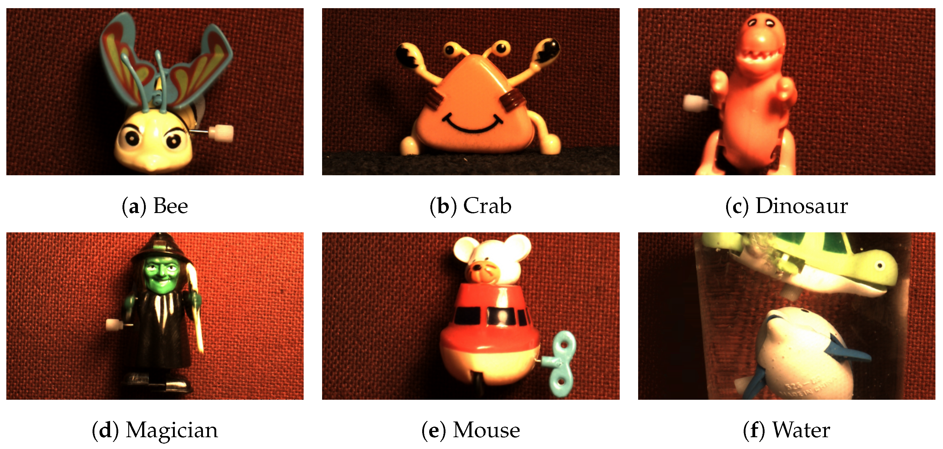
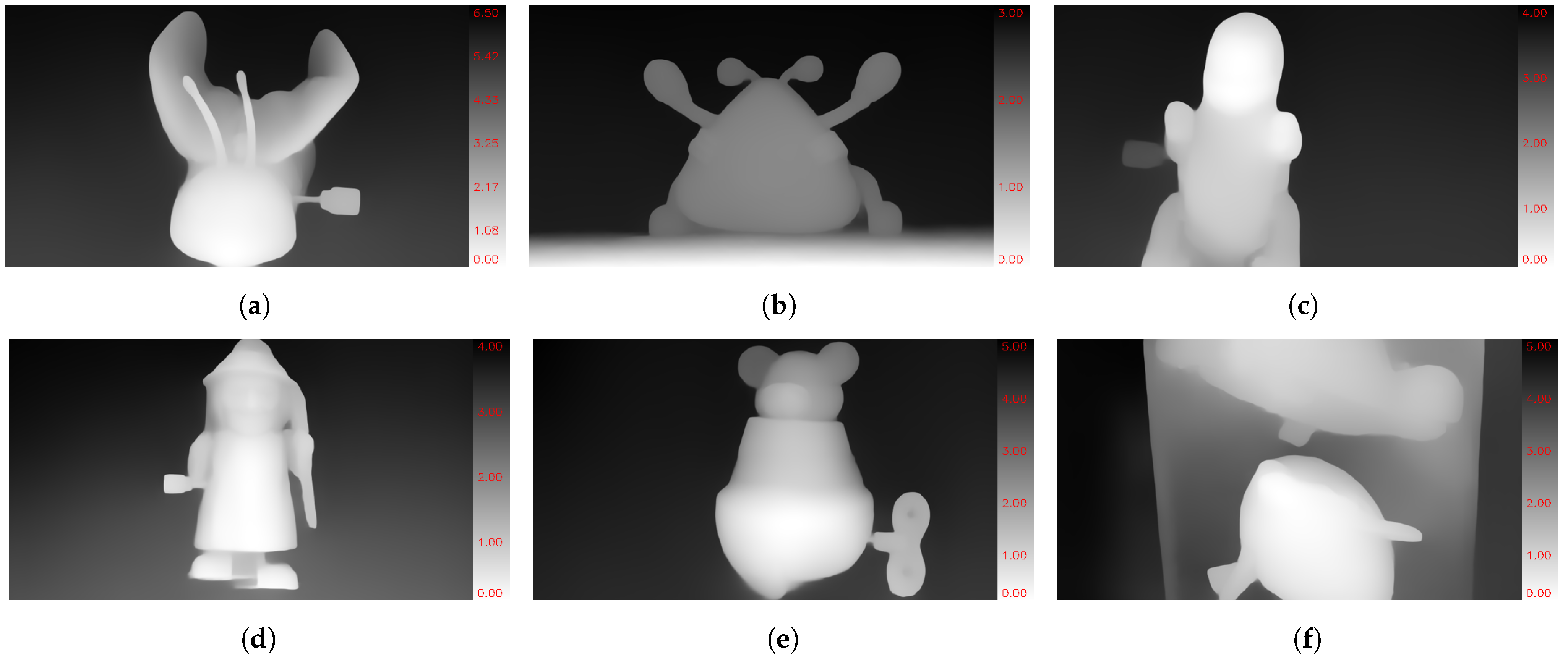
The dataset comprises six distinct sets of video contents and objects. Notably, one of the contents, ‘Water’, is composed of multiple objects rather than a single entity. Furthermore, the ‘Water’ content showcases transparent objects, featuring both a ‘Fish’ and a ‘Turtle’ immersed in a glass of water, thereby presenting transparency for both water and glass. In total, the dataset includes six distinct contents carefully chosen for the light-field dataset, offering diverse characteristics such as object composition complexity, colour intricacy, and motion variety. Figure 1 shows a sample view for each content available in the dataset and Figure 2 depicts their depth map view samples.
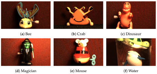
Figure 1.
Raytrix R8 view samples. (a–f) subfigures illustrate the view samples of Bee, Crab, Dinosaur, Magician, Mouse, and Water contents, respectively.
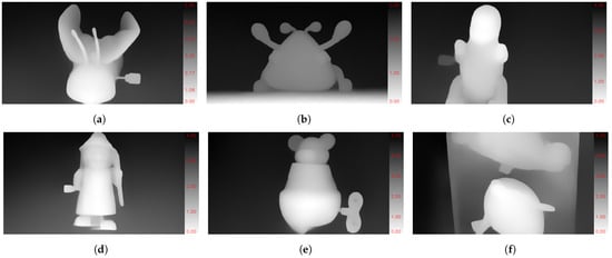
Figure 2.
Raytrix R8 central view depth samples with the scale bar in (cm). (a–f) subfigures illustrate the depth maps of Bee, Crab, Dinosaur, Magician, Mouse, and Water contents, respectively.
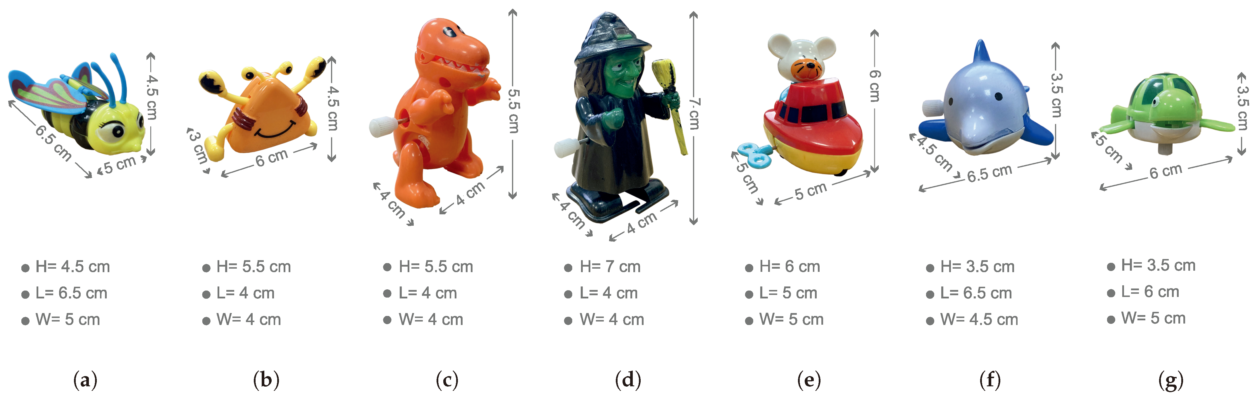
All available models (Bee, Crab, Dinosaur, Magician, Mouse, and Water) in the dataset are wind-up models made of plastic, and come in a variety of colours. Notably, in one specific content, ‘Water’, there are multiple objects, specifically two models of ‘Fish’ and ‘Turtle’. Figure 3 provides a visual representation of all the models used in the dataset, along with their corresponding geometry details.

Figure 3.
The geometry details of each of the used models are as follows: (a) Bee, (b) Crab, (c) Dinosaur, (d) Magician, (e) Mouse, and two models are used for the Water content, which are (f) Fish and (g) Turtle.
4. Content Characterisation Methodologies
The characterisation of the contents is evaluated using various metrics, including motion vector, SI, TI, and CF, which are explained individually below.
4.1. Motion Vector
In this work, unlike in previous similar ones, we did not use a turntable to control the motion of the models in the dataset, which results in variable motion among different models. To evaluate these motion displacements, motion vector algorithms are employed. Specifically, the Lucas–Kanade optical flow algorithm [47] is selected for this purpose. This algorithm operates by detecting object corners and comparing consecutive frames to generate motion vectors. For every two consecutive frames, central views are extracted and converted into HSV color space images. The ‘V’ component of the HSV images is utilised to apply the Lucas–Kanade optical flow equation and determine the available motion vectors. Each motion vector has an initial point () and an end point (). The change in the x-direction () and the change in the y-direction () are calculated as follows:
Next, the magnitude of each motion vector is computed using the Euclidean distance formula [48], which is given by
The set provided in (4) contains all available calculated velocities derived from the motion vectors calculated using the equation above (for each single available pair of frames).
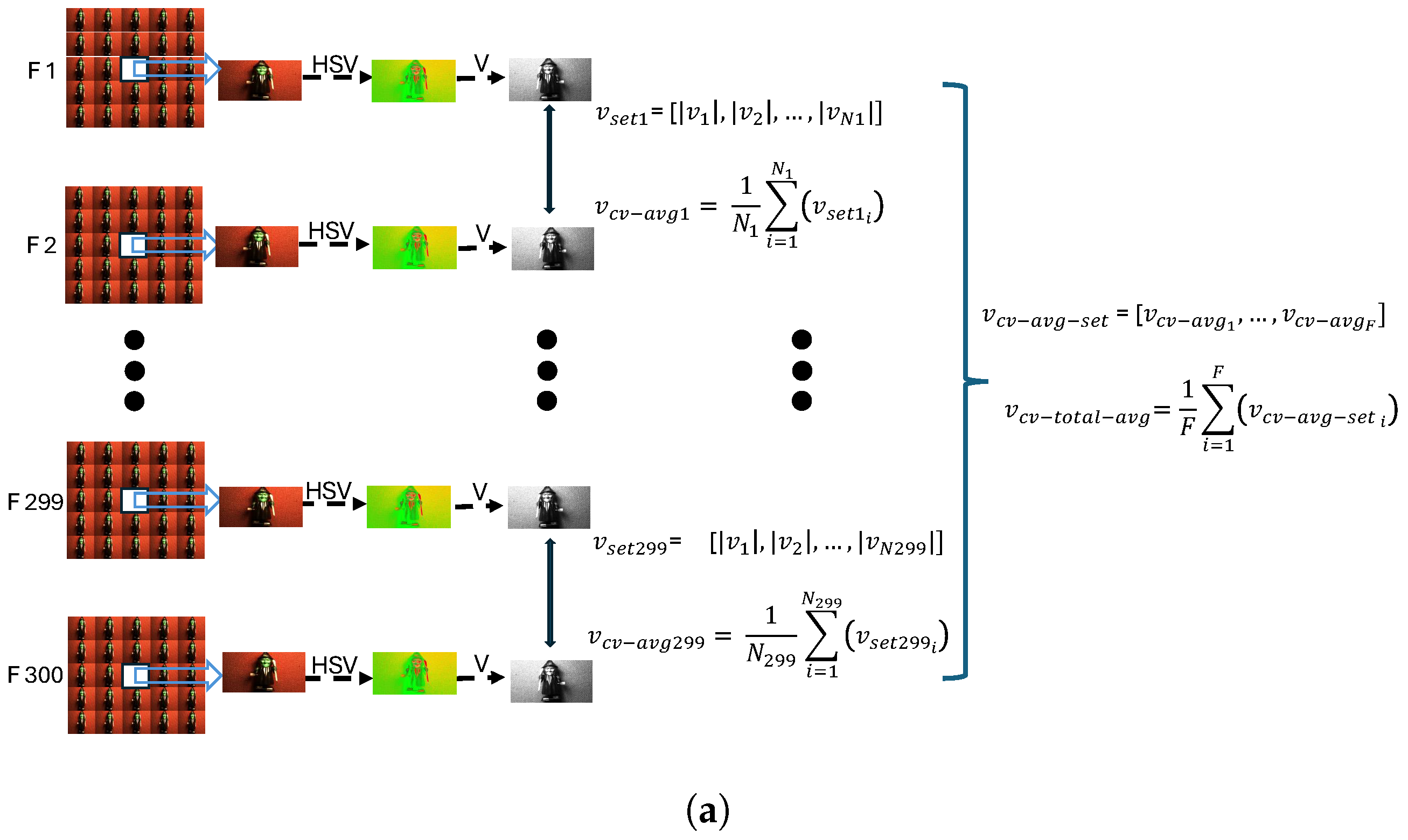
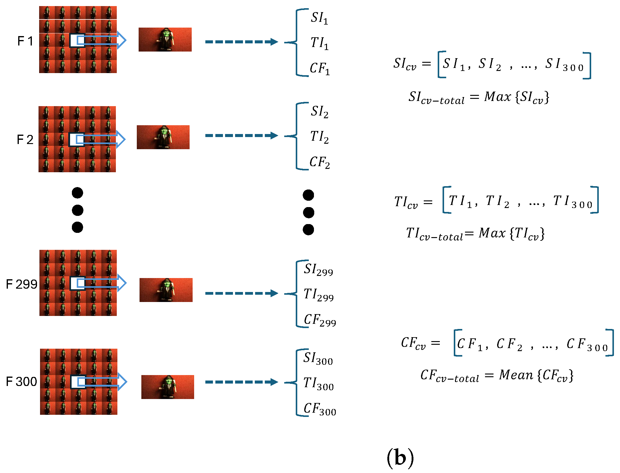
Referring to Figure 4a, each pair of central views from consecutive frames is evaluated to determine the motion vector displacements between them. Consequently, the mentioned N value in Figure 4a varies for each pair of consecutive frames and is denoted as , , …, . To calculate the overall average value of motion displacements, in Equation (7), F is used, representing the total number of frame pairs. For a light-field video consisting of 300 frames, F equals 299 frame pairs. Moreover, the average of (4) is calculated in (5) to yield a single value representing the motion displacement between the two consecutive frames.
where N represents the number of available motion vectors for each pair of consecutive frames, and it can vary for each pair. Here, a ‘frame’ refers to the central view of each grid of views. Additionally, the cv subscript in (5) refers to the ‘central view’ of the 25 quilted views in the light-field frame. By applying Equations (4) and (5) to all available pairs of frames in each video, we obtain the set
where F is the number of consecutive frame pairs in each video, which is equal to 299. To achieve the final motion displacement for each video, the average of (6) is calculated:

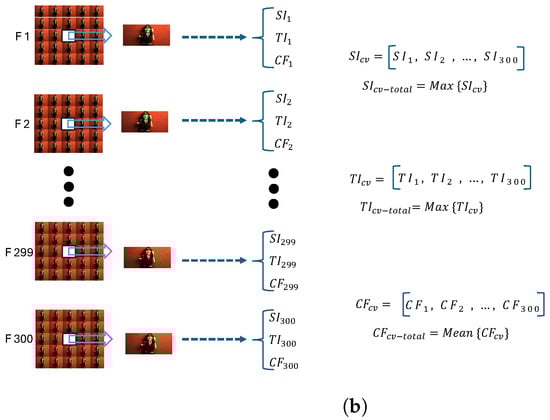
Figure 4.
Content characterisation evaluation flows for (a) motion displacement characterisation flow, and (b) , , and characterisation flow.
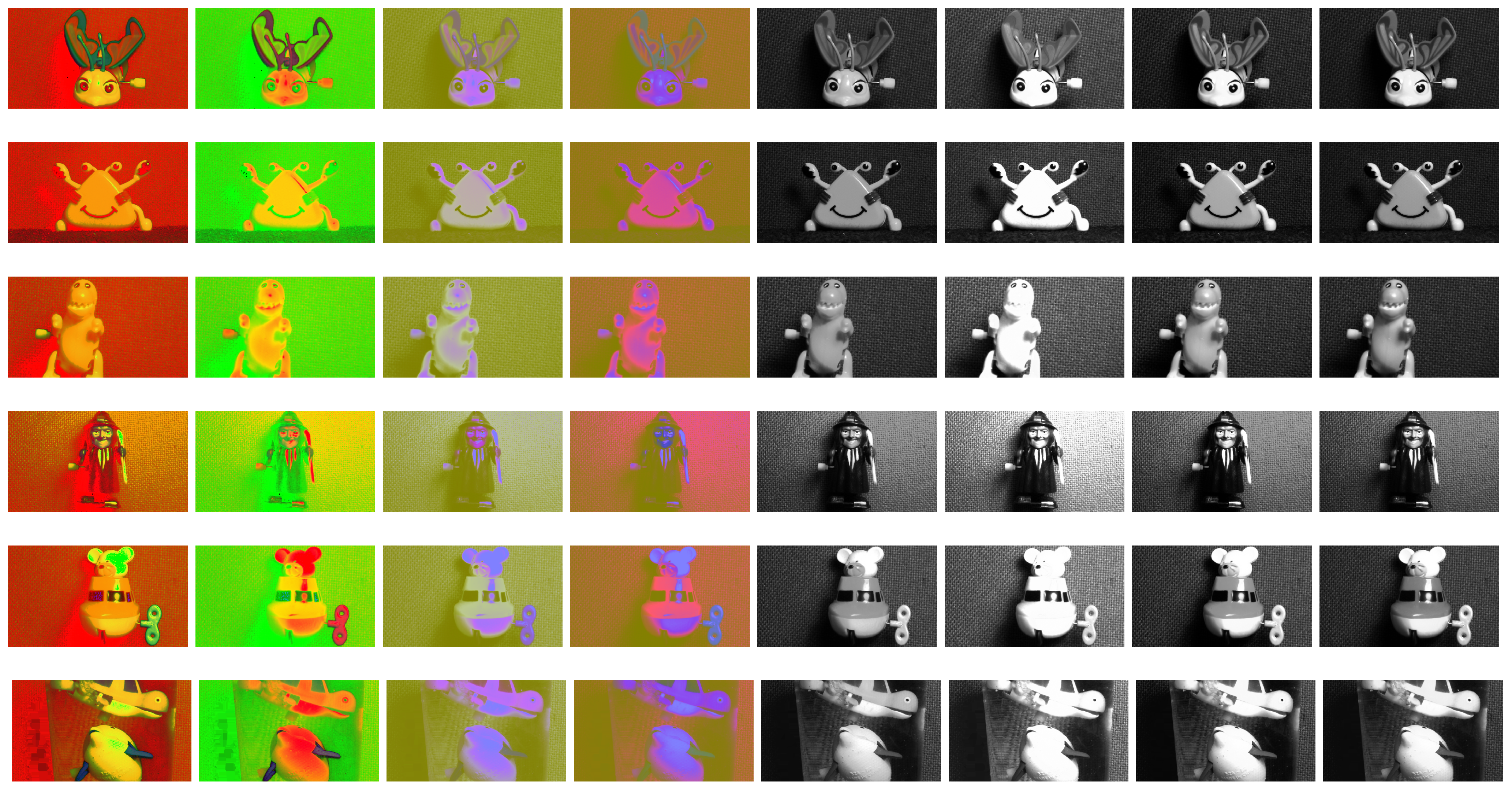
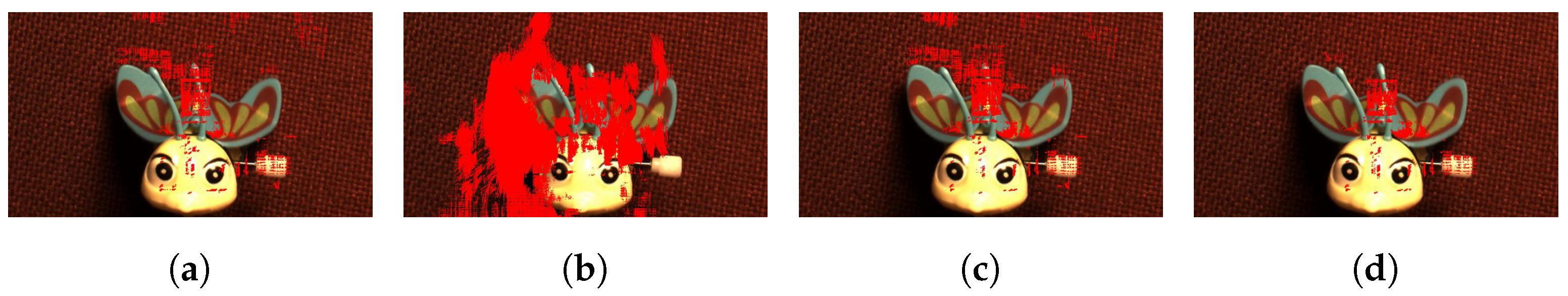
Due to the high motion displacements observed in certain models within the dataset, such as ‘Bee’, accurately determining motion vectors presents a challenge. To address this issue, various colour spaces are applied to the light-field contents of the dataset. For all available light-field video contents in the dataset, different colour spaces, including hue, saturation, luminance (HSL); hue, saturation, value (HSV); Lab*; and YUV (Luminance (Y) and Chrominance (UV)) are utilised [49]. The (L) component in HSL, (V) component in HSV, (L) component in LAB, and (Y) component in YUV are employed to determine the motion vectors, as illustrated in Figure 5. The HSV colour space appears to be the most suitable for calculating the motion vectors, as shown in Figure 6. In the second image displayed, representing the HSV colour space of the ‘Bee’ content, the motion vectors are most accurately detected around the model’s wings. This precision explains why the HSV color space is employed to determine the overall motion displacements across all the light-field video contents in the dataset. Following this, Figure 7 showcases all detected motion vectors when the HSV color space is applied. These vectors are displayed across all pairs of successive frames in the video, encompassing a comprehensive overview of the detected motion vectors for all available models in the dataset. Therefore, to calculate the total motion displacement values in the dataset, the central view is initially converted to an HSV color space image, and then the (V) component in the HSV image is utilised for further calculations. Additionally, for both SI and TI, as depicted in Figure 8a,b, respectively, the (V) component of the HSV image is employed to apply the Sobel filter. Consequently, the term ‘HSV’ is appended for both the vertical and horizontal axes of the figures.

Figure 5.
Each row of images represents one content in the different color spaces HSL, HSV, LAB, and YUV (in order from left to right for the first four sample images) followed by the (L) component for HSL, (V) component for HSV, (L) component for LAB, and (Y) component for YUV (sorted in each row from five to eight). The view samples reported in the six rows are from the contents ‘Bee’, ‘Crab’, ‘Dinosaur’, ‘Magician’, ‘Mouse’, and ‘Water’.
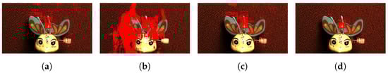
Figure 6.
Detected motion vectors; (a) ‘L’ component in HSL, (b) ‘V’ component in HSV, (c) ‘L’ component in LAB, and (d) ‘Y’ component in YUV.
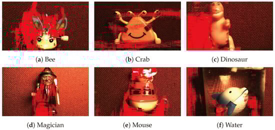
Figure 7.
Overall motion vectors added on a sample view of ‘V’ component in HSV color space. (a–f) subfigures illustrate the motion vectors on Bee, Crab, Dinosaur, Magician, Mouse, and water contents, respectively.
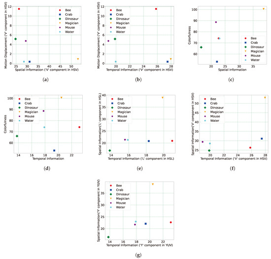
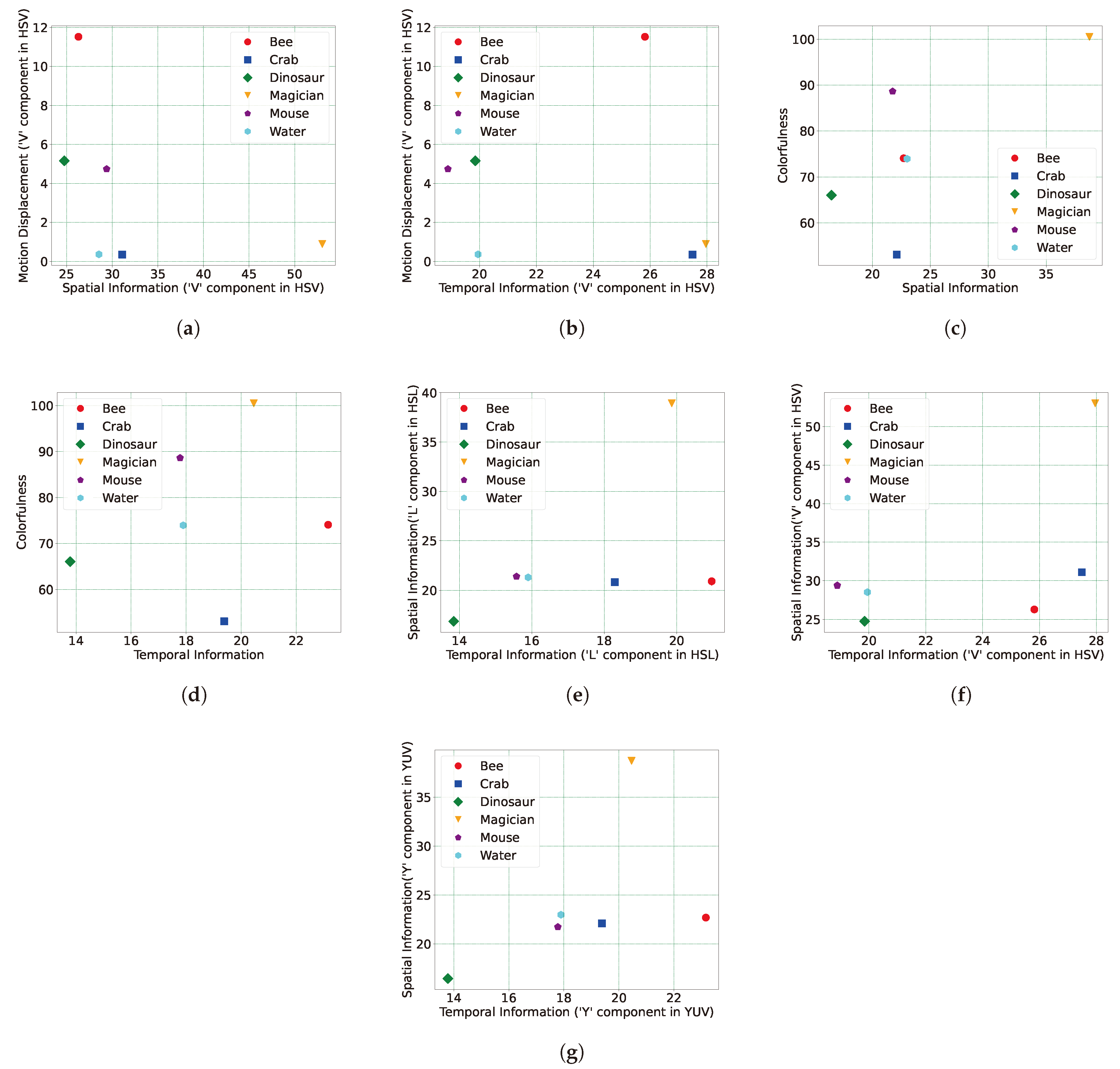
Figure 8.
Content characterisation values in (a,b) present motion displacement values for HSV colour space in the vertical axis versus two of SI and TI, respectively, in the horizontal axis; (c,d) present colourfulness values in the vertical axis and SI and TI, respectively, in the horizontal axis. (e–g) represent SI versus TI values for three colour spaces of HSL, HSV, and YUV, respectively.
4.2. SI, TI, and CF
The central view in each frame of every light-field content is selected as a representative view for measuring Spatial Information (SI), Temporal Information (TI), and colourfulness (CF) values. In total, for 300 frames, this process results in 300 distinctive values. The maximum value among them is then chosen as the final metric value for SI and TI, while the mean value is calculated for the final CF result. For SI, the Sobel filter is applied to the selected central view, and the standard deviation of the Sobel filtered view is then measured. Subsequently, the maximum value among the measured standard deviations over all frames is chosen as the SI value for the light-field content. In all Equations (8)–(18), the subscript “” refers to the central view of the frame, which is located at view position (3,3) in the light-field grid. The mentioned view is initially converted to a grayscale image, following which the Sobel filter is applied in both the vertical and horizontal axes. Equations (8) and (9) illustrate the convolution of the Sobel filter kernel (edge filter) with the central view image of the frame.
where ‘’ represents the intensity of the central view image of the light-field video frame. Then, the magnitude is calculated based on the two components and in both horizontal and vertical axes, respectively:
To find the standard deviation value, the mean value over the pixels is initially calculated:
where H and W in Equation (12) represent the height and width of the central view image, respectively, to determine the number of available pixels. Having the mean value of each Sobel-filtered view in Equation (11), the standard deviation of each central view image is then calculated in Equation (13) [50]:
The maximum standard deviation value over the available central view images in all 300 available frames is picked as a final SI of the light-field video, as calculated in Equation (14):
To compute the TI value of the light-field content, the subtraction of pixel values between each available pair of subsequent views in the light-field video is calculated. The standard deviation is then computed for the resulting values from the mentioned subtraction, and the maximum among all values for all 300 frames is then selected as the final TI value for the light-field content. The corresponding pixels from the central view images in two successive frames are subtracted:
Then, the standard deviation is calculated:
and finally, as is the case for SI, the maximum value over all resulted standard deviation over all available frames is calculated as the final TI value of the light-field video:
To determine the CF characterisation of the available video contents in the dataset, the same central view of each frame is selected to calculate the CF value. Subsequently, the mean of all CF values across all 300 frames is chosen as the final CF of the light-field content. In contrast to SI and TI, for CF, the mean value over all obtained results is calculated as the final CF value for the content. The CF for a single central view () is calculated in Equation (18).
where represents the standard deviation and the mean value; and are found based on the equations below:
Finally, to achieve the total CF value for each video content, the mean overall CF values are measured in Equation (21)
where F is the number of available frames in each video. All the calculation steps for the SI, TI, and CF values are depicted in Figure 4b. This figure shows the three characteristic parameters for each central view of the frames. For SI and TI, the maximum values are selected, while for CF, the mean value is chosen as the final result.
5. Analysis of the Content Characterisation Results
After applying the characterisation metrics for the available light-field contents, this section presents and evaluates the obtained results. The results are divided into two sections: the first section focuses on motion vectors, while the second section encompasses SI, TI, and CF metrics collectively.
5.1. Motion Vectors Results Analysis
The results obtained via the motion vector metric are illustrated in two figures, Figure 8a,b. In both figures, the vertical axis shows the motion displacement values versus the SI and TI, respectively. The motion displacement values are derived using the HSV colour space applied to the dataset contents. Upon analysis, it becomes evident that the motion displacement in the ‘Bee’, ‘Dinosaur’, and ‘Mouse’ video contents is higher than in other contents. For instance, in the case of the ‘Bee’ model, this can be attributed to the rapid motion of the flying wings within the ‘Bee’ content. Furthermore, this result justifies the presence of motion blur effects in these three contents, considering the effect of the 30-frame-rate value of the Raytrix R8 plenoptic camera. Conversely, the lowest motion displacement values belong to the ‘Water’, ‘Crab’, and ‘Magician’ models, respectively.
5.2. SI, TI, and CF Results Analysis
Figure 8c illustrates the comparison between CF (y-axis) and SI (x-axis) and Figure 8d shows the CF values in the vertical axis versus the TI values on the horizontal axis of the plot. Upon examining the results, it is evident that the content labelled ‘Bee’ exhibits the highest TI score among all the presented contents in the dataset, while content ‘Dinosaur’ records the lowest TI score among the video contents. Regarding CF, ‘Magician’ demonstrates the highest score, while the lowest is observed for ‘Crab’. Figure 8e–g present the comparison between SI (y-axis) and TI (x-axis), where three different colour spaces (HSL, HSV, and YUV) are applied on the view samples. This indicates the highest SI score for the content ‘Magician’, aligning with the CF plots. The highest SI value associated with the ‘Magician’ model can be attributed to its texture complexity. As indicated by Equations (8), (9), and (13), the Sobel filter (an edge filter) is initially applied to detect edges in the central view. The standard deviation over the Sobel-filtered view is then calculated as part of the SI measurement process. It is evident that models with greater texture complexity exhibit more edges, leading to higher standard deviation values in the view. Upon comparing the models in the dataset, it becomes apparent that the ‘Magician’ model possesses the highest texture complexity, a conclusion corroborated by the SI measurement. Conversely, the lowest SI score is recorded for ‘Dinosaur’, while, in the case of CF, the lowest score was for the ‘Crab’ content. As mentioned in the introduction section, each content in the dataset possesses its own motion speeds, and these speeds are not controlled by any external instrument to ensure a constant speed for all available objects. Consequently, upon examining the content named ‘Dinosaur’, it becomes evident that its spatial information is limited. This is attributed to the content having the lowest texture complexity.
6. Light-Field Dataset Objective Quality Assessment
This section outlines the procedure for evaluating the quality of the generated light-field plenoptic video contents during their encoding process by various video encoders. The process begins with the encoding of the videos using multiple video encoders, followed by a detailed explanation of quality evaluation using PSNR and SSIM.
6.1. Light-Field Video Encoding Procedure
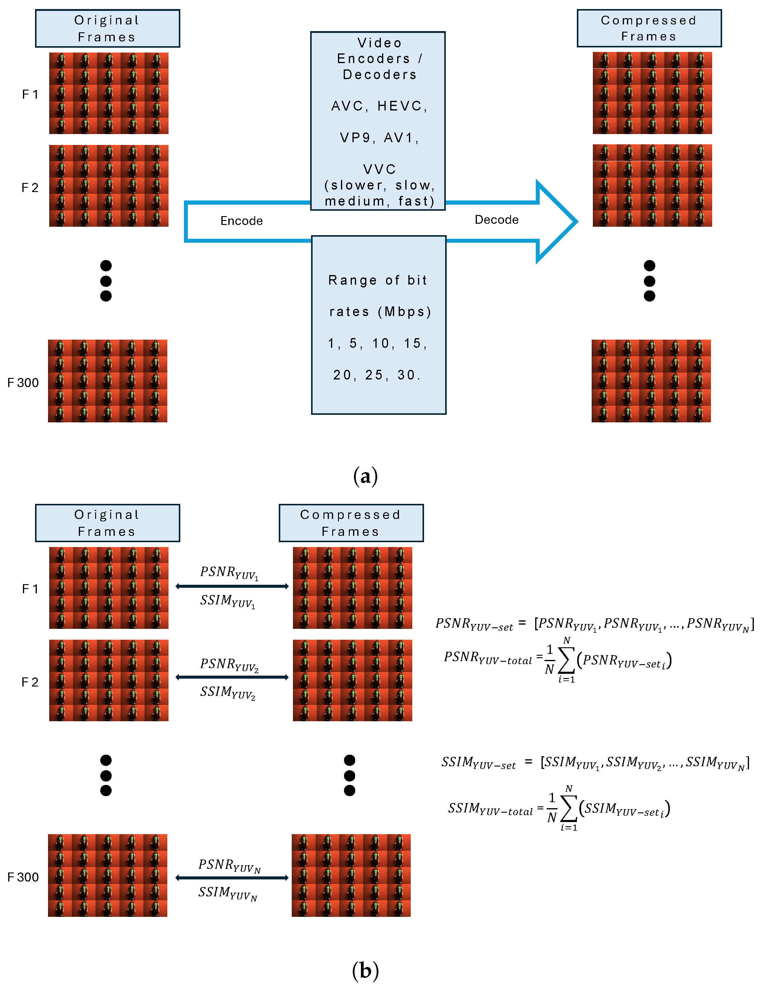
We used various video encoders, namely AVC [6], HEVC [7], VP9 [8], AV1 [9], and VVC (VVenc and VVdec) [10,11], at different bit rate ranges (1, 5, 10, 15, 20, 25, 30) megabits per second initially, followed by decoding on the other side. Specifically for VVenc, four speed settings (fast, medium, slow, and slower) were employed. All contents input during the encoding phase consisted of 25 views with a spatial resolution of pixels for each view, arranged in a quilt with an angular resolution of , which resulted in spatial resolution of pixels for each plenoptic light-field frame.
6.2. PSNR and SSIM Quality Metrics
The primary assessment procedure is outlined in Figure 9, illustrating both the encoding process (Figure 9a) and the comprehensive quality assessment flow incorporating PSNR and SSIM metrics (Figure 9b). the provided decoded light-field video contents from the preceding section were subsequently evaluated in comparison with their original versions to demonstrate objective quality values. Two quality metrics, PSNR [51] and SSIM [52], were selected to objectively assess the quality of the available light-field contents in the dataset. All evaluations for both and were based on the average of the values for YUV components. Initially, the quilted original frames for each individual light-field video content were encoded using the respective mentioned video encoders, each time targeting specific bit-rate values, as mentioned above. Subsequently, the encoded light-field videos were decoded. Each decoded video was then compared frame by frame with the original video. Since each frame was compared, this process yielded 300 distinct values each time for both PSNR and SSIM quality metrics.
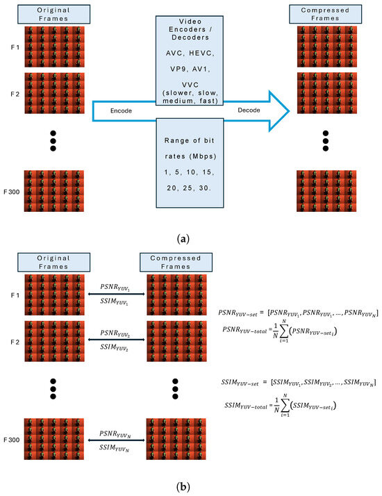
Figure 9.
Quality assessment encompasses two main components: (a) the encode–decode procedure applied to the light-field video contents, and (b) the evaluation of quality metrics such as PSNR and SSIM.
Each member of the sets in (22) and (23) represents the quality metric value for one frame of the decoded videos. Finally, based on (24) and (25), the average of each set of 300 values is calculated as the result of each metric for each video.
Here, N represents the number of available PSNR and SSIM values in the two presented sets of (22) and (23), which, for the dataset, is equal to 300. The two final sets in (26) and (27) provide the total values for each of the PSNR and SSIM quality metrics across all the bitrate values.
Regarding the relationship between PSNR and SSIM, here, we remind the reader that these are related and, for DCT-based compression of reasonable quality, one can be obtained from the other, as highlighted in [53].
6.3. Objective Quality Assessment Discussion
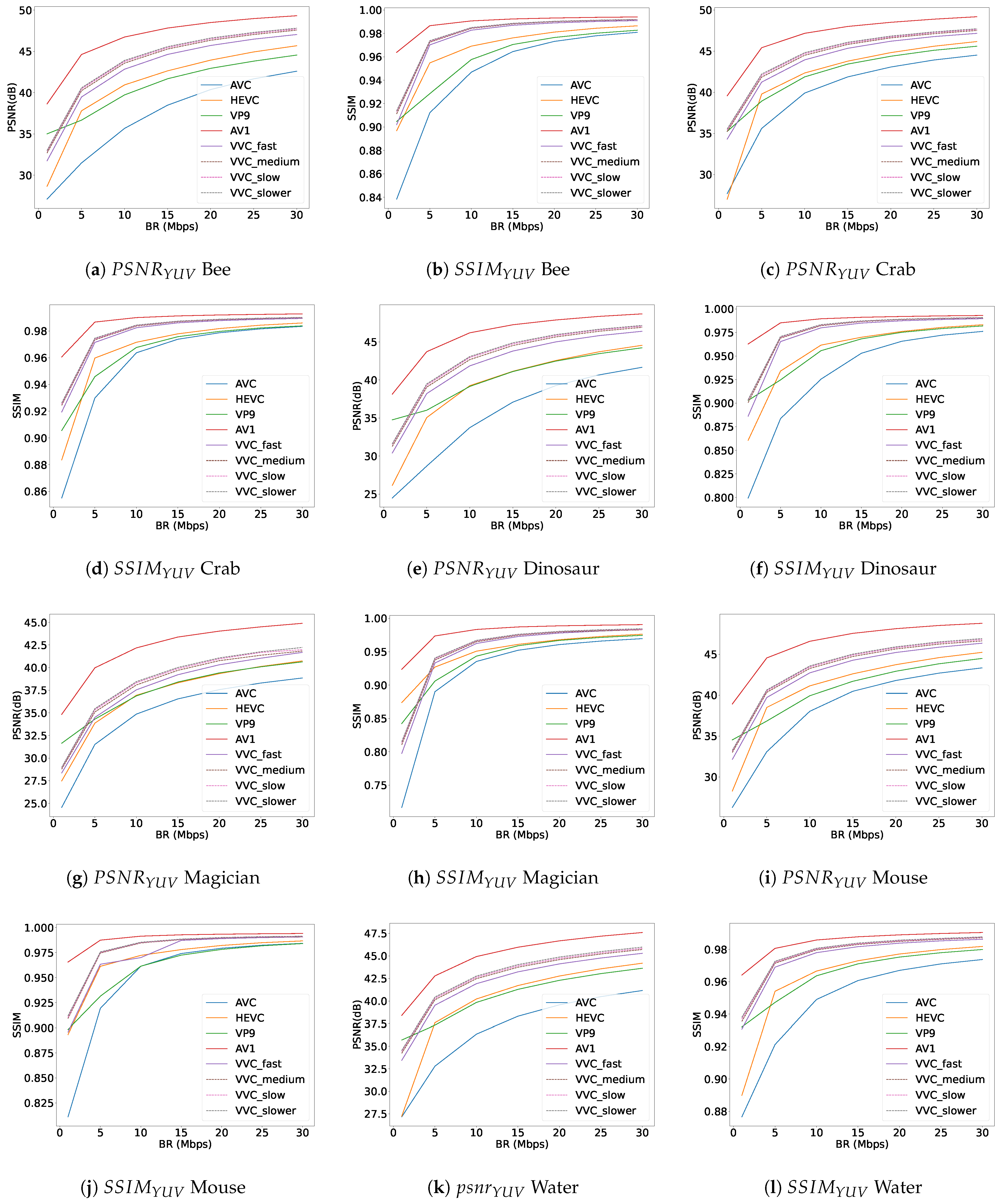
The results for the PSNR and SSIM objective quality metrics are reported in Figure 10, which consists of twelve subplots. Each subplot displays graphs for PSNR and SSIM, representing the quality metrics values for all six available light-field video contents on the vertical axis versus seven different bit-rate (Mbps) values on the horizontal axis across the dataset. A comparison with our previous paper [49], which utilised a light-field dataset from a nonplenoptic camera with a spatial resolution of pixels for each view, reveals interesting observations. In the previous dataset, VP9 outperformed HEVC and occupied a higher position than the HEVC encoder. However, in the current plenoptic light-field video dataset with a frame spatial resolution of pixels, HEVC exhibits better quality in most bit-rate ranges. Additionally, the VVC encoder, across all four different speeds, consistently underperforms compared to the AV1 encoder, indicating a weaker performance than AV1. The diagrams also demonstrate that decreasing the VVC encoder preset speed leads to only marginal improvements, as shown by the dashed lines representing the slow, fast, and faster presets in Figure 10. Furthermore, Table 1, which details several available light-field datasets, includes information on the acquisition camera types and the content types, whether they are light-field video datasets or light-field image datasets. The datasets mentioned in both Table 1 and Table 2 are selected based on whether plenoptic cameras are used for the dataset, if the dataset is a light-field video dataset, or if the light-field dataset contains either characterisation evaluations or quality assessments. Table 2 indicates whether the available light-field contents in each dataset have been evaluated for either objective quality metrics or content characterisation. By reviewing Table 2, it is evident that our dataset, KULFR8, is evaluated for all the mentioned content characterisation and objective quality metrics of PSNR and SSIM. Additionally, there is no similar video plenoptic dataset containing the mentioned evaluations available for comparison with the results obtained in this paper.
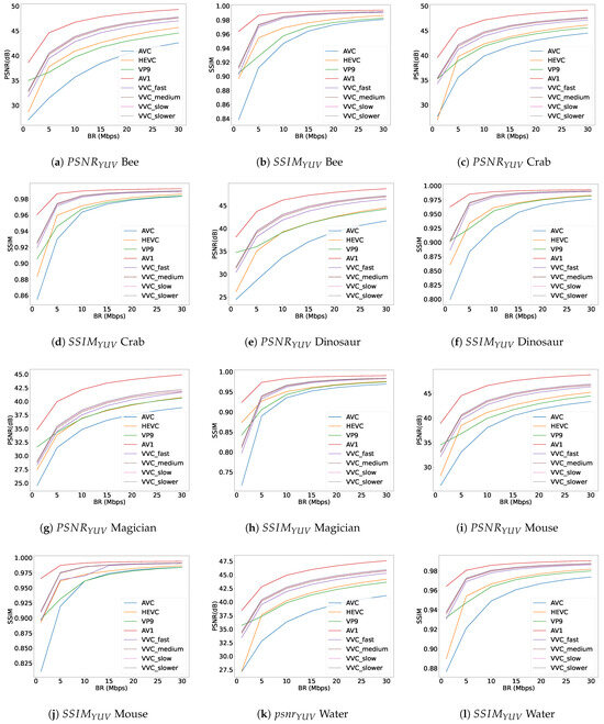
Figure 10.
Quality metric plots and for ‘Bee’, ‘Crab’, ‘Dinosaur’, ‘Magician’, ‘Mouse’, and ‘Water’ light-field video contents.

Table 1.
Summary of datasets and their acquisition parameters.
Table 2.
Summary of datasets and their quality parameters.
7. Conclusions
As an emerging technology, light-field contents should be widely accessible to researchers to support advancements in light-field 3D technology. In this paper, we created a light-field video dataset, KULFR8, which was captured with a plenoptic camera, specifically the Raytrix R8. The dataset comprises six distinct light-field video contents, each containing 300 frames with a duration of ten seconds, captured at a frame rate of 30 fps. For the acquired contents, different characterisation metrics are evaluated, including motion displacements, SI, TI, and CF. The contents were compressed with five different encoders, AVC, HEVC, VP9, AV1, and VVC (in four preset modes), with each encoder producing videos at seven compression ratios; hence, 336 compressed videos are obtained. For these videos, the objective quality metrics PSNR and SSIM were calculated. Given the substantial number of views and frames in this dataset, due to the number of available quilted frames and the number of available views in the dataset, one potential use case is the development of machine learning algorithms for further analysis. In future work, we plan to run subjective tests on the compressed light-field videos in this dataset in order to provide a reliable quality evaluation of the videos in the dataset and to support the development of objective quality assessment metrics based on machine learning, where the machine learning will help to estimate the results of subjective scores. Another interesting future study, as suggested by a reviewer, would be to perform rate-distortion comparisons of light field compression via encoding versus compressed light field sensing [59].
Author Contributions
Conceptualisation, K.J. and M.G.M.; methodology, K.J. and M.G.M.; validation, K.J.; investigation, K.J.; resources, K.J. and M.G.M.; writing—original draft preparation K.J., review and editing M.G.M.; visualisation, K.J.; supervision, M.G.M.; project administration, M.G.M. All authors have read and agreed to the published version of the manuscript.
Funding
This research received no external funding.
Data Availability Statement
The dataset is publicly available via the following link: https://bit.ly/KULF-R8.
Acknowledgments
Kamran Javidi would like to thank Edris Shafiee for his assistance in introducing the light field equipment used in this project.
Conflicts of Interest
The authors declare no conflict of interest.
Abbreviations
The following abbreviations are used in this manuscript:
| AV1 | AOMedia Video 1 |
| AVC | Advanced Video Coding |
| CF | Colourfulness |
| fps | frames per second |
| HEVC | High Efficiency Video Coding |
| HSV | Hue-Saturation-Value |
| HSL | Hue-Saturation-Lightness |
| Mbps | Megabits per second |
| ML | Machine Learning |
| PSNR | Peak Signal-to-Noise Ratio |
| RGB | Red, Green, Blue |
| SI | Spatial Information |
| SR | Super Resolution |
| SSIM | Structural Similarity Index |
| TI | Temporal Information |
| VVC | Versatile Video Coding |
| VP9 | Video Codec 9 |
References
- Wu, G.; Masia, B.; Jarabo, A.; Zhang, Y.; Wang, L.; Dai, Q.; Chai, T.; Liu, Y. Light field image processing: An overview. IEEE J. Sel. Top. Signal Process. 2017, 11, 926–954. [Google Scholar] [CrossRef]
- Levoy, M.; Hanrahan, P. Light field rendering. In Proceedings of the 23rd Annual Conference on Computer Graphics and Interactive Techniques, New Orleans, LA, USA, 4–9 August 1996; pp. 31–42. [Google Scholar]
- Wang, Y.; Wang, L.; Liang, Z.; Yang, J.; Timofte, R.; Guo, Y.; Jin, K.; Wei, Z.; Yang, A.; Guo, S.; et al. NTIRE 2023 challenge on light field image super-resolution: Dataset, methods and results. In Proceedings of the IEEE/CVF Conference on Computer Vision and Pattern Recognition, Vancouver, BC, Canada, 18–22 June 2023; pp. 1320–1335. [Google Scholar]
- Schambach, M.; Heizmann, M. A multispectral light field dataset and framework for light field deep learning. IEEE Access 2020, 8, 193492–193502. [Google Scholar] [CrossRef]
- Jin, J.; Hou, J.; Chen, J.; Kwong, S. Light field spatial super-resolution via deep combinatorial geometry embedding and structural consistency regularization. In Proceedings of the IEEE/CVF Conference on Computer Vision and Pattern Recognition, Seattle, WA, USA, 13–19 June 2020; pp. 2260–2269. [Google Scholar]
- ITU-T Recommendation H.264: Advanced Video Coding for Generic Audiovisual Services. 2003. Available online: https://www.itu.int/rec/T-REC-H.264 (accessed on 20 April 2024).
- ITU-T Recommendation H.265: High Efficiency Video Coding. 2013. Available online: https://www.itu.int/rec/T-REC-H.265 (accessed on 20 April 2024).
- Internet Engineering Task Force (IETF) RFC 7741, WebM Project: VP9 Bitstream Specification. 2016. Available online: https://www.webmproject.org/vp9/ (accessed on 20 April 2024).
- Alliance for Open Media: AV1 Bitstream and Decoding Process Specification. 2021. Available online: https://aomedia.org/av1-features/ (accessed on 20 April 2024).
- Wieckowski, A.; Brandenburg, J.; Hinz, T.; Bartnik, C.; George, V.; Hege, G.; Helmrich, C.; Henkel, A.; Lehmann, C.; Stoffers, C.; et al. VVenC: An Open And Optimized VVC Encoder Implementation. In Proceedings of the IEEE International Conference on Multimedia Expo Workshops (ICMEW), Abu Dhabi, United Arab Emirates, 25–28 October 2020; pp. 1–2. [Google Scholar] [CrossRef]
- Wieckowski, A.; Hege, G.; Bartnik, C.; Lehmann, C.; Stoffers, C.; Bross, B.; Marpe, D. Towards A Live Software Decoder Implementation For The Upcoming Versatile Video Coding (VVC) Codec. In Proceedings of the 2020 IEEE International Conference on Image Processing (ICIP), Abu Dhabi, United Arab Emirates, 25–28 October 2020; pp. 3124–3128. [Google Scholar] [CrossRef]
- Guillo, L.; Jiang, X.; Lafruit, G.; Guillemot, C. Light Field Video Dataset Captured by a R8 Raytrix Camera (with Disparity Maps); Technical Report; International Telecommunication Union (ITU): Geneva, Switzerland, 2018. [Google Scholar]
- Wang, B.; Peng, Q.; Wang, E.; Han, K.; Xiang, W. Region-of-interest compression and view synthesis for light field video streaming. IEEE Access 2019, 7, 41183–41192. [Google Scholar] [CrossRef]
- Shafiee, E.; Martini, M.G. Datasets for the quality assessment of light field imaging: Comparison and future directions. IEEE Access 2023, 11, 15014–15029. [Google Scholar] [CrossRef]
- Wanner, S.; Meister, S.; Goldluecke, B. Datasets and benchmarks for densely sampled 4D light fields. Vision Model. Vis. 2013, 13, 225–226. [Google Scholar]
- Tao, M.W.; Hadap, S.; Malik, J.; Ramamoorthi, R. Depth from combining defocus and correspondence using light-field cameras. In Proceedings of the IEEE International Conference on Computer Vision, Sydney, Australia, 1–8 December 2013; pp. 673–680. [Google Scholar]
- Li, N.; Ye, J.; Ji, Y.; Ling, H.; Yu, J. Saliency detection on light field. In Proceedings of the IEEE Conference on Computer Vision and Pattern Recognition, Columbus, OH, USA, 23–28 June 2014; pp. 2806–2813. [Google Scholar]
- Yoon, Y.; Jeon, H.G.; Yoo, D.; Lee, J.Y.; So Kweon, I. Learning a deep convolutional network for light-field image super-resolution. In Proceedings of the IEEE International Conference on Computer Vision Workshops, Santiago, Chile, 7–13 December 2015; pp. 24–32. [Google Scholar]
- Rerabek, M.; Ebrahimi, T. New light field image dataset. In Proceedings of the 8th International Conference on Quality of Multimedia Experience (QoMEX), Lisbon, Portugal, 6–8 June 2016. [Google Scholar]
- Paudyal, P.; Olsson, R.; Sjöström, M.; Battisti, F.; Carli, M. SMART: A Light Field Image Quality Dataset. In Proceedings of the 7th International Conference on Multimedia Systems, Wörthersee, Austria, 10–13 May 2016; pp. 1–6. [Google Scholar]
- Sabater, N.; Boisson, G.; Vandame, B.; Kerbiriou, P.; Babon, F.; Hog, M.; Gendrot, R.; Langlois, T.; Bureller, O.; Schubert, A.; et al. Dataset and pipeline for multi-view light-field video. In Proceedings of the EEE Conference on Computer Vision and Pattern Recognition Workshops, Honolulu, HI, USA, 21–26 July 2017; pp. 30–40. [Google Scholar]
- Honauer, K.; Johannsen, O.; Kondermann, D.; Goldluecke, B. A dataset and evaluation methodology for depth estimation on 4D light fields. In Computer Vision–ACCV 2016, Proceedings of the 13th Asian Conference on Computer Vision, Taipei, Taiwan, 20–24 November 2016; Revised Selected Papers, Part III 13; Springer: Berlin/Heidelberg, Germany, 2017; pp. 19–34. [Google Scholar]
- Shekhar, S.; Kunz Beigpour, S.; Ziegler, M.; Chwesiuk, M.; Paleń, D.; Myszkowski, K.; Keinert, J.; Mantiuk, R.; Didyk, P. Light-field intrinsic dataset. In Proceedings of the he British Machine Vision Conference 2018 (BMVC), Newcastle, UK, 3–6 September 2018. [Google Scholar]
- de Faria, S.M.; Filipe, J.N.; Pereira, P.M.; Tavora, L.M.; Assuncao, P.A.; Santos, M.O.; Fonseca-Pinto, R.; Santiago, F.; Dominguez, V.; Henrique, M. Light field image dataset of skin lesions. In Proceedings of the 2019 41st Annual International Conference of the IEEE Engineering in Medicine and Biology Society (EMBC), Berlin, Germany, 23–27 July 2019. [Google Scholar]
- Hu, X.; Wang, C.; Pan, Y.; Liu, Y.; Wang, Y.; Liu, Y.; Zhang, L.; Shirmohammadi, S. 4DLFVD: A 4D light field video dataset. In Proceedings of the 12th ACM Multimedia Systems Conference, Chengdu, China, 20–24 October 2021; pp. 287–292. [Google Scholar]
- Sheng, H.; Cong, R.; Yang, D.; Chen, R.; Wang, S.; Cui, Z. UrbanLF: A comprehensive light field dataset for semantic segmentation of urban scenes. IEEE Trans. Circuits Syst. Video Technol. 2022, 32, 7880–7893. [Google Scholar] [CrossRef]
- Wang, T.C.; Zhu, J.Y.; Kalantari, N.K.; Efros, A.A.; Ramamoorthi, R. Light field video capture using a learning-based hybrid imaging system. ACM Trans. Graph. 2017, 36, 1–13. [Google Scholar] [CrossRef]
- Sakamoto, T.; Kodama, K.; Hamamoto, T. A study on efficient compression of multi-focus images for dense light-field reconstruction. In Proceedings of the 2012 Visual Communications and Image Processing, IEEE, San Diego, CA, USA, 27–30 November 2012; pp. 1–6. [Google Scholar]
- Marwah, K.; Wetzstein, G.; Bando, Y.; Raskar, R. Compressive light field photography using overcomplete dictionaries and optimized projections. ACM Trans. Graph. 2013, 32, 1–12. [Google Scholar] [CrossRef]
- Tambe, S.; Veeraraghavan, A.; Agrawal, A. Towards motion aware light field video for dynamic scenes. In Proceedings of the IEEE International Conference on Computer Vision, Sydney, Australia, 1–8 December 2013; pp. 1009–1016. [Google Scholar]
- Perra, C. On the coding of plenoptic raw images. In Proceedings of the 2014 22nd Telecommunications Forum Telfor (TELFOR), IEEE, Belgrade, Serbia, 25–27 November 2014; pp. 850–853. [Google Scholar]
- Choudhury, C.; Tarun, Y.; Rajwade, A.; Chaudhuri, S. Low bit-rate compression of video and light-field data using coded snapshots and learned dictionaries. In Proceedings of the 2015 IEEE 17th International Workshop on Multimedia Signal Processing (MMSP), Xiamen, China, 6–11 June 2015; pp. 1–6. [Google Scholar]
- Thomaz, L.A.; Santos, J.M.; Astola, P.; de Faria, S.M.; Assunçao, P.A.; de Carvalho, M.B.; da Silva, E.A.; Pagliari, C.L.; Tabus, I.; Pereira, M.P.; et al. Visually lossless compression of light fields. In Proceedings of the European Light Field Imaging Workshop, Borovets, Bulgaria, 4–6 June 2019. [Google Scholar]
- Hedayati, E.; Havens, T.C.; Bos, J.P. Light field compression by residual CNN-assisted JPEG. In Proceedings of the 2021 International Joint Conference on Neural Networks (IJCNN), Virtual Conference, 18–22 July 2021; pp. 1–9. [Google Scholar]
- Shidanshidi, H.; Safaei, F.; Li, W. Estimation of signal distortion using effective sampling density for light field-based free viewpoint video. IEEE Trans. Multimed. 2015, 17, 1677–1693. [Google Scholar] [CrossRef]
- Singh, M.; Rameshan, R.M. Learning-based practical light field image compression using a disparity-aware model. In Proceedings of the 2021 Picture Coding Symposium (PCS), Virtual Conference, 29 June–2 July 2021; pp. 1–5. [Google Scholar]
- Avramelos, V.; De Praeter, J.; Van Wallendael, G.; Lambert, P. Light field image compression using versatile video coding. In Proceedings of the 2019 IEEE 9th International Conference on Consumer Electronics (ICCE-Berlin), Berlin, Germany, 8–11 September 2019; pp. 70–75. [Google Scholar]
- JPEG Pleno Light Field Datasets. Available online: https://plenodb.jpeg.org/lf/pleno_lf (accessed on 14 May 2024).
- Amirpour, H.; Pinheiro, A.; Pereira, M.; Lopes, F.J.; Ghanbari, M. Efficient light field image compression with enhanced random access. ACM Trans. Multimed. Comput. Commun. Appl. 2022, 18, 1–18. [Google Scholar] [CrossRef]
- Barina, D.; Solony, M.; Chlubna, T.; Dlabaja, D.; Klima, O.; Zemcik, P. Comparison of light field compression methods. Multimed. Tools Appl. 2022, 81, 2517–2528. [Google Scholar] [CrossRef]
- IEEE P3333.1.4-WG; IEEE P3333.1.4 Recommended Practice on the Quality Assessment of Light Field Imaging. IEEE Standards Association: Piscataway, NJ, USA, 2022.
- Kara, P.A.; Tamboli, R.R.; Shafiee, E.; Martini, M.G.; Simon, A.; Guindy, M. Beyond perceptual thresholds and personal preference: Towards novel research questions and methodologies of quality of experience studies on light field visualization. Electronics 2022, 11, 953. [Google Scholar] [CrossRef]
- Raytrix Light Field Camera. Available online: http://www.raytrix.de/ (accessed on 20 April 2024).
- Raytrix Light Field Camera Sensor Details. Available online: https://raytrix.de/products/ (accessed on 20 May 2024).
- Raytrix Light Field Camera Field of View Details. Available online: https://raytrix.de/examples/ (accessed on 20 May 2024).
- Raytrix Light Field Camera Depth Resolution. Available online: https://raytrix.de/technology-2/ (accessed on 20 May 2024).
- Lucas, B.D.; Kanade, T. An iterative image registration technique with an application to stereo vision. In Proceedings of the IJCAI’81: 7th International Joint Conference on Artificial Intelligence, Vancouver, BC, Canada, 24–28 August 1981; Volume 2. [Google Scholar]
- Danielsson, P.E. Euclidean distance mapping. Comput. Graph. Image Process. 1980, 14, 227–248. [Google Scholar] [CrossRef]
- Javidi, K.; Martini, M.G.; Kara, P.A. KULF-TT53: A Display-Specific Turntable-Based Light Field Dataset for Subjective Quality Assessment. Electronics 2023, 12, 4868. [Google Scholar] [CrossRef]
- Zhang, R.; Regunathan, S.L.; Rose, K. Video coding with optimal inter/intra-mode switching for packet loss resilience. IEEE J. Sel. Areas Commun. 2000, 18, 966–976. [Google Scholar] [CrossRef]
- ITU-T Study Group 16. Working Practices Using Objective Metrics for Evaluation of Video Coding Efficiency Experiments; Technical Report; International Telecommunication Union: Geneva, Switzerland, 2020. [Google Scholar]
- Wang, Z.; Simoncelli, E.P.; Bovik, A.C. Multiscale structural similarity for image quality assessment. In Proceedings of the The Thrity-Seventh Asilomar Conference on Signals, Systems & Computers, Pacific Grove, CA, USA, 9–12 November 2003; IEEE: Piscataway, NJ, USA; Volume 2, pp. 1398–1402. [Google Scholar]
- Martini, M. A simple relationship between SSIM and PSNR for DCT-based compressed images and video: SSIM as content-aware PSNR. In Proceedings of the 2023 IEEE 25th International Workshop on Multimedia Signal Processing (MMSP), Poitiers, France, 27–29 September 2023; pp. 1–5. [Google Scholar]
- Viola, I.; Ebrahimi, T. VALID: Visual quality assessment for light field images dataset. In Proceedings of the 2018 Tenth International Conference on Quality of Multimedia Experience (QoMEX), Cagliari, Italy, 29 May–1 June 2018; pp. 1–3. [Google Scholar]
- Zizien, A.; Fliegel, K. LFDD: Light field image dataset for performance evaluation of objective quality metrics. In Proceedings of the Applications of Digital Image Processing XLIII, SPIE, Online, 24 August–4 September 2020; Volume 11510, pp. 671–683. [Google Scholar]
- Kiran Adhikarla, V.; Vinkler, M.; Sumin, D.; Mantiuk, R.K.; Myszkowski, K.; Seidel, H.P.; Didyk, P. Towards a quality metric for dense light fields. In Proceedings of the IEEE Conference on Computer Vision and Pattern Recognition, Honolulu, HI, USA, 21–26 July 2017; pp. 58–67. [Google Scholar]
- Ahmad, W.; Palmieri, L.; Koch, R.; Sjöström, M. Matching light field datasets from plenoptic cameras 1.0 and 2.0. In Proceedings of the 2018-3DTV-Conference: The True Vision-Capture, Transmission and Display of 3D Video (3DTV-CON), Helsinki, Finland, 3–5 June 2018; pp. 1–4. [Google Scholar]
- Shi, L.; Zhao, S.; Zhou, W.; Chen, Z. Perceptual evaluation of light field image. In Proceedings of the 2018 25th IEEE International Conference on Image Processing (ICIP), Athens, Greece, 7–10 October 2018; pp. 41–45. [Google Scholar]
- Feng, X.; Ma, Y.; Gao, L. Compact light field photography towards versatile three-dimensional vision. Nat. Commun. 2022, 13, 3333. [Google Scholar] [CrossRef] [PubMed]

Disclaimer/Publisher’s Note: The statements, opinions and data contained in all publications are solely those of the individual author(s) and contributor(s) and not of MDPI and/or the editor(s). MDPI and/or the editor(s) disclaim responsibility for any injury to people or property resulting from any ideas, methods, instructions or products referred to in the content. |
© 2024 by the authors. Licensee MDPI, Basel, Switzerland. This article is an open access article distributed under the terms and conditions of the Creative Commons Attribution (CC BY) license (https://creativecommons.org/licenses/by/4.0/).