Abstract
In data-driven bearing fault diagnosis, sufficient fault data are fundamental for algorithm training and validation. However, only very few fault measurements can be provided in most industrial applications, bringing the dynamics model to produce bearing response under defects. This paper built a Modelica model for the whole bearing test rig, including the test bearing, driving motor and hydraulic loading system. First, a five degree-of-freedom (5-DoF) model was proposed for the test bearing to identify the normal bearing dynamics. Next, a fault model was applied to characterize the defect position, defect size, defect shape and multiple defects. The virtual bearing test bench was first developed with OpenModelica and then called in Python with OMPython. For validation of the positive effect of the dynamics model in the direct transfer learning for bearing fault diagnosis, the simulation data from the Modelica model and experimental data from the Case Western Reserve University were fed separately or jointly to train a Convolution Neural Network (CNN). Then the well-trained CNN was transferred directly to achieve the fault diagnosis under the test set consisting of experiment data. Additionally, 157 features were extracted from both time-domain and frequency-domain and fed into CNN as input, and then four different validation cases were designed. The results confirmed the positive effect of simulation data in the CNN transfer learning, especially when the simulation data were added as auxiliary to experimental data, and improved CNN classification accuracy. Furthermore, it indicated that the simulation data from the bearing dynamics model could play a part in the actual experimental measurement when the collected data were insufficient.
1. Introduction
Bearing fault diagnosis and prognosis can effectively prevent rotating machines from most failures and therefore have much significance. In recent years, data-driven methods have gained increasing attention in this field, and many good results have been achieved. Among the different kinds of data-driven methods, Convolution Neural Network (CNN) is the most commonly used due to its powerful ability in deep feature extraction and complex nonlinear mapping. CNN was first introduced to realize bearing fault diagnosis by O. Janssens in 2016 [1]. Thereafter, many improvements and variants have been proposed to strengthen the CNN’s performance, such as 1D-CNN, 2D-CNN, multiscale CNN and adaptive CNN [2,3,4,5]. Though satisfying results have been obtained in the extensive research mentioned above, the premise to guarantee such results for data-driven methods is sufficient data for algorithm training. However, in practice, limited rather than massive data are typical, which has become a significant barrier of data-driven PHM (Prognostics and Health Management) being applied in industrial settings. Data augmentation and generation have been adopted to address this problem. Oversampling was first proposed for data generation, and the main idea is to generate more samples by direct replication for such labels that had very few ones [6,7]. Although this method is simple and efficient to implement, causes overfitting easily since no new information is incorporated. As another perspective method for data generation, Generative Adversarial Network (GAN) has already been used for new sample generation in fault diagnosis, generating new samples similar to the actual measurement with random noise input. Both W. Zhang and S. Shao employed GAN to create more vibration data and to expand the available imbalanced dataset, with results confirming that the diagnosis accuracy could be improved once the imbalanced data was augmented by GAN [8,9].
This previous research has proven effective in sample generation for small or imbalanced datasets. Still, most of these methods are data-driven and generate new samples merely based on the given existing measurements or random noise, ignoring the physics mechanism behind data. This brings bearing dynamics model as an alternative to produce bearing response under given normal and defect conditions. To date, the methods for bearing dynamics and vibration response simulation can be classified into two categories, namely, mechanism-based models and signal-based models. Cui et al. proposed a 5-DoF model to describe bearing’s dynamic behavior [10]. Moreover, a defect model was built to address defect position, defect shape and defect size [11]. In terms of bearing response simulation based on signal analysis, the first model was proposed by McFadden in 1983 to identify the amplitude spectrum of bearing with a single defect on the inner race [12]. In 2000, slight random variations were incorporated into the impulse responses to resemble actual vibration signals generated by bearing faults [13]. After that, Cong et al. put forward a new fault signal model for bearing with the combination of decaying oscillation fault signal model and rotor dynamic response influence [14]. In a real test bench, dynamics from driving and loading systems also affect the test bearing response. Nevertheless, to our exhausted knowledge, nearly all published papers on bearing fault modeling only focus on the bearing without considering the dynamics from driving motor and loading actuator, also very limited work has been reported on bearing modeling in Modelica, which defines the goal to build a whole bearing test bench in this study [15]. In this paper, a virtual bearing test bench is developed in OpenModelica, including test bearing, connecting shaft, hydraulic loading and force controller, driving motor and speed controller. The test bearing dynamics model elaborates under normal conditions and various defect scenarios. After validation, the virtual test bench is used to generate simulation samples. Afterward, the generated samples are fed into CNN for network training. Finally, the well-trained CNN is transferred directly to achieve fault diagnosis on pure experiment data collected from the Case Western Reserve University bearing test rig.
The main innovation of this paper includes: (1) A general platform for bearing dynamics simulation and CNN-based fault diagnosis is developed based on OpenModelica and Python. The calling method and interface are presented, giving a new and efficient solution for studying the data-driven fault diagnosis with open source languages. (2) The simulation data from the dynamics model was used for CNN training. In addition, the positive effect on the CNN’s transfer learning performance from the generated simulation data was studied and analyzed with four designed validation cases.
This paper’s remaining part is structured as follows: Section 2 introduces the modeling theory of bearing dynamics with defects. Section 3 details the implementation process of the bearing dynamics model in OpenModelica and the calling interface in Python with OMPython. After that, the feature extraction and fault diagnosis based on CNN are presented in Section 4. Section 5 describes the direct transfer learning of CNN from the simulation model to the test bench when involved in bearing fault diagnosis and analyzes the positive effect from simulation data. Finally, Section 6 concludes the whole paper.
2. Dynamics Modeling of Bearing with Defects
The ball bearing comprises the outer ring, inner ring, cage and rolling elements. A standard bearing achieves dynamic balance in a stable operating condition, while a series of impulses will be generated once there is a defect between the contact surfaces. A 5-DoF dynamics model and a defect model will be introduced in the following.
2.1. The Nonlinear 5-DoF Model
This model describes the nonlinear dynamic behavior of bearing, as shown in Figure 1. In the 5-DoF model, 4 DoF represents the horizontal and vertical directions of inner and outer rings, and 1 DoF stands for the vertical direction of the resonator, which is modeled as the spring-mass system [10].
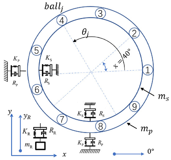
Figure 1.
The 5-DoF model of bearing [10].
Based on Newton’s second law, the bearing dynamic equilibrium equations can be formulated as Equation (1) [10].
and are contact force at x and y axis, respectively, is external load. The meanings and values of other variables can be found in [15]. According to Hertzian contact theory, the contact force between rolling element and raceways can be given by:
with j from 1 to , which represents the number of rolling elements. stands for the ball’s stiffness, denotes deformation. The deformation of the jth ball, , is determined by the displacement between the inner and outer races, the angular position and the total clearance c caused by the oil film and assembly clearance, as:
The angular position of the jth ball can be calculated by Equation (4).
where is initial cage angular position and is cage angular frequency, which can be further obtained from shaft frequency like Equation (5).
where and are the ball diameter and pitch diameter, respectively.
Usually, there is inevitable sliding for bearings in real applications when a ball rolls on the raceways. The sliding direction depends on where the ball is located; when the ball enters the load zone, the angular speed of the ball center is faster than that of the cage; otherwise, the ball would slide backward. Consequently, with sliding considered, the angular position of each ball can be modified by Equation (6) [10].
There are two constants and a sign function in Equation (6). is a parameter defining the mutation percentage of average contact frequency, which is normally between 0.01 and 0.02 rad. is a random number with uniform distribution with the range of , and the sign function is expressed as:
Considering should be nonnegative in physics, its final value is determined by:
2.2. Bearing Defect Model
When bearing has defects either on races or balls, an additional deformation, , will be released when the ball moves over the defect zone. Thus, with defect considered, deformation of the jth ball can be further identified as:
Once bearing deformation under defect is obtained, it can be substituted into Equations (9) and (10). The nonlinear contact force can be calculated and further substituted into Equation (1) for the fault-bearing response. changes with defect position, defect shape and the number of defects. Due to space limitation, only the modeling of defect position will be presented in this paper, the modeling of defect size, defect shape, and multiple defects can be found in the original conference paper [15].
Before defect modeling, four basic geometrical parameters are chosen to feature the defect, as demonstrated in Figure 2, the defect width B, the defect depth , the defect initial angle and the defect span angle . Take a defect on the outer ring as an example, the relation between and B is expressed as:
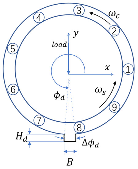
Figure 2.
Size definition of defect on the outer ring [15].
Suppose the local defect depth is , the additional deformation generates only when a ball falls into the defect zone within and , then the deformation released by defect on raceway is given by:
The defect location on the outer ring or inner ring changes with different rules. For the outer ring, the defect is fixed at the defect initial angle . However, for the inner ring, the defect location changes with time when the inner ring rotates. Thus, in Equation (13) can be further modeled as follows.
Different from rings, when a defect happens on a rolling element, the defect spins with ball speed and its position can be obtained like:
hereby the ball speed can be calculated from shaft speed as follows,
The defect on balls contacts the inner and outer ring periodically. Besides, the curvature radii of inner and outer rings are different. Therefore, the same defect span angle produces different angular widths. The angular widths of defect on the outer ring and inner ring, and , can be calculated by Equations (17) and (18).
with and as the diameters of outer ring and inner ring, respectively.
Obviously, the curvature radius determines the depth when ball enters into the raceway, and the curvature radii of ball , inner ring and outer ring can be obtained, respectively, by Equations (19)–(21) [16].
During one revolution of the ball, defect contacts the inner ring and outer ring in succession, with an angular distance of . So, can be given by Equation (22) [16].
Deformation released by fault only appears on the fault ball (kth ball). As a result, the contact deformation with ball defect is given by:
Besides the test bearing, the virtual bearing test bench also consists of a driving module and a loading module. The loading module guarantees that test bearing works under defined external load, and the driving module is responsible for speed profile definition. In this research, the driving module is modeled by a DC motor and a shaft, while the loading module is modeled by an electro-hydraulic servo system. More details about the modeling of these two modules are introduced in [15].
3. Model Implementation in Modelica and Model Calling in Python
To build a general and efficient platform for bearing dynamics simulation and data-driven fault diagnosis, two open-source languages, OpenModelica and Python, are selected in this paper. The former is an object-oriented non-causal multi-domain modeling language, and the latter is a popular open language for data analysis, especially for machine learning and deep learning. In this section, the model structure, virtual bearing test bench, and implementation process in Modelica will be introduced. The interface between Modelica and Python will also be explained shortly.
3.1. Overview of the Virtual Bearing Test Bench in Modelica
First, based on the mathematical models derived above, a model library is created for the virtual bearing test bench in OpenModelica-v1.16.0. As shown in Figure 3a, three main modules like TestBearings, DrivingSystem and LoadingSystem, are packaged and can be used as plug-in components. Each component contains many modules and is also sub-packaged with corresponding names. For example, the TestBearings package provides three instance models: Healthy, RaceDefect and BallDefect, and a Components sub-package containing a DoF model and another sub-package named DefectModel. These models can be constructed into any configuration as required. All components, sub-packages, and models can be used separately or in combination to meet user demand. In Figure 3b, the detailed layout of the whole virtual bearing test bench is presented, which consists of modules from the library in Figure 3a, like the driving module, load module and test bearing module. Specifically, the driving module includes a motor, a shaft and a PID controller, which provides a stable shaft speed for the test bearing. The loading module comprises an electro-hydraulic servo system and a PID controller, which outputs a steady radial load for the test bearing. The shaft speed (‘omega’) and radial load (‘load’) are regulated by two corresponding PID controllers. As to the test bearing module, as illustrated in Figure 3c, it has two inputs, like shaft speed and external load, and one output, acceleration ().
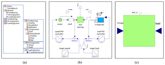
Figure 3.
Bearing test bench in Modelica: (a) Component and module library; (b) Layout of virtual bearing test bench; (c) Interface of test bearing [15].
3.2. Procedure of Simulation with Virtual Bearing Test Bench in Modelica
Figure 4 illustrates the procedure of simulation with the virtual bearing test bench in Modelica. Firstly, users need to choose one working sub-module from the healthy, raceway defect and ball defect bearing sub-modules for the test bearing and configure the simulation setups such as simulation time, interval and output format. Subsequently, all virtual bearing test bench parameters should be configured, including geometrical and material parameters, defect properties and operating parameters. The last step is to run the simulation and obtain the results.
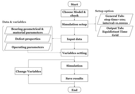
Figure 4.
Simulation flowchart with virtual bearing test bench in Modelica [15].
3.3. Calling Modelica Model in Python with OMPython
As mentioned above, the virtual bearing test bench was developed in Modelica. However, Modelica has relatively limited support for advanced signal analysis and data-driven intelligent algorithm development [17]. On the contrary, due to being empowered by numerous third-party modules and extensive support libraries, especially on machine learning and deep learning, Python is very suitable for developing the data-driven fault diagnosis algorithm. Therefore, to explore a possible framework to combine these two open-source languages, a GUI has been developed in Python to run the Modelica model of the ‘virtual bearing test bench’ in this study. This procedure is realized with Python 3.7.9, OMPython and PyQt5, where OMPython is a Python interface to communicate with OpenModelica via CORBA or ZeroMQ. In this paper, ZeroMQ is used. Furthermore, to operate the OpenModelica model in Python through OMPython, the user can firstly import Python class ‘ModelicaSystem’ from the ‘OMPython’ package. Then the OpenModelica model can be loaded and built as an object in Python. Additionally, users can operate the model in Python via class ‘ModelicaSystem’ and other standard get methods, traditional set methods, simulation methods. Finally, the simulation results can also be acquired and processed as demand.
3.4. Bearing Dynamics Model Validation
Based on the developed GUI and Modelica model, users can simulate the bearing dynamics response under any reasonably defined bearing specification, working condition and defect scenario. Based on our experience, when the simulation duration and stepsize are set as 10 s and 0.001, respectively, the simulation can be finished within 2 min. Figure 5 shows the simulation results of standard bearing and defect bearing, including the inner face fault, outer race fault and ball fault. The acceleration envelope shape under different fault positions agrees well with the previously published results [18]. The time interval between the adjacent fault peaks is consistent with the theoretical fault characteristic frequency, which confirms the effectiveness of the virtual bearing test bench in bearing dynamics simulation. More detailed validation and analysis of the virtual bearing test bench can be found in [15].
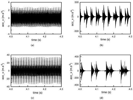
Figure 5.
Simulation results with Modelica model. (a) Normal bearing, (b) Inner race fault, (c) Outer race fault, (d) Ball fault.
4. Bearing Fault Diagnosis Based on CNN
4.1. Cnn Structure and Hyperparameters
LeNet-5 is one of the most frequently used CNN structures. It consists of two sets of convolutional and pooling layers, one flattening layer, two fully-connected layers and one softmax classifier. In this research, it is slightly modified for bearing fault classification. The modified structure is sketched in Figure 6.
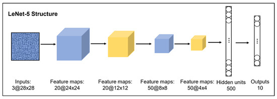
Figure 6.
Structure of LetNet-5 [19].
The hyperparameters of CNN are determined by Particle Swarm Optimization (PSO). The optimized hyperparameters are summarized in Table 1 [19].

Table 1.
Hyperparameters of CNN.
4.2. Feature Extraction from Time and Frequency Domains
Although CNN has a strong ability to extract deep features from data, many researchers still prefer to process the input before it is fed into CNN. When a bearing starts to degrade, the time-domain acceleration response will gradually present non-stationary and non-Gaussian dynamics. Therefore, 13 indexes in total are selected from the time-domain in this work and are presented in Table 2, with kurtosis and skewness characterizing non-Gaussian dynamics, impulse factor, crest factor, standard deviation and shape factor identifying non-stationary characteristics. Similarly, when a defect occurs on the bearing, in the frequency domain, peaks will appear at the corresponding component’s fault characteristic frequencies (FCFs). For example, a bearing with an outer ring fault will produce peaks at the ball pass frequency of the outer race (BPFO) and its harmonics at the frequency spectrum. The same is true for the inner race fault and ball fault, corresponding to the ball pass frequency of the inner race (BPFI) and the ball spin frequency (BSF), respectively. These FCFs contain much information of bearing health condition and therefore are taken to extract the frequency-domain features. Additionally, the fault characteristic frequencies can be affected by many factors, like the shaft speed fluctuation, variant contact angles, external load and sliding movement from rolling elements. Therefore, bias often exists between theoretical and actual BPFs (BPFO, BPFI, BSF). Moreover, some harmonics of BPFs influenced by modulation of other vibrations may not be detected [20]. Thus, to ensure to include the FCFs into frequency-domain features, eight amplitude values around the theoretical FCFs are selected for each order, and FCFs from the 1st to 6th orders are considered. This brings 48 amplitude values for each FCFs (eight values for each order from the first to sixth). This paper considers 3 FCFs, namely BPFI, BPFO and BSF. Hence, 144 frequency-domain features are extracted in total and summarized in Table 3 [19].
Table 2.
Features from time-domain.
Table 3.
Features from frequency-domain.
4.3. Experimental Set Up and Data Preprocessing
The bearing test data used in this paper come from Case Western Reserve University Bearing Data Center. The test stand shown in Figure 7 comprises a two-hp motor, a torque transducer/encoder, a dynamometer, control electronics and test bearings that support the motor shaft. Accelerometers attached to the housing with magnetic bases are used to collect vibration data. Driving end fault data with a sampling frequency of 12 kHz are used in this paper. There are three failure types (ball fault, inner race fault and outer race fault). Aside from standard bearing, each failure type has three different fault diameters (0.007 inches, 0.014 inches and 0.021 inches). In this study, the data from 0.014 to 0.021 inches are addressed separately. Under each defect size, the sample size of the training/test set and labeling method is the same, as shown in Table 4.
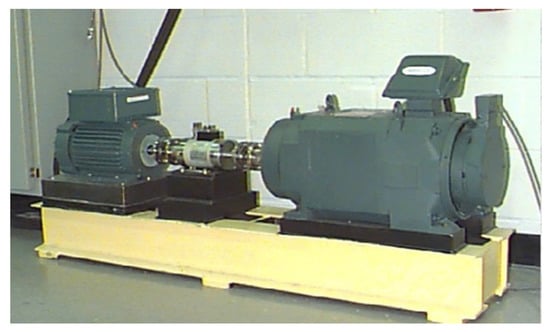
Figure 7.
Experimental setup.
Table 4.
Sample size and labels for training set and test set.
5. Direct Transfer Learning from Simulation Model to Bearing Test Bench
5.1. Procedure Overview of Direct Transfer Learning
As analyzed in the introduction section, sufficient training data are the precondition for data-driven fault diagnosis. Moreover, the training and test sets should belong to the same domain. Otherwise, the accuracy cannot be guaranteed even when the network is trained with enough data from the domain different from the target one. Transfer learning is proposed to solve the network performance reduction when involved across domains. Lei et al. summarized the reported transfer learning methods into four categories [21], like feature-based [22,23], GAN-based [24,25], instance-based [26], and parameter-based [27]. In these published researches, the domain-invariant feature extraction and space alignment should be addressed, either by maximum mean discrepancy constraints or network training or parameter fine-tuning, which is complex and not feasible in industry applications. Essentially, there are two main steps in CNN-based fault diagnosis: feature extraction and feature-label mapping identification. Though the simulation and experiment data come from two different domains, the inevitable differences may arise between them due to the modeling error and some unavailable geometry parameters or parameter identification errors. Nevertheless, there are still some shared features like fault characteristic frequency. Therefore, this research explores whether it is possible to train the CNN with simulation data and part experiment data and then transfer the well-trained CNN to realize the fault diagnosis for a real test bench. Figure 8 demonstrates the procedure of direct transfer learning from the virtual bearing test bench to the Case Western Reserve University bearing test bench.
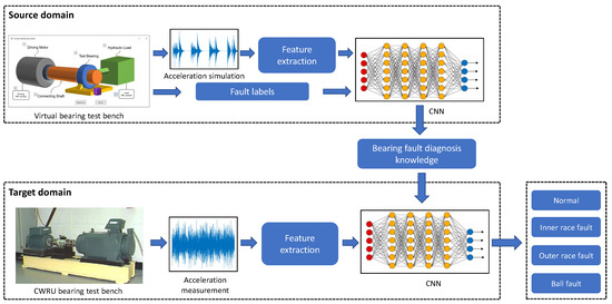
Figure 8.
Process overview of direct transfer learning from dynamics model to test bench.
5.2. Validation Case Design
Four validation cases are designed to thoroughly study and compare the effect of simulation data on the CNN performance when the CNN trained with simulation data is directly transferred to realize fault diagnosis on experiment data. As shown in Table 5, for these four cases, the test set is the same and made up of 1000 sets of experimental data, while the training set is different. In Case A, the training set is pure experiment data, while in Case B, it is pure simulation data. In these two cases, the number of samples in the training set will increase gradually. Case C consists of a fixed number of simulation samples and an increasing number of experiment samples, and Case D is the opposite. These four different cases will be adopted to validate the CNN’s transfer learning ability, namely the training sets from four cases will be used to train the CNN at first. Then the well-trained CNN will be directly transferred to resolve the fault diagnosis on the test set without further training or fine-tuning. Additionally, these designed cases will be validated on cases of 0.014 inches and 0.021 inches separately for complete study and comparison.
Table 5.
Data composition of four validation cases.
5.3. Results of Direct Transfer Learning on Fault Diagnosis
5.3.1. Case A
In the case of A, an increasing number of experimental bearing data is used to train the CNN and then tested under the fixed test set. Here, we must mention that the classification accuracy, i.e., the y axis in figures, refers to the average accuracy of 20 experiment times under the test set. For example, in Figure 9, the ‘25e’ in the x-axis means the CNN is trained with 25 sets of experimental data, and others are in the same manner. As can be seen from Figure 9a,b, the CNN classification accuracy increases with the number of experimental data. Moreover, with the increasing experiment data being fed to train CNN, the CNN classification accuracy rises sharply at first and then slowly. It can be explained as follows: at first, more training data means more information, and more information promotes the CNN to extract more hidden features and enhance the classification accuracy. However, when the training data increase further, most information from the samples is repeated, and only very little new information will be brought in.
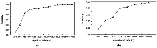
Figure 9.
Fault classification under case A. (a) 0.021 inches, (b) 0.014 inches.
5.3.2. Case B
In the case of B, an increasing number of simulation data is used to train the CNN, and random noise with the same size is also used for CNN training as the contrast. The results are presented in Figure 10, where the ‘25s’ in the x-axis means the CNN is trained with 25 sets of simulation data, and ‘25n’ means the CNN is trained with 25 sets of random noise. As shown in Figure 10, when only simulation data are used as the training data, the CNN classification accuracy is relatively low either for the fault size of 0.021 inches (a) or 0.014 inches (b), but it is still much better than using the random noise. This demonstrates that the simulation data from the bearing dynamics model contains some bearing fault information that the random noise does not have and then contributes to the CNN’s fault diagnosis performance. However, we can find that the classification accuracy does not increase when using more simulation data to train the CNN with further analysis. In Figure 10a, the accuracy rises when the training data increases from 25 sets to 50 sets, and then it even reduces a little bit; In Figure 10b, with increasing simulation data added to the training set, the accuracy increases at first and then fluctuates around the accuracy peak value. Under both two fault sizes, the CNN reaches the accuracy peak values much faster than the CNN trained with experimental data in Figure 9a,b. This is because the bearing fault information in the simulation data are not as abundant as that in experimental data. Moreover, the experimental data also contain process and measurement noise that the dynamics model does not address. Therefore, we can find that only using simulation data as the training data is not feasible with the above results. Thus, employing the simulation data as auxiliary of experiment data to train CNN will be explored and compared in the following cases.
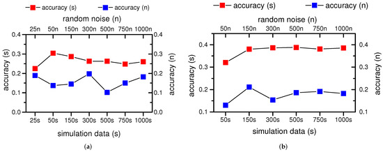
Figure 10.
Fault classification under case B. (a) 0.021 inches, (b) 0.014 inches.
5.3.3. Case C
In the case of C, a different fixed number (50 sets, 150 sets, 500 sets) of simulation data are used as auxiliary data and added to an increasing number of experiment data to train the CNN. The results are illustrated in Figure 11, with the legend ‘cwru’ representing that the CNN was trained with pure experiment data (like case A). The ‘cwru+500s’ refers to the CNN was trained with an increasing number of experiment data (‘cwru’) and fixed 500 sets of simulation data (‘s’), ‘cwru+150s’ and ‘cwru+50s’ are denoted in the same way. The ‘25e+s’ in the x-axis means the CNN is trained with 25 sets of experimental bearing data and a certain fixed number (50 sets, 150 sets, or 500 sets) of simulation data. As Figure 11a shows, no matter 50 sets, 150 sets or 500 sets of simulation data are added as auxiliary data to train the CNN, and the CNN classification accuracy increases much faster than that trained with only experiment data. Besides, when the sample size of experiment data is small, the accuracy improvement is more pronounced. That is to say, regarding the bearing fault diagnosis with CNN, simulation data can provide some supplementary information to speed up the process, especially when the provided experiment training data is limited. Additionally, CNN works even better when the number of simulation data and experiment data in the mixed dataset is similar. The same conclusion can be drawn from the defect size of 0.014 inches in Figure 11b.
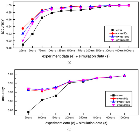
Figure 11.
Fault classification under case C. (a) 0.021 inches, (b) 0.014 inches.
5.3.4. Case D
In contrast to case C, in the case of D, the sample size of experiment data is fixed at certain values (25 sets, 50 sets, 75 sets) and then added to an increasing number of simulation data to train the CNN. Figure 12 gives the results. The legend ‘s+25e’ refers to the CNN trained with 25 sets of experimental data and increasing simulation data. At the same time, the ‘25e’ means the CNN trained with only 25 sets of experiment data (like case A). The other legends are denoted in the same way. As can be seen from Figure 12, when simulation data are added to the experiment data, the CNN classification accuracy is always higher than that from the CNN only trained with experiment data, no matter whether it is 25 sets, 50 sets or 75 sets. These results verify that simulation data as the auxiliary experiment data can improve CNN’s fault classification accuracy. However, the accuracy does not increase as the sample size of simulation data grows, which can be explained as the bearing fault information in the simulation data is relatively repetitive. In short, an appropriate number of simulation data can partly supplement the bearing fault information when experiment data is insufficient. When simulation data are far more than experiment data, it may mislead the classification. That is to say, using simulation data as the auxiliary of experiment data is a more feasible way. With results in Figure 12a,b, the same conclusion can be reached.
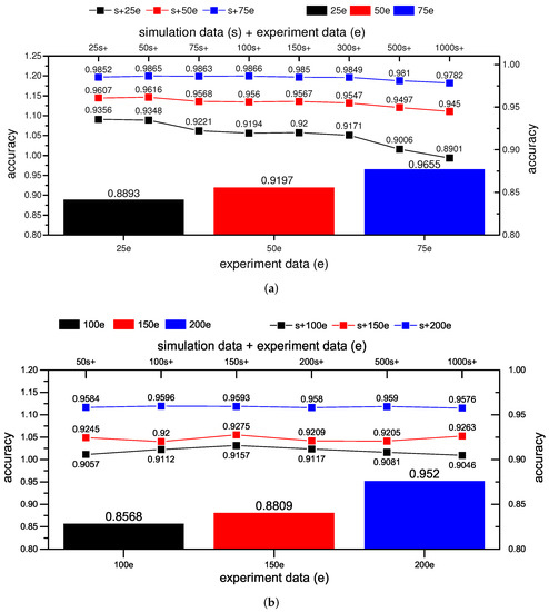
Figure 12.
Fault classification under case D. (a) 0.021 inches, (b) 0.014 inches.
6. Conclusions
Data-driven methods have been intensively used in bearing fault diagnosis, and many satisfying results have been reported. However, nearly all data-driven approaches highly rely on massive data for training. In practice, it is often the case that only limited fault data can be collected, which hinders the application of data-driven fault diagnosis in the industry. This paper developed a virtual bearing test bench in OpenModelica and then used it to generate simulation data for CNN training. The target is to explore whether simulation data from the physics model positively affects CNN fault diagnosis when the well-trained CNN is transferred directly to experimental data. The work can be summarized as follows:
- A virtual bearing test bench has been developed in OpenModelica, with test bearing, driving motor, hydraulic loading and connecting shaft considered. As to the test bearing, besides normal dynamics modeling with the 5-DoF model, the modeling of fault position, shape and size, multiple faults are also addressed.
- The OpenModelica-based virtual bearing test bench is called in Python environment with OMPython and a developed GUI, which serves as a general study platform for data-driven bearing fault diagnosis.
- The simulation data generated from the dynamics model are used to train CNN after feature extraction. The trained-CNN is transferred directly to achieve fault diagnosis under the experimental dataset. Four different validation cases are designed to confirm the simulation data’s positive effect in the CNN’s direct transfer learning for bearing fault diagnosis.
Based on case validation results, we can safely conclude that, compared with random noise, simulation data from the dynamics model have a positive effect in raising CNN’s performance in fault diagnosis. Specifically, using simulation data as auxiliary of experimental data to train CNN is a more feasible way to improve the CNN’s fault classification accuracy. Besides, CNN works even better when the numbers of simulation and experimental data in a mixed dataset are similar.
As to the outlook for further research, improvement in the bearing dynamics model will be the focus, like considering the transient contact angles in modeling. Furthermore, the application of simulation data in more transfer learning scenarios, like domain-invariant feature-based transfer learning, will be explored and compared.
Author Contributions
Conceptualization, D.R. and C.G.; methodology, D.R.; software, Y.C., Z.L. and D.R.; validation, Y.C. and Z.L.; formal analysis, D.R. and Y.C.; investigation, D.R.; resources, D.R.; data curation, D.R. and Y.C.; writing—original draft preparation, D.R. and J.Y.; writing—review and editing, C.G. and J.Y.; visualization, D.R. and J.Y.; supervision, C.G.; project administration, C.G.; funding acquisition, D.R. All authors have read and agreed to the published version of the manuscript.
Funding
This research was funded by CSC (China Scholarship Council) scholarship (201806250024) and Zhejiang Lab’s International Talent Fund for Young Professionals (ZJ2020XT002).
Data Availability Statement
Data supporting the findings of this study are available from the corresponding author upon request.
Acknowledgments
Acknowledgment is made for the bearing dataset published by CWRU.
Conflicts of Interest
The authors declare no conflict of interest.
Abbreviations
The following abbreviations are used in this manuscript:
| PHM | Prognostics and Health Management |
| CNN | Convolutional Neural Networks |
| GAN | Generative Adversarial Network |
| DoF | Degree of Freedom |
| PSO | Particle Swarm Optimization |
| BPFO | Ball Passing Frequency on Outer race |
| BPFI | Ball Passing Frequency on Inner race |
| BSF | Ball Spin Frequency |
| CWRU | Case Western Reserve University |
| GUI | Graphical User Interface |
References
- Janssens, O.; Slavkovikj, V.; Vervisch, B.; Stockman, K.; Loccufier, M.; Verstockt, S.; Van de Walle, R.; Van Hoecke, S. Convolutional neural network based fault detection for rotating machinery. J. Sound Vib. 2016, 377, 331–345. [Google Scholar] [CrossRef]
- Eren, L.; Ince, T.; Kiranyaz, S. A generic intelligent bearing fault diagnosis system using compact adaptive 1D CNN classifier. J. Signal Process. Syst. 2019, 91, 179–189. [Google Scholar] [CrossRef]
- Zhang, W.; Peng, G.; Li, C. Bearings Fault Diagnosis Based on Convolutional Neural Networks with 2-D Representation of Vibration Signals as Input. MATEC Web of Conferences. EDP Sci. 2017, 95, 13001. Available online: https://www.matec-conferences.org/articles/matecconf/abs/2017/09/matecconf_icmme2017_13001/matecconf_icmme2017_13001.html (accessed on 29 January 2022).
- Guo, X.; Chen, L.; Shen, C. Hierarchical adaptive deep convolution neural network and its application to bearing fault diagnosis. Measurement 2016, 93, 490–502. [Google Scholar] [CrossRef]
- Wang, D.; Guo, Q.; Song, Y.; Gao, S.; Li, Y. Application of multiscale learning neural network based on CNN in bearing fault diagnosis. J. Signal Process. Syst. 2019, 91, 1205–1217. [Google Scholar] [CrossRef]
- Cordón, I.; García, S.; Fernández, A.; Herrera, F. Imbalance: Oversampling algorithms for imbalanced classification in R. Knowl.-Based Syst. 2018, 161, 329–341. [Google Scholar] [CrossRef]
- Ren, S.; Zhu, W.; Liao, B.; Li, Z.; Wang, P.; Li, K.; Chen, M.; Li, Z. Selection-based resampling ensemble algorithm for nonstationary imbalanced stream data learning. Knowl.-Based Syst. 2019, 163, 705–722. [Google Scholar] [CrossRef]
- Shao, S.; Wang, P.; Yan, R. Generative adversarial networks for data augmentation in machine fault diagnosis. Comput. Ind. 2019, 106, 85–93. [Google Scholar] [CrossRef]
- Zhang, W.; Li, X.; Jia, X.D.; Ma, H.; Luo, Z.; Li, X. Machinery fault diagnosis with imbalanced data using deep generative adversarial networks. Measurement 2020, 152, 107377. [Google Scholar] [CrossRef]
- Cui, L.; Chen, X.; Chen, S. Dynamics modeling and analysis of local fault of rolling element bearing. Adv. Mech. Eng. 2015, 7, 262351. [Google Scholar] [CrossRef] [Green Version]
- Liu, J.; Shao, Y.; Lim, T.C. Vibration analysis of ball bearings with a localized defect applying piecewise response function. Mech. Mach. Theory 2012, 56, 156–169. [Google Scholar] [CrossRef]
- McFadden, P.; Smith, J. The vibration produced by multiple point defects in a rolling element bearing. J. Sound Vib. 1985, 98, 263–273. [Google Scholar] [CrossRef]
- Ho, D.; Randall, R. Optimisation of bearing diagnostic techniques using simulated and actual bearing fault signals. Mech. Syst. Signal Process. 2000, 14, 763–788. [Google Scholar] [CrossRef]
- Cong, F.; Chen, J.; Dong, G.; Pecht, M. Vibration model of rolling element bearings in a rotor-bearing system for fault diagnosis. J. Sound Vib. 2013, 332, 2081–2097. [Google Scholar] [CrossRef]
- Ruan, D.; Li, Z.; Gühmann, C. Modeling of A Bearing Test Bench and Analysis of Defect Bearing Dynamics in Modelica. In Proceedings of the 14th International Modelica Conference, Linköping, Sweden, 20–24 September 2021; Sjölund, M., Buffoni, L., Pop, A., Ochel, L., Eds.; Number 181 in Linköping Electronic Conference Proceedings. Modelica Association and Linköping University Electronic Press: Linköping, Sweden, 2021; pp. 373–382. [Google Scholar] [CrossRef]
- Mishra, C.; Samantaray, A.; Chakraborty, G. Ball bearing defect models: A study of simulated and experimental fault signatures. J. Sound Vib. 2017, 400, 86–112. [Google Scholar] [CrossRef]
- Lie, B.; Bajrachary, S.; Mengist, A.; Buffoni, L.; Kumar, A.; Sjölund, M.; Asghar, A.; Pop, A.; Fritzson, P. API for accessing OpenModelica models from Python. In Proceedings of the 9th EUROSIM Congress on Modelling and Simulation, Oulu, Finland, 12–16 September 2016; pp. 707–714. [Google Scholar]
- Randall, R.B.; Antoni, J. Rolling element bearing diagnostics—A tutorial. Mech. Syst. Signal Process. 2011, 25, 485–520. [Google Scholar] [CrossRef]
- Ruan, D.; Zhang, F.; Gühmann, C. Exploration and Effect Analysis of Improvement in Convolution Neural Network for Bearing Fault Diagnosis. In Proceedings of the 2021 IEEE International Conference on Prognostics and Health Management (ICPHM), Detroit, MI, USA, 7–9 June 2021; pp. 1–8. [Google Scholar]
- Saruhan, H.; Saridemir, S.; Qicek, A.; Uygur, I. Vibration analysis of rolling element bearings defects. J. Appl. Res. Technol. 2014, 12, 384–395. [Google Scholar] [CrossRef]
- Lei, Y.; Yang, B.; Jiang, X.; Jia, F.; Li, N.; Nandi, A.K. Applications of machine learning to machine fault diagnosis: A review and roadmap. Mech. Syst. Signal Process. 2020, 138, 106587. [Google Scholar] [CrossRef]
- Chen, C.; Li, Z.; Yang, J.; Liang, B. A cross domain feature extraction method based on transfer component analysis for rolling bearing fault diagnosis. In Proceedings of the 2017 29th Chinese Control and Decision Conference (CCDC), Chongqing, China, 28–30 May 2017; pp. 5622–5626. [Google Scholar]
- Tong, Z.; Li, W.; Zhang, B.; Jiang, F.; Zhou, G. Bearing fault diagnosis under variable working conditions based on domain adaptation using feature transfer learning. IEEE Access 2018, 6, 76187–76197. [Google Scholar] [CrossRef]
- Li, X.; Zhang, W.; Ding, Q. Cross-domain fault diagnosis of rolling element bearings using deep generative neural networks. IEEE Trans. Ind. Electron. 2018, 66, 5525–5534. [Google Scholar] [CrossRef]
- Han, T.; Liu, C.; Yang, W.; Jiang, D. A novel adversarial learning framework in deep convolutional neural network for intelligent diagnosis of mechanical faults. Knowl.-Based Syst. 2019, 165, 474–487. [Google Scholar] [CrossRef]
- Shen, F.; Chen, C.; Yan, R.; Gao, R.X. Bearing fault diagnosis based on SVD feature extraction and transfer learning classification. In Proceedings of the 2015 Prognostics and System Health Management Conference (PHM), Beijing, China, 21–23 October 2015; pp. 1–6. [Google Scholar]
- Zhang, R.; Tao, H.; Wu, L.; Guan, Y. Transfer learning with neural networks for bearing fault diagnosis in changing working conditions. IEEE Access 2017, 5, 14347–14357. [Google Scholar] [CrossRef]
Publisher’s Note: MDPI stays neutral with regard to jurisdictional claims in published maps and institutional affiliations. |
© 2022 by the authors. Licensee MDPI, Basel, Switzerland. This article is an open access article distributed under the terms and conditions of the Creative Commons Attribution (CC BY) license (https://creativecommons.org/licenses/by/4.0/).