An Efficient Method for Generating Adversarial Malware Samples

Abstract

Deep learning methods have been applied to malware detection. However, deep learning algorithms are not safe, which can easily be fooled by adversarial samples. In this paper, we study how to generate malware adversarial samples using deep learning models. Gradient-based methods are usually used to generate adversarial samples. These methods generate adversarial samples case-by-case, which is very time-consuming to generate a large number of adversarial samples. To address this issue, we propose a novel method to generate adversarial malware samples. Different from gradient-based methods, we extract feature byte sequences from benign samples. Feature byte sequences represent the characteristics of benign samples and can affect classification decision. We directly inject feature byte sequences into malware samples to generate adversarial samples. Feature byte sequences can be shared to produce different adversarial samples, which can efficiently generate a large number of adversarial samples. We compare the proposed method with the randomly injecting and gradient-based methods. The experimental results show that the adversarial samples generated using our proposed method have a high successful rate.

1. Introduction

Deep neural networks have been successfully applied in different fields, such as computer vision and natural language processing. Recently, deep neural networks have gained attention to improve the performance of malware detection [1,2,3,4]. Deep learning algorithms can automatically learn features from training data, so malware detectors can implement end-to-end training based on it. Most of the approaches directly use binary Windows portable executable (PE) files as input data for the malware detection model to distinguish malicious and benign samples. The experimental results show that deep learning-based malware detectors can achieve high detection accuracy.

Despite their successful application in different fields, deep learning methods are sensitive to small perturbations in input samples. Szegedy et al. [5] found that small changes on input samples can cause classification errors. These perturbed samples are called adversarial samples. In the field of malware, similar methods have been proposed to evade malware detectors [6,7,8]. These methods are usually optimized by computing the gradient of the objective function, with respect to each byte of a source malware binary. Gradient-based methods generate adversarial samples case-by-case. Each time they only translate a source malware sample into a corresponding adversarial malware sample. If the number of padding bytes needed to inject into a malware is large, the time cost for generating an adversarial sample is very high. Therefore, these methods are not suitable for generating a large number of adversarial samples.

In this paper, we propose an efficient deep learning-based method for generating malware adversarial examples. We firstly extracted the feature byte sequences from benign samples, according to their importance. The importance of a sequence for classification is evaluated by a feature weight calculation method. Feature byte sequences were then injected into malware samples to generate adversarial samples. Since benign sequences can be stored into a database and shared by different malware samples, our proposed method can generate adversarial samples more efficiently. We tried to use two different strategies, the end-of-file and the mid-file, to inject binary sequences into a PE file. The experimental results show that the adversarial samples generated using our proposed method have a high successful rate for attacking CNN-based malware detectors.

The rest of this paper is organized as follows. In Section 2, we introduce the related work. In Section 3, we propose the research motivation and the method for generating malware adversarial examples. The experiments and discussions are described in Section 4 and Section 5, respectively. Finally, we give our conclusions in Section 6.

2. Related Work

Deep learning methods have been widely applied in many fields and achieved excellent experimental results. However, recent studies show that deep learning models are sensitive to small perturbations in the input data [6,9]. The data samples after adding perturbations are called adversarial samples. Adversarial samples may cause deep learning algorithms to make wrong decision. The methods for generating adversarial samples can be divided into two categories: black- and white-box algorithms. The white-box algorithms assume that attackers have detailed information about the structure and parameters of the deep learning model [5,10]. Such information can be exploited to calculate perturbations. For black-box algorithms [11,12], any information about deep learning models is unknown. The perturbations of adversarial samples are usually computed based on the gradients of the loss function, with respect to the input data and a target label.

Goodfellow et al. [9] made a point that adversarial samples are the result of the learning models being too linear, rather than too nonlinear, and proposed the fast gradient sign algorithm to generate adversarial examples (FGSM). They found that networks with hidden units which have unbounded active functions simply respond by making their hidden unit activations very large, so it is better to only change the original input. Papernot et al. [12] proposed the Jacobian matrix-based method (JSMA) to generate adversarial samples. JSMA constructs adversarial samples by computing forward derivatives of deep neural network. This model uses knowledge of the network architecture to create adversarial saliency maps. The saliency maps indicate which input features an adversary should perturb, in order to impact output result of classification. Xiao et al. [13] proposed an optimization framework for the attacker to find the near-optimal label flips that maximally reduces the classification performance. The framework simultaneously models the adversary’s attempt and the defender’s reaction in a loss minimization problem. Based on this framework, they developed an algorithm of attacking support vector machines (SVMs). Moosavi-Dezfooli et al. [11] proposed Deepfool, which is based on an iterative linearization of the classifier to generate minimal perturbations that are sufficient to change class labels. The experimental results show that Deepfool can generate smaller perturbations than that generated by FGSM.

Sometimes attackers cannot obtain the detail knowledge about the deep learning model. For example, only the network outputs on certain inputs can be observed. Under these cases, black-box algorithms are applied to adversarial samples generation. Black-box attack was firstly proposed by Papernot et al. [14]. They trained a substitute network to fit the unknown neural network, and then generated adversarial examples using the substitute neural network [12]. The substitute network is a simulator of the target network. Therefore, the success of the black-box attack depends on the transferability property to hold between the target and substitute network. Liu et al. [15] conducted an extensive study of the transferability over large models and a large-scale dataset. Their results prove that the transferability for non-targeted adversarial samples is prominent, even for large models and a large-scale dataset. They also presented novel, ensemble-based approaches to generate transferable adversarial samples.

In the malware detection field, different black- and white-box algorithms are also presented. Different from images, there are semantic dependencies between bytes in an executable, any modification to a byte value may cause the executable cannot be executed or loss its intrusive functionality. To avoid this problem, some methods [7,16] generate adversarial malware samples by appending specific bytes at the end of executables. The input size of deep learning-based detector is fixed. If the size of an executable is bigger than the fixed size, it cannot be used to generate an adversarial sample. To solve this issue, padding bytes can be injected into the gaps between sections in a PE file [17].

Hu and Tan [18] used the generative adversarial network to generate adversarial samples. They constructed a substitute detector to fit the black-box malware detector. Then, the generative adversarial network is trained to minimize the probability that the generated adversarial samples are predicted as malware by the substitute detector. Al-Dujaili et al. [19] investigated the methods that reduce adversarial blind spots for DNN based detectors. They considered it a saddle-point optimization problem and used the inner maximize methods to improve the robustness of DNN. Hu and Tan [20] proposed a black-box algorithm to evade a RNN-based detector. They trained a substitute RNN to approximate the victim RNN, then used the generative RNN to output sequential adversarial samples. Chen et al. [21] proposed the adversarial crafting algorithm based on the Jacobian matrix to generate adversarial samples.

Bojan et al. [16] proposed a white-box algorithm for evading the deep learning-based detector MalConv [3]. The algorithm is a gradient-based method which aims to minimize the confidence associated to the malicious class. To preserve the intrusive functionality of an executable, they appended padding bytes at the end of each malware sample. Suciu et al. [7] also proposed a white-box algorithm to evade Malconv model. Based on FGSM, they proposed the one-shot FGSM append attack. The algorithm uses the gradient value of the classification loss, with respect to the target label to update the appended byte values.

Apart from the above-mentioned malware adversarial sample generation methods, there are some other methods. Kreuk et al. [22] proposed to generate adversarial examples by appending to the malware binary file a small section. Peng et al. [23] used a generative adversarial network to generate semantics aware adversarial malware samples, which can fool the detection algorithms. They trained a recurrent neural network BiLSTM based a substitute detector to fit the black-box malware detector. In [24], the authors proposed two white-box methods and one black-box method to attack the CNN-based malware detector MalConv [3]. Recently, Chen et al. [25] used the deep reinforcement learning to generate malware adversarial examples, which has high success rate. A comparison of typical methods for generating adversarial samples is given in Table A1 (see Appendix A).

3. Methodology for Generating Adversarial Malware Examples

3.1. Motivations

Different deep learning-based detectors have been proposed [3,20,26]. As one of the most popular algorithms in deep learning, convolutional neural network (CNN) is widely applied in these detectors. Since CNN can automatically learn features from training samples, these detectors directly use a binary executable file as input and classify it. In our work we focus on how to generate adversarial samples which can evade CNN-based malware detectors. The problem of generating adversarial malware samples can be formalized as follows.

An executable $\mathit{x}$ is represented as a sequence of $L$ binary bytes $\mathit{x}=\left(x_1,x_2,\cdots ,x_L\right)$, where $x_i$ is between 0 and 255 and $L$ is the length of an executable. In our work we set $L=2\times {10}^6$. If the length of an executable is less than $2\times {10}^6$, zeros are padded at the end of the file. The malware detector is denoted as $f_{\theta }\left(\mathit{x}\right):\mathit{x}\to \left[0,1\right]$, where $\theta$ is the parameters of a detector, and $f_{\theta }\left(x\right)$ outputs the probability that $\mathit{x}$ is malware. If $f_{\theta }\left(\mathit{x}\right)>0.5$, $\mathit{x}$ is classified as malware, otherwise $\mathit{x}$ is classified as benign.

Given a malicious file which is correctly classified as malware, an adversarial sample generation method can inject carefully-selected bytes into an executable (while preserving its runtime functionality), so that the executable can be classified as benign.

Conventional methods use gradient-based algorithm to generate adversarial samples [7,16]. These approaches use the input gradient value to update the injected byte values. Gradient value is calculated by minimizing the classification loss function of a detector, with respect to the target label. The gradient-based algorithm is an iterative algorithm and only one byte value is computed per iteration. Therefore, the computation cost for generating an adversarial sample is high, which is not suitable for generating a large number of adversarial examples. The motivation of our research is to design a method which can generate adversarial samples efficiently.

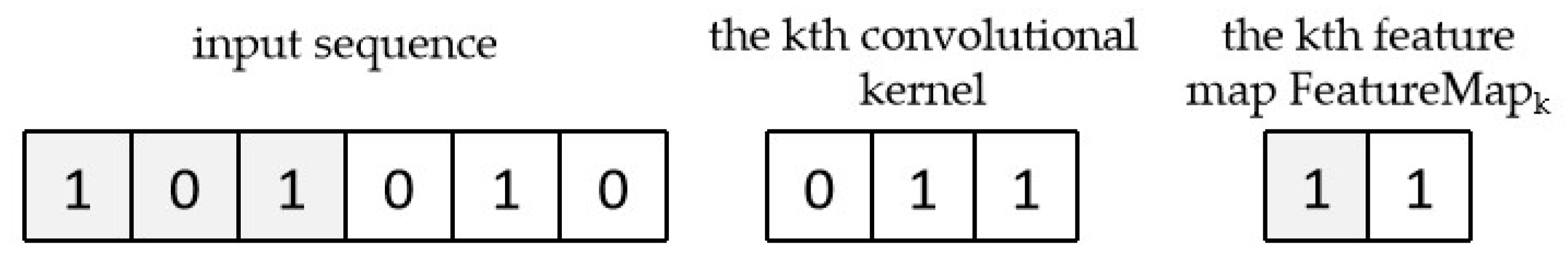
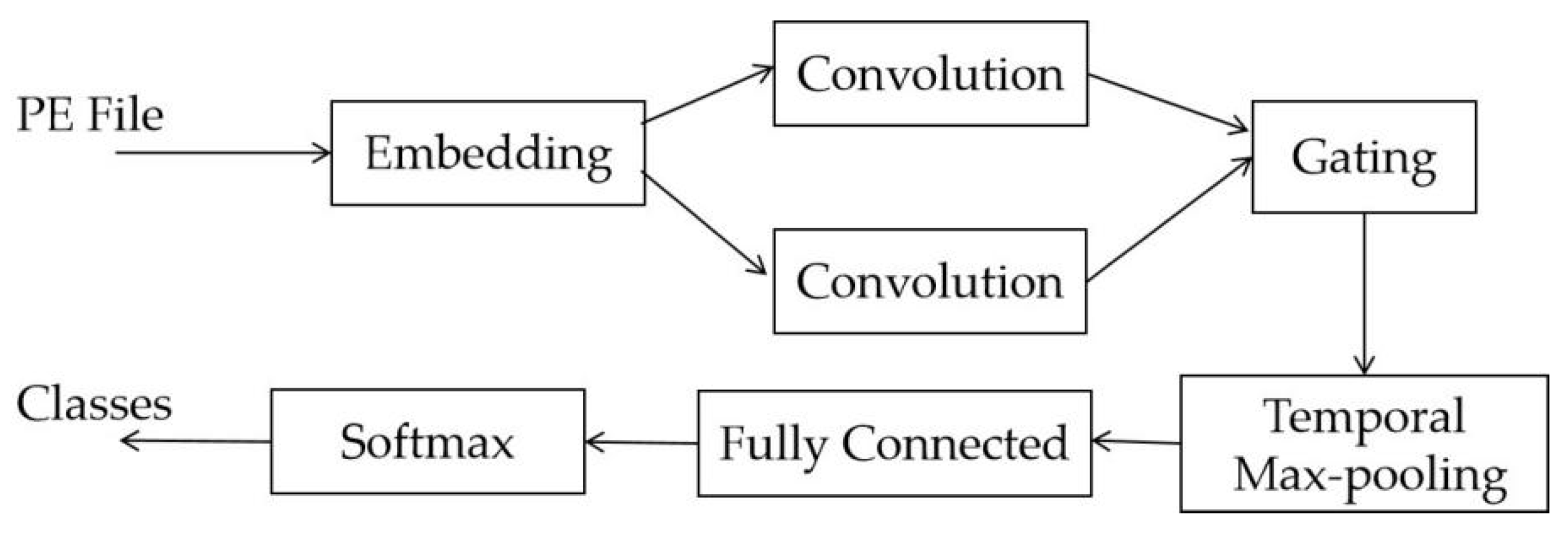
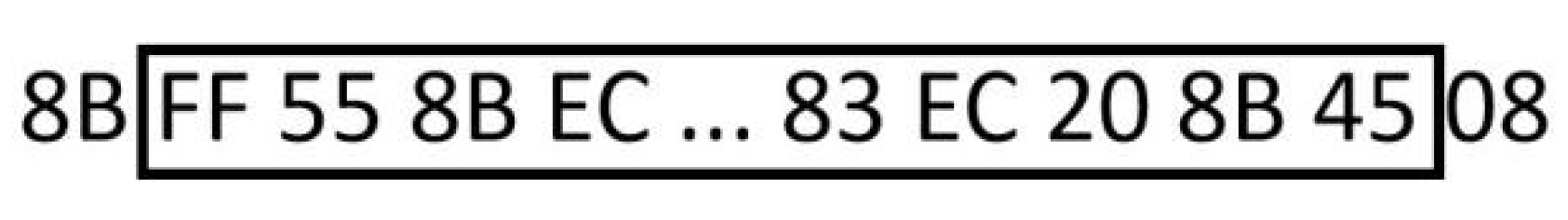
3.2. Finding Data Area Important for Classification

To evade the detection of malware detectors, we need to inject padding bytes into a source malware binary to change its category. To avoid using gradient-based algorithms to calculate the values of injected padding bytes, the padding bytes we use are the byte sequences extracted from benign executables. If these byte sequences can represent the characteristics of benign executables, the probability that an adversarial malware sample can fool a detector will increase. Therefore, our main task is to extract byte sequences which can represent the characteristics of benign executables.

To evade the detection of malware detectors, we need to inject padding bytes into a source malware binary to change its category. To avoid using gradient-based algorithms to calculate the values of injected padding bytes, the padding bytes we use are the byte sequences extracted from benign executables. If these byte sequences can represent the characteristics of benign executables, the probability that an adversarial malware example can fool a detector will increase. Therefore, our main task is to extract byte sequences which can represent the characteristics of benign executables.

CNN-based detectors generate explicit feature maps for input samples. Figure 1 gives an example for CNN convolution operation. The input data is a sequence. When we apply convolution to the input data, we mix two buckets of information. The first bucket is the input data. The second bucket is the convolution kernel, a single matrix of floating-point numbers. The output of the kernel is the altered sequence which is often called a feature map. Usually there are multiple convolution kernels and each kernel outputs a feature map. Feature maps represent features of an input data at different level. Through analyzing feature maps, we can discover which features are more important for decision making, and the data corresponding to important features can be used to construct adversarial samples.

Figure 1. Convolution of a sequence with a convolution kernel.

Grad-CAM [27] algorithm provides explanations for decisions from a large class of CNN-based models. We use the Grad-CAM algorithm to evaluate the important values of each feature map for a target class $c$. The important value of a feature map, with respect to a specific class is computed as Equation (1). ${\alpha }_k^c$ indicates the importance of $FeatureMa{p}_k$, with respect to class $c$.

$${\alpha }_k^c=\frac{1}{Len\_FeatureMa{p}_k}{\displaystyle \sum }_i\frac{\partial S^c}{\partial FeatureMa{p}_k\left[i\right]}$$

(1)

where $FeatureMa{p}_k$ is the $k$th feature map, $FeatureMa{p}_k\left[i\right]$ is the $i$th element of $FeatureMa{p}_k$, $Len\_FeatureMa{p}_k$ is the number of elements of $FeatureMa{p}_k$, $c$ is a class label, $S^c$ is the input for class $c$ in the softmax layer (classification layer in a CNN).

To discover the importance area of the input data for class $c$, the contributions of all feature maps need to be considered. The weighted sum of all feature maps is computed, which is defined as Equation (2). $L^c$ is called the class-discriminative localization map, which has the same size as a feature map.

$$L^c=\mathrm{ReLU}({\displaystyle \sum }_k{\alpha }_k^{c}FeatureMa{p}_k)$$

(2)

In (2) the ReLU function ($\mathrm{ReLU}\left(x\right)=\mathrm{Max}\left(0,x\right)$) is applied to the linear combination of feature maps because only the features that have a positive impact on class $c$ are considered. Without the ReLU function, the localization map sometimes highlights more than just the class of interest and performs worse at localization. Each element $L^c\left[i\right]$ can be seen as a feature extracted from the input data. The element $L^c\left[i\right]$, with a greater value, will also have more positive impact on class $c$. We can find the data area that is important for class $c$ by mapping $L^c\left[i\right]$ back to the corresponding data area in the input.

3.3. Generating Adversarial Examples

In reality the structure and parameters of a malware detector are unknown. In order to obtain the feature maps, we have to create a pseudo detector, which can simulate the true detector. MalConv [3] is a typical CNN-based detector. In our work, we select MalConv network as the pseudo detector. The network structure of MalConv is shown in Figure 2.

Figure 2. Structure of MalConv.

We regard an executable (PE file) as a byte stream. The input of MalConv is a fixed-length sequence from a PE file. If the length of an executable is shorter than the fixed-length, a number of zeros are inserted at the end of an executable. In MalConv, the first layer is an embedding layer, where each byte of an input sequence is converted into an 8-dimensional embedding vector. MalConv has two parallel convolutional layers. These embedding vectors are then transferred to two one-dimensional convolutional layers to generate feature maps, respectively. The next layer is a temporal max pooling layer, which combines the outputs of the two convolutional layers and passes them to a fully connected layer and a softmax layer for classification.

In our paper, we use Equation (1) to calculate the important value of each feature map, with respect to class $c$, denoted as ${\alpha }_{l,k}^c$, which is the important value of the $k$th feature map generated from the $l$th convolutional layer $FeatureMa{p}_{l,k}$. MalConv has two parallel convolutional layers. We normalize ${\alpha }_{l,k}^c$ for each independent convolutional layer, respectively, which is shown as Equation (3).

$$w_{l,k}^c=\frac{{\alpha }_{l,k}^c}{{{\displaystyle \sum }}_k{\alpha }_{l,k}^c}$$

(3)

The class-discriminative localization map is calculated as the weighted sum of the feature maps generated by the two parallel convolutional layers, which is shown as Equation (4). Here, we set all convolution kernels to have the same size; thus, all feature maps, as well as the class-discriminative localization map, have the same size, which are one-dimensional vectors. Different CNN-based networks have different structures. Another key problem we should resolve is how to locate the byte sequences in a source binary file, according to the class-discriminative localization map.

$$L^c=\mathrm{ReLU}({\displaystyle \sum }_l{\displaystyle \sum }_k{w}_{l,k}^{c}FeatureMa{p}_{l,k})$$

(4)

A MalConv model has two independent convolutional layers, and each convolution layer has multiple convolution kernels. To simplify data mapping, we set the kernel length equal to the kernel’s moving stride, all kernels have the same length, and the length of the input data is $2\times {10}^6$ bytes. The mapping relationship between a feature map and an input data can be constructed as follows.

In [3], the authors tried different parameter settings to test the performance of MalConv. We followed [3] and set the length and the moving stride of a kernel as 500, and the kernel number of each convolutional layer as 128. Figure 3 shows the relationships between an input data and a features map. In Figure 3, each square in the first row represents an input byte, and each square in the second row represents the embedding vector of an input byte. Kernel1 is a one-dimensional convolution kernel of a convolutional layer, whose length is 500. Kernel1 is convolved across the embedding data, computing the dot product between the entries of the kernel and the embedding data and producing a one-dimensional feature map $FeatureMa{p}_1$. If each convolutional layer has 128 kernels, we can obtain 128 one-dimensional feature maps from one convolutional layer. The embedding data has the same length as the input data. Therefore, each feature map has 4000 elements. In Figure 3, the fourth row shows the mapping relationship between an element of a feature map and a byte sequence in the input data. For example, the first element of $FeatureMa{p}_1$, $FeatureMa{p}_{1 }\left[1\right]$, is calculated by convoluting Kernel1 with the first five hundred elements of the embedding vector, and each input byte corresponds to an element of the embedding vector. Therefore, $FeatureMa{p}_1$ [1] is related with the first five hundred bytes of the input data. The class-discriminative localization map is the weighted sum of all feature maps, so it has the same mapping relationship as that of a features map.

Figure 3. Mapping feature map back to raw data.

To generate adversarial examples, we firstly train a MalConv model as the pseudo detector. Then, we create a dataset for feature extraction. All samples in the dataset are benign samples and can be correctly classified as benign by a detector. We input a sample to the pseudo detector and obtain the class-discriminative localization map $L^c$ of the sample. According to the mapping relationship between input data and the class-discriminative localization map, we can extract the byte sequences from the input data, which can represent the features of a sample. We usually extract the byte sequences corresponding to the elements having the greatest value in $L^c$. We call these byte sequences as feature byte sequences, which can be stored and shared by different adversarial samples. When generating an adversarial example, we randomly select one or multiple sequences and inject them into a malware sample.

Different from adversarial samples of image, feature byte sequences injected into a malware sample should have concrete program semantics. Sometimes the head and tail of a feature byte sequences are separated from other bytes of a program and cannot represent complete program semantics. In this case, we should extend a feature byte sequence to include the separate parts. For example, a feature byte sequence (bytes in the box), extracted according to the mapping relationship, is shown in Figure 4. The decompiling codes of the binary bytes are shown in Figure 5. We can see the head byte FF and the tail byte 45 cannot represent correct program semantics. To generate a feature byte sequence having correct program semantics, we should extend the feature byte sequences to include 8B and 08. From this point we can see the injected byte sequences, generated using our method, are explainable.

Figure 4. A sample of a feature byte sequence.

Figure 5. Decompiling codes of a binary byte sequence.

To more accurately locate the important area in the input data, we train several MalConv models with different parameter settings and combine the class-discriminative localization map from all MalConv models to locate the important area of the input data.

Algorithm 1 gives the algorithm for extracting feature byte sequences from input data using multiple detection models. The length of convolution kernels in different MalConv models can be different. For the convenience of extracting feature byte sequences, we define a new data structure $byteWeightMap$. It is a vector having the same length as the input data. Each element in $byteWeightMap$ records the important value of the corresponding byte of the input data. The important values of input bytes are assigned according to $L^c$. According to the mapping relationship, we can find the byte sequence corresponding to $L_i^c$ (the $i$th element of $L^c$); then, the values of the elements of $byteWeightMap$ corresponding to the byte sequence are set as $L_i^c$. The function $SetByteWeight()$ implements this objective. Due to multiple models used to locate feature byte sequences, we use $L_i^c$ and $byteWeightMa{p}_i$ represent the class-discriminative localization map and $byteWeightMap$, generated from model $M_i$ (the $i$th detector). The vector $fByteWeightMap$ is the sum of all $byteWeightMa{p}_i$, which stores the final important value of each byte of the input data.

In Algorithm 1, $ModelNum$ is the number of models, and $thresh$ gives the threshold of important value for selecting feature sequences. $x_{benign}$ is the input data. The function $GetFeatureMap()$ returns all the feature maps generated by model $M_i$. $FeatureMa{p}_{j,k}\left[n\right]$ is the $n$th element of the $k$th feature map generated by the $j$th convolutional layer of a MalConv model. The function $ExtFeaSeq()$ extracts all bytes whose important values are bigger than $thresh$ from $x_{benign}$, according to vector $fByteWeightMap$. The continuous bytes, having the same important value, consist of a feature byte sequence. Figure 6 shows a sample how to extract feature byte sequences from input data. We set $thresh$ as 50; therefore, only two feature byte sequences (sequences in black box) are extracted from input data.

Figure 6. Extracting feature byte sequences.

Algorithm 1: Extracting feature byte sequences of a benign sample.

Input:$x_{benign}, c=benign, M_1,\cdots ,M_{ModelNum}, ModelNum, thresh$

Output:$featureByteSequenceArray[]$

$fByteWeightMap=\overrightarrow{0};$

$\mathbf{for} i =1 \mathrm{to} ModelNum \mathbf{do}$

$\hspace{1em}\hspace{1em}\hspace{1em}\hspace{1em}\hspace{1em}\hspace{1em}\hspace{1em}FeatureMapArray=GetFeatureMap\left(M_i,x_{benign}\right);$

$WeightVector=\overrightarrow{0};$

$\mathbf{for} \mathrm{each} FeatureMa{p}_{j,k} \mathrm{in} FeatureMapArray \mathbf{do}$

${\alpha }_{j,k}^c=\frac{1}{Len\_FeatureMa{p}_{j,k}}{\displaystyle \sum }_n\frac{\partial S^c}{\partial FeatureMa{p}_{j,k}\left[n\right]};$

$\mathbf{end}$

$\hspace{1em}\mathbf{for} \mathrm{each} {\alpha }_{j,k}^c \mathbf{do}$

$\hspace{1em}{w}_{j,k}^c=\mathrm{Normalize}({\alpha }_{j,k}^c);$

$\hspace{1em}WeightVector=WeightVector+w_{j,k}^{c}FeatureMa{p}_{j,k};$

$\hspace{1em}\mathbf{end}$

$\hspace{1em}{L}_i^c=\mathrm{ReLU}\left(WeightVector\right);$

$\hspace{1em}byteWeightMa{p}_i=SetByteWeight\left(L_i^c\right);$

$\hspace{1em}fByteWeightMap=fByteWeightMap+byteWeightMa{p}_i;$

$\mathbf{end}$

$featureByteSequence[]=ExtFeaSeq\left(fByteWeightMap,thresh,x_{benign}\right)$

3.4. Strategies for Injecting Feature Sequences

A malware adversarial sample should preserve the same semantics as that of a source file. It requires that any byte in the source executable cannot be changed. Therefore, feature sequences should be injected into the spare space of an executable, which cannot be executed by a computer. Two strategies can be adopted to locate spare space in an executable: mid-file and end-of-file injection. We apply both strategies to generate adversarial samples in our work.

Mid-file injection: we locate the gaps between neighboring PE sections by parsing a PE file header. The gaps are placed by the compiler, since the physical size allocated to a PE section is greater than its virtual size. The length of a gap is calculated as RawSize-VirtualSize. The index of the start address of a gap is computed as PointerToRawData (offset address of a section) + VirtualSize. We collect the start address and length of each gap in an executable, then inject the feature byte sequences with appropriate length into these gaps.

End-of-file injection: another strategy we use is adding new sections at the end of a PE file and injecting feature byte sequences into the newly added sections. Since the new sections are not accessed by program code, the semantics of the original PE file are preserved. The process of adding a new section block includes three steps. First, we modify the value of bytes, which store the number and size of sections in the PE file header and update the values of file alignment and section alignment. Then, we use the offset address of the last section block plus the offset address of the new block as the final offset address. Next, we set the attribute values of the new section, such as the section name, execution attributes, size of the hard disk, and size of the memory. Finally, we modify the offset address of the aligned section and the offset address of the file in the section table and modify the size of image in the PE header.

Similar to [17], our method adopting the mid-file injection generates adversarial samples by injecting perturbed bytes in the gaps between neighboring PE sections. The method adopting end-of-file injection generates malware adversarial examples by adding new sections at the end of PE file, which is similar to previous methods [7,16,22,24]. However, all these methods [7,16,17,22,24] are belong to gradient-based method, which is optimized by computing the gradient of the objective function, with respect to each byte of a source malware binary. The gradient-based algorithm is an iterative algorithm and only one byte value is computed per iteration. Generating an adversarial malware sample by gradient-based method spends much time, so it is not applicable for generating a large number of adversarial samples. To avoid using gradient-based algorithms to calculate the values of injected padding bytes, our methods use the byte sequences extracted from benign executables to generate adversarial samples. In addition, our methods aim to evade CNN-based malware detectors, which is similar to [23]. We make a more detailed comparison between our method and the gradient-based method [16] in Section 4 and Section 5.

4. Experiments

4.1. Dataset Description

The malware samples we used came from the VirusShare project at http://virusshare.com/ (accessed on 1 December 2021). We downloaded 20,000 malicious samples, whose sizes were between 1 KB and 5 MB. The benign samples were collected from Windows platforms. We collected 20,000 benign Windows PE files in total. Two criteria were used to assess the quality of adversarial samples. The successful rate (SR) of the adversarial attack is defined as the percentage of the adversarial samples that can evade a detector. Another is the time cost for generating adversarial samples, which is used to evaluate the efficiency of the proposed algorithm. The experimental environment was 64-bit Ubuntu14 operating system, CPU Intel ^® Xeon Silver 4116 with 256 G memory.

4.2. Experimental Results

In the experiments, we trained four MalConv detectors. The description of parameter setting, training data, and detection accuracy is shown in Table 1. In Table 1, the column “Kernel Number” gives the kernel number for each convolutional layer. The training samples included fifty percent benign files and fifty percent malicious files, i.e., 5000 benign files and 5000 malicious files. The accuracy is defined as the percentage of the testing samples that can be correctly classified.

Table 1. Parameter setting for detectors.

Detector	Kernel Length	Moving Stride	Kernel Number	Training Samples	Accuracy
MalConv1	200	200	200	20,000	92.5%
MalConv2	400	400	150	20,000	92.6%
MalConv3	500	500	128	20,000	94.1%
MalConv4	800	800	100	20,000	91.8%

To objectively evaluate the successful rate that adversarial examples evade detection, in each experiment, we selected one MalConv model as the detector and used the remaining models to generate feature byte sequences. We repeated the experiments four times and used the average successful rate of four experiments to evaluate the performance of the proposed method. For each experiment, we randomly chose 100 benign samples from the testing set and use Algorithm 1 to extract the features sequences from benign samples. Only the sequences with the highest important value in each sample were selected. We got about two thousand feature sequences per experiment. We randomly selected 1000 samples that were correctly classified as malware from the testing set and injected feature sequences into them, in order to generate adversarial samples.

To observe how the number of injected bytes affects the performance of the proposed method, we injected different numbers of bytes into a sample. The number of the injected bytes was set to 1000, 2000, 5000, 10,000, and 20,000, respectively. In our work, two injection strategies were applied to inject feature byte sequences.

The experimental results, adopting the mid-file and the end-of-file strategies, are shown in Table 2 and Table 3, respectively. In two tables, “Avg Time Cost Per Sample” means the time cost for generating an adversarial sample.

Table 2. SR of the proposed method adopting the mid-file strategy.

No. of Injected Bytes	1000	2000	5000	10,000
SR of Experiment 1	0.42	0.55	0.78	0.88
SR of Experiment 2	0.46	0.57	0.77	0.86
SR of Experiment 3	0.45	0.59	0.78	0.90
SR of Experiment 4	0.41	0.61	0.76	0.89
Average SR	0.44	0.58	0.77	0.88
Avg Time Cost Per Sample(min)	0.2	0.5	1.1	2.1

Table 3. SR of the proposed method adopting the end-of-file strategy.

No. of Injected Bytes	1000	2000	5000	10,000	20,000
SR of Experiment 1	0.34	0.41	0.60	0.77	0.88
SR of Experiment 2	0.37	0.44	0.61	0.73	0.90
SR of Experiment 3	0.32	0.40	0.64	0.74	0.91
SR of Experiment 4	0.33	0.43	0.63	0.76	0.87
Average SR	0.34	0.42	0.62	0.75	0.89
Avg Time Cost Per Sample(min)	0.2	0.2	0.4	0.9	1.9

To verify whether the feature sequences can represent the characteristics of benign executables, we compared the proposed method with the randomly injecting method. The randomly injecting method randomly extracts byte sequences from benign executables and injects them into malware to generate adversarial samples. For the randomly injecting methods, we also used two different strategies to inject randomly extracted sequences. The experimental results are shown in Table 4 and Table 5, respectively.

Table 4. SR of the randomly injecting method adopting mid-file strategy.

No. of Injected Bytes	1000	2000	5000	10,000
SR of Experiment 1	0.09	0.11	0.18	0.21
SR of Experiment 2	0.09	0.11	0.17	0.20
SR of Experiment 3	0.06	0.13	0.15	0.24
SR of Experiment 4	0.08	0.13	0.14	0.23
Average SR	0.08	0.12	0.16	0.22

Table 5. SR of the randomly injecting method adopting end-of-file strategy.

No. of Injected Bytes	1000	2000	5000	10,000	20,000
SR of Experiment 1	0.03	0.07	0.07	0.10	0.18
SR of Experiment 2	0.05	0.05	0.09	0.12	0.15
SR of Experiment 3	0.03	0.06	0.09	0.11	0.16
SR of Experiment 4	0.05	0.06	0.07	0.11	0.19
Average SR	0.04	0.06	0.08	0.11	0.17

From Table 2, Table 3, Table 4 and Table 5, we can see that the successful rate of the proposed method was significantly higher than that of the randomly injecting method, which was about 30%–60% higher than that of the corresponding randomly injecting method. It proves that the feature sequences injected into adversarial samples can reflect the characteristics of benign executables, which can influence the decision of the detectors. The injected sequences were extracted from benign executables. If more benign sequences were injected in a malware sample, a malware sample will be more similar as a benign sample. Therefore, we can see, for both methods, that the success rate increased with the length of the injected bytes increasing.

For the end-of-file strategy, all malicious features in malware samples are preserved and not modified. Compared with the end-of-file strategy, the mid-file strategy injects feature sequences into the gaps between sections, which destroys some malicious features of malware samples. To mislead the detector, the end-file strategy needs to inject more feature byte sequences to counteract the effects of the original malicious features. Therefore, from Table 2, Table 3, Table 4 and Table 5 we can see when injecting the same number of benign bytes into malware samples, the successful rate of the method adopting the mid-file strategy is higher than that adopting the end-of-file strategy. For the proposed method, the successful rate adopting the mid-file strategy is about 3–23% higher than that adopting the end-of-file strategy. For the randomly injecting method, the successful rate adopting the mid-file strategy is about 4–11% higher than that adopting the end-of-file strategy.

We also compare the proposed method with the gradient-based method [16]. The end-of-file strategy is adopted to inject feature sequences. For the gradient-based method, the gradient is calculated by minimizing the classification loss of the detector, with respect to the target label. In the experiment we select two different classification loss functions to calculate the gradient. One is the softmax classification loss (see Equation (5)), which is used to train MalConv. The other is the mean-square error (see Equation (6)), which is often used to train conventional back propagation (BP) networks.

$$L_{softmax}\left(\theta \right)=-\frac{1}{m}\left[{\displaystyle \sum }_{i=1}^m{\displaystyle \sum }_{j=1}^{k}1\{y^{\left(i\right)}=j\}log\frac{e^{{\theta }_j^T{x}^{\left(i\right)}}}{{{\displaystyle \sum }}_{l=1}^k{e}^{{\theta }_l^T{x}^{\left(i\right)}}}\right]$$

(5)

$$L_{ms}\left(\theta \right)=\frac{1}{2m}{{\displaystyle \sum }}_{i=1}^m{\left({\widehat{y}}_i-y_i\right)}^2$$

(6)

Due to the limitation of computing cost, only 200 adversarial samples are generated for each experiment and the maximum number of the injected bytes is less than 10,000. The experimental results adopting two different classification loss functions are shown in Table 6. We can see the successful rate of the proposed method adopting the end-of-file strategy is about 6–10 percent higher than that of the gradient-based method adopting softmax classification loss. The successful rate of the gradient-based method adopting softmax classification loss is about 5–17 percent higher than the method adopting mean squared error loss.

Table 6. SR of the gradient-based method [16].

	Softmax Classification Loss				Mean Squared Error
Byte seq. len.	1000	2000	5000	10,000	1000	2000	5000	10,000
Experiment 1	0.23	0.33	0.52	0.70	0.15	0.25	0.36	0.51
Experiment 2	0.26	0.39	0.55	0.66	0.21	0.27	0.40	0.49
Experiment 3	0.25	0.30	0.56	0.69	0.19	0.29	0.42	0.52
Experiment 4	0.22	0.32	0.53	0.71	0.22	0.30	0.41	0.54
Average SR	0.24	0.31	0.54	0.69	0.19	0.28	0.40	0.52
Avg Time Cost Per Sample(min)	25	51	99	239	23	47	100	240

5. Discussion

From the experiments we can see the gradient-based algorithm takes a relatively long time to generate an adversarial sample. In our work, 200 adversarial samples are generated for each experiment. The gradient-based method takes an average about 100 min to generate an adversarial sample (See Table 6), because it only generates one appended byte per iteration. In addition, it is hard to determine the iteration number when appended bytes converge to their optimal values. If we use the gradient-based algorithm to generate a large amount of adversarial samples, the time cost is very high. For the proposed method, most time is spent on training a CNN-based detector. In the experiments, we spent about 10 h training a MalConv model. The time for extracting feature sequences is about one hour. Injecting feature sequences into a PE file can be done in a very short time (the average time in our experiment is about one minute, see Table 2 and Table 3). Because the feature sequences can be shared by all adversarial samples, the proposed method is suitable for generating a large number of adversarial samples.

Interpretability is another challenge faced by adversarial sample generation algorithms. The gradient-based methods calculate the value of injected bytes by minimizing the classification loss of a detector, with respect to the target label. These injected bytes have no explainable semantics and are only treated as binary values. Different from the gradient-based methods, the proposed method injects feature byte sequences into malware. A feature sequence is a byte sequence extracted from a benign executable. By decompiling the executable, the semantics of a feature byte sequences can be clearly defined. Therefore, using the proposed method we can explain the meaning of the injected bytes.

In our study, the proposed method is only designed to generate the adversarial samples for CNN-based detectors. The feature byte sequences are selected based on the convolution operation of CNN. This means that we need to know in advance which algorithms a detector uses. Compared with our proposed method, the gradient-based methods are more commonly used methods, which do not assume the classification methods a detector uses. So, they can be more widely used to generated adversarial samples for different neural networks, such as BP network, CNN [16], and RNN [20].

Generating malware adversarial samples is different from generating image adversarial samples. For image adversarial samples, we can directly update each pixel. For malware adversarial samples, we cannot modify any byte of a source executable, otherwise we cannot guarantee that it can be executed correctly. Therefore, we have to inject padding bytes into the gaps or the end of a PE file. The number of gaps and the length of each gap in a PE file are limited. Using the mid-file strategy, sometimes we cannot find enough gaps to store feature byte sequences in an executable, which may reduce the successful rate. For the end-of-file strategy, we can append any number of section blocks at the end of a PE file by modifying the PE file structure. Therefore, it is relatively easy for the end-file strategy to inject enough bytes to generate an adversarial sample. However, adversarial samples generated using the end-of-file strategy are prone to be detected by simply analyzing the PE section table or examining if such sections are accessed by program instructions. In addition, if the length of a malware sample is greater than the input length of a detector, and the end-of file strategy cannot be applied.

6. Conclusions

In this paper we study how to generate malware adversarial samples. Different from previous gradient-based methods, we generate malware adversarial examples by injecting byte sequences into a source executable. The injected byte sequences can be shared by different adversarial samples. Our proposed method is efficient and suitable for generating a large number of adversarial samples. We proposed the algorithm to extract feature byte sequences for CNN-based deep learning models. Feature byte sequences can represent the characteristics of benign samples. Compared with the padding bytes generated using gradient-based methods, the feature byte sequences are explainable. The experimental results show that the adversarial samples, generated using the proposed method, have a high successful rate, and the proposed method is suitable for generating a large number of adversarial samples. It is possible that a more robust malware detector can be trained using the generated adversarial samples and the original samples. In this work, we have not yet provided definitive evidence for the benefits of the generated adversarial samples in improving performance of malware detection, due to the complexity of adversarial training malware detectors. In our future work, we plan to investigate how to use the generated adversarial malware samples to improve the performance of malware detection models.

References

1. Alzaylaee, M.K.; Yerima, S.Y.; Sezer, S. DL-Droid: Deep learning based android malware detection using real devices. Comput. Secur. 2020, 89, 101663. [Google Scholar] [CrossRef]
2. Gibert, D.; Mateu, C.; Planes, J. HYDRA: A multimodal deep learning framework for malware classification. Comput. Secur. 2020, 95, 101873. [Google Scholar] [CrossRef]
3. Raff, E.; Barker, J.; Sylvester, J.; Brandon, R.; Catanzaro, B.; Nicholas, C.K. Malware detection by eating a whole exe. In Proceedings of the Workshops at the Thirty-Second AAAI Conference on Artificial Intelligence, New Orleans, LA, USA, 2–7 February 2018; pp. 268–276. [Google Scholar]
4. Wang, W.; Zhao, M.; Wang, J. Effective android malware detection with a hybrid model based on deep autoencoder and convolutional neural network. J. Ambient Intell. Humaniz. Comput. 2019, 10, 3035–3043. [Google Scholar] [CrossRef]
5. Szegedy, C.; Zaremba, W.; Sutskever, I.; Bruna, J.; Erhan, D.; Goodfellow, I.; Fergus, R. Intriguing properties of neural networks. arXiv 2013, arXiv:1312.6199. [Google Scholar]
6. Biggio, B.; Nelson, B.; Laskov, P. Support Vector Machines Under Adversarial Label Noise. J. Mach. Learn. Res. 2011, 20, 97–112. [Google Scholar]
7. Suciu, O.; Coull, S.E.; Johns, J. Exploring adversarial examples in malware detection. In Proceedings of the 2019 IEEE Security and Privacy Workshops (SPW), San Francisco, CA, USA, 20–22 May 2019; pp. 8–14. [Google Scholar]
8. Maiorca, D.; Demontis, A.; Biggio, B.; Roli, F.; Giacinto, G. Adversarial detection of flash malware: Limitations and open issues. Comput. Secur. 2020, 96, 101901. [Google Scholar] [CrossRef]
9. Goodfellow, I.J.; Shlens, J.; Szegedy, C. Explaining and Harnessing Adversarial Examples. arXiv 2014, arXiv:1412.6572. [Google Scholar]
10. Goodfellow, I. New CleverHans Feature: Better Adversarial Robustness Evaluations with Attack Bundling. arXiv 2018, arXiv:1811.03685. [Google Scholar]
11. Moosavi-Dezfooli, S.M.; Fawzi, A.; Frossard, P. DeepFool: A simple and accurate method to fool deep neural networks. In Proceedings of the 2016 IEEE Conference on Computer Vision and Pattern Recognition (CVPR), Las Vegas, NV, USA, 27–30 June 2016; pp. 2574–2582. [Google Scholar]
12. Papernot, N.; McDaniel, P.; Jha, S.; Fredrikson, M.; Celik, Z.B.; Swami, A. The limitations of deep learning in adversarial settings. In Proceedings of the 2016 IEEE European Symposium on Security and Privacy (EuroS&P), Saarbrücken, Germany, 21–24 March 2016; pp. 372–387. [Google Scholar]
13. Xiao, H.; Xiao, H.; Eckert, C. Adversarial label flips attack on support vector machines. In Proceedings of the 20th European Conference on Artificial Intelligence (ECAI 2012), Montpellier, France, 27–31 August 2012; pp. 870–875. [Google Scholar]
14. Papernot, N.; McDaniel, P.; Goodfellow, I.; Jha, S.; Celik, Z.B.; Swami, A. Practical black-box attacks against machine learning. In Proceedings of the 2017 ACM on Asia Conference on Computer and Communications Security, Abu Dhabi, United Arab Emirates, 2–6 April 2017; pp. 506–519. [Google Scholar]
15. Liu, Y.; Chen, X.; Liu, C.; Song, D. Delving into transferable adversarial examples and black-box attacks. arXiv 2016, arXiv:1611.02770. [Google Scholar]
16. Kolosnjaji, B.; Demontis, A.; Biggio, B.; Maiorca, D.; Giacinto, G.; Eckert, C.; Roli, F. Adversarial malware binaries: Evading deep learning for malware detection in executables. In Proceedings of the 2018 26th European Signal Processing Conference (EUSIPCO), Rome, Italy, 3–7 September 2018; pp. 533–537. [Google Scholar]
17. Kreuk, F.; Barak, A.; Aviv-Reuven, S.; Baruch, M.; Pinkas, B.; Keshet, J. Deceiving end-to-end deep learning malware detectors using adversarial examples. arXiv 2018, arXiv:1802.04528v3. Available online: http://arxiv.org/abs/1802.04528v3 (accessed on 1 December 2021).
18. Hu, W.; Tan, Y. Generating adversarial malware examples for black-box attacks based on GAN. arXiv 2017, arXiv:1702.05983. [Google Scholar]
19. Al-Dujaili, A.; Huang, A.; Hemberg, E.; O’Reilly, U.M. Adversarial deep learning for robust detection of binary encoded malware. In Proceedings of the 2018 IEEE Security and Privacy Workshops (SPW), San Francisco, CA, USA, 21–23 May 2018; pp. 76–82. [Google Scholar]
20. Hu, W.; Tan, Y. Black-box attacks against RNN based malware detection algorithms. In Proceedings of the Workshops at the Thirty-Second AAAI Conference on Artificial Intelligence, New Orleans, LA, USA, 2–7 February 2018; pp. 245–251. [Google Scholar]
21. Chen, S.; Xue, M.; Fan, L.; Hao, S.; Xu, L.; Zhu, H.; Li, B. Automated poisoning attacks and defenses in malware detection systems: An adversarial machine learning approach. Comput. Secur. 2018, 73, 326–344. [Google Scholar] [CrossRef] [Green Version]
22. Kreuk, F.; Barak, A.; Aviv-Reuven, S.; Baruch, M.; Keshet, J. Adversarial examples on discrete sequences for beating whole-binary malware detection. arXiv 2018, arXiv:1802.04528v1. Available online: http://arxiv.org/abs/1802.04528v1 (accessed on 1 December 2021).
23. Peng, X.; Xian, H.; Lu, Q.; Lu, X. Semantics aware adversarial malware examples generation for black-box attacks. Appl. Soft. Comput. 2021, 109, 107506. [Google Scholar] [CrossRef]
24. Chen, B.; Ren, Z.; Yu, C.; Hussain, I. Adversarial examples for cnn-based malware detectors. IEEE Access 2019, 7, 54360–54371. [Google Scholar] [CrossRef]
25. Chen, J.; Jiang, J.; Li, R.; Dou, Y. Generating adversarial examples for static PE malware detector based on deep reinforcement learning. In Proceedings of the 5th Annual International Conference on Information System and Artificial Intelligence (ISAI2020), Hangzhou, China, 22–23 May 2020. [Google Scholar]
26. Krčál, M.; Švec, O.; Bálek, M.; Jašek, O. Deep convolutional malware classifiers can learn from raw executables and labels only. In Proceedings of the 6th International Conference on Learning Representation (ICLR 2018), Vancouver, BC, Canada, 30 April–3 May 2018. [Google Scholar]
27. Selvaraju, R.R.; Das, A.; Vedantam, R.; Cogswell, M.; Parikh, D.; Batra, D. Grad-CAM: Why did you say that? Visual Explanations from Deep Networks via Gradient-based Localization. In Proceedings of the IEEE International Conference on Computer Vision, Venice, Italy, 22–29 October 2017; pp. 618–626. [Google Scholar]
Publisher’s Note: MDPI stays neutral with regard to jurisdictional claims in published maps and institutional affiliations.
Article Metrics
Citations
Article Access Statistics
Multiple requests from the same IP address are counted as one view.