Acoustic Anomaly Detection of Mechanical Failures in Noisy Real-Life Factory Environments

Abstract

Anomaly detection without employing dedicated sensors for each industrial machine is recognized as one of the essential techniques for preventive maintenance and is especially important for factories with low automatization levels, a number of which remain much larger than autonomous manufacturing lines. We have based our research on the hypothesis that real-life sound data from working industrial machines can be used for machine diagnostics. However, the sound data can be contaminated and drowned out by typical factory environmental sound, making the application of sound data-based anomaly detection an overly complicated process and, thus, the main problem we are solving with our approach. In this paper, we present a noise-tolerant deep learning-based methodology for real-life sound-data-based anomaly detection within real-world industrial machinery sound data. The main element of the proposed methodology is a generative adversarial network (GAN) used for the reconstruction of sound signal reconstruction and the detection of anomalies. The experimental results obtained in the Malfunctioning Industrial Machine Investigation and Inspection (MIMII) show the superiority of the proposed methodology over baseline approaches based on the One-Class Support Vector Machine (OC-SVM) and the Autoencoder–Decoder neural network. The proposed schematics using the unscented Kalman Filter (UKF) and the mean square error (MSE) loss function with the L2 regularization term showed an improvement of the Area Under Curve (AUC) for the noisy pump data of the pump.

1. Introduction

Anomaly detection, or novelty detection, is a well-studied topic in data science [1] with various applications. The technique has recently received further attention due to the development of the Internet of Things (IoT) and the following explosive growth of big data and to rapid improvement of machine learning techniques, especially deep learning, in the last decade. Anomaly detection is recognized as one of the essential techniques in an application for preventive maintenance of the industrial machine [2] as well as for predictive maintenance of useful life (or time to failure) [3] and quality control [4]. Anomaly detection of industrial machinery relies on various diagonal data from equipped sensors, such as temperature, pressure, electric current, vibration, and sound, to name a few. Among these data, sound data are easy to collect in the factory due to the relatively low installation cost of microphones to existing facilities, and various approaches have been studied [5,6,7,8].

Failure sounds can be associated with a distinguishable fault sound signature, varying in a dedicated frequency range and harmonics. For example, low-frequency range is often a factor in defining shifts in rotational speed up to lower harmonics, containing information about unbalance, misalignment, failing bearing, and general mechanical construction shifts. The medium frequency range can be used to define failure in multipart mechanisms, such as gearboxes, indicating wear or an upcoming failure by a shift in its harmonics. High frequency ranges, for example, can indicate steam flow or other similar failure. Often the noises are so varying in their characteristics (e.g., railway sounds) that they become “unconventional noises” and are usually neglected in noise modelling [9]. The key problem and the main subject of this study is the real-life case of noisy environments drowning these failure sounds. Suddenly, these noise characteristics become hard to detect as background noise. This is known to exacerbate diagnosis, and the fact that the sound data can be readily contaminated by environmental sound makes the application of sound data-based anomaly detection complicated. Therefore, the development of a noise-tolerant machine learning methodology is crucial for the application of sound-data-based anomaly detection in a real factory. We believe that a side effect of such a “feature hunt” in extremely noise-contaminated signals can also benefit human well-being studies, as was found in the case of analyzing noise-contaminated environments signals of noise contaminated environments inducing annoyance [10] affecting work performance [11,12] and learning [13], and leading to cognitive performance decline [14] and even increased blood pressure [15], hypertension [16] or myocardial infarction [17].

The main objective of the study is to improve the accuracy in classifying normal and anomalous conditions of industrial machines based on noisy sound data by proposing a novel model and algorithm for anomaly detection from industrial noisy data.

The paper is structured as follows. In Section 2, we provide an overview of precedent works related to anomaly detection using machine learning and deep learning. In Section 3, we describe the dataset and our methodology. In Section 4, we provide an outline of the experiments conducted and the results achieved. In Section 5, we present a comparison with other work and discussion. In Section 6, we conclude by pointing out the directions for further work.

2. Related Works

In this section, we describe anomaly detection techniques using machine learning. Anomaly detection addresses the problem of discovering patterns in data that do not replicate the expected behavior [18]. These non-standard patterns are called anomalies, outliers, and exceptions. No matter how it is called, the common principle is to measure the extent of the difference between normal and anomalous data numerically.

2.1. Analysis of Industrial Machinery Data for Predictive Maintenance

The majority of existing production lines’ equipment can provide valuable data, which may then be examined and the resulting knowledge applied more efficiently. The standard preventive maintenance becomes predictive because of this knowledge. This strategy, known as Maintenance 4.0, may therefore better address issues that develop, including those that are not known ahead of time. Predictive maintenance (PdM) [19] is one of the key components of Maintenance 4.0, while one of the crucial parts of PdM is anomaly detection, which can be applied, for example, on the temperature characteristic of the technological process measured in real-time and analyzed using a neural network [20], or by monitoring the sounds produced by the milling process using spectral analysis and K-means clustering algorithms [21]. When applied in an unsupervised way, the approach can be used for predicting the remaining useful life in the absence of available run-to-failure data, as was done in [22] using the autoencoder based methodology to analyze the vibrations of a robotic arm. Skoczylas et al. [23] used a diagnostic feature extracted from the spectral coefficients of the acoustic signal to identify the faulty operation of the rotating elements of the belt conveyor using the autocorrelation characteristics. Ho et al. [24] suggested using Blind Source Separation as a signal decomposition approach to analyze vibration data of rotating bearings for the detection of fault patterns and signatures. Mey et al. [25] adopted a step-by-step integration of classifications obtained from vibration and acoustic emission sensors to incorporate information from low and high frequency signals collected from a system of a motor train and bearings with some artificial damages. The results show that utilizing the suggested approach of integrating classifiers for vibrations and acoustic emissions, damage classification may be improved. Serradilla et al. [26] employed the feature vector of the autoencoder’s latent space to cluster data collected from a press machine of a stamping production line. The explainable artificial intelligence techniques were used to track the autoencoder’s loss on input data to detect anomalous work conditions. More works on the analysis of vibration and acoustic data for early fault diagnostics of industrial machinery are discussed in the review paper [27,28].

From a technology perspective the problem of failure analysis is also related to the robust speaker identification methods, focusing on a segregation of sounds from different acoustics mixtures, especially in low quality signals [29]. Williamson et al. tackled this problem by applying an estimate of the real and imaginary components of the complex ideal ratio mask with a good performance versus more traditional methods [30]. This problem is particularly expressed in very noisy environments similar to those in our study. Ayhan et al. showed that by a combination of mask estimation, gammatone features with bounded marginalization dealing with unreliable features with a classic Gaussian mixture model may lead to an improvement in distinguishing the lead signal [31].

Several techniques and models have been proposed which should be selected considering the characteristics of the data, the behavior of anomalous data, and the purpose of the application. We categorize anomaly detection techniques into signal processing-based methods, machine learning methods, and deep learning methods.

2.2. Signal Processing Based Methods

Getting meaningful information from noisy data is a classical subject in the field of geoscience and medical sciences, to name a few, where the experimental data are usually low Signal-to-Noise Ratio (SNR) due to inevitable environmental noise. A prevalent noise reduction method is the application of the filter to the sample. Some types of filters, such as high-pass, band-pass, low-pass, and median filters [32], are utilized to select the designated frequency or amplitude. This technique is easy to build in and widely used in applications, but there is the risk to unintendedly eliminate necessary signals if the sound data has a low SNR or the sound data is unknown. One of the most typical methods for the detection of statistical anomaly detection is based on the control chart, with applications for the monitoring of industrial machine and bearing monitoring [33].

Another approach to noise reduction is based on multivariate analysis. Independent component analysis (ICA) [34] is a powerful idea for multivariant data that has been already utilized in the biomedical signal and image domain, such as electroencephalography and magnetic resonance imaging [35] and geosciences for train noise separation [36]. ICA relies on the underlying assumption that a received signal is a combination of mutually independent signals. The independence among the source signals is evaluated in the Kullback–Leibler cost function. ICA is formulated for noiseless cases; therefore, techniques for real-world data such as adding noise terms, which have mutually independent components, and using semiparametric approaches, were proposed [35]. Empirical mode decomposition (EMD) is another method for the analysis of multi-component signals that have been used to de-noise jitter noise in telecommunication signals [37]. Spectral analysis was applied in [38] to perform a vibration analysis of a fan motor. Random matrix theory was applied to the imaging of the sensor array imaging perturbed by measurement noise [39]. The theory assumes that the distribution of eigenvalue of a product of random matrix to itself is converged to the Marcenko–Pastur distribution at a large scale, and this can provide information of threshold for selecting signals and noise.

2.3. Machine Learning-Based Methods

Classification-based methods are generally supervised anomaly detection. In this approach, a model or classifier is trained from a set of labeled data instances, and the learned model is used to classify test instances. Both multiclass and one-class anomaly detection techniques are available. Multiclass anomaly detection is a technique that assumes that training data contains labeled instances that belong to multiple normal classes. The model has to learn a classifier to identify the normal class against all other classes. If test data are not classified as normal by any of the classifiers learned by the model, then they are considered an outlier. This technique gives their prediction a confidence score. Therefore, this technique applies to data whose normal classes are known.

The distribution-based method is used to model the distribution of normal data. The probabilistic model is used to identify data with a different distribution of its features. As the data space has high dimensionality, the distance cannot be measured in the Euclidean way and therefore various measurement methodologies were proposed, such as the Local Outlier Factor (LOF) as a density-based method [40], and the Nearest-Neighborhood as a distance-based method [41]. Hsu et al. [42] employed density-based spatial clustering of applications with noise algorithms to identify abnormal state in wind turbine data. Then, random forest and decision tree algorithms were used to construct to predict wind turbine anomalies. Toma et al. [43] suggested a hybrid technique that uses statistical features, genetic algorithms (GA), and machine learning models (KNN, random forest, and decision tree) to diagnose motor current faults.

These classical approaches are already recognized as proven techniques. If the input data are simple, these techniques are still the first choice for the application. However, complicated data such as image recognition community and audio processing may exceed the modeling assumptions of these machine learning techniques.

2.4. Deep Learning-Based Methods

The advent of deep learning techniques for anomaly detection has improved the results of traditional methods. Deep learning is based on an artificial neural network model. Deep learning promises to train hierarchical models that represent probability distributions over input data. The recent development in both hardware and neural models, especially in the last decade, has overcome the challenges, making artificial intelligence a thriving field with many practical applications and active research topics.

One of the successful methods using deep learning is a reconstruction-based method [44]. The fundamental idea behind the methods is that the normal condition can be reconstructed accurately from a reduced latent space interim of neural network architecture, whereas anomalous conditions cannot be reconstructed embracing larger reconstruction losses. This fashion is suitable for anomaly detection, where the volume of anomalous condition data is generally much smaller than normal condition data because a model for detection can be trained only using the normal condition data. Deep one-class (DOC) is an approach inspired by kernel-based one-class classification and minimum volume estimation and the training of a neural network while minimizing the volume of a hypersphere that encloses the network representations of the data [45]. Minimizing the volume of the hypersphere forces the network to extract the common factors of variation, and anomalies can be detected if the test instance is plotted out of the boundary of the hypersphere. Luwei et al. [46] used a two-stage ANN model for the classification of rotating machines faults based on real-life vibration data. Zhao et al. [47] used a deep autoencoder (DAE) network, model. The parameters of the model, acquired by learning normal operational supervisory control and data acquisition (SCADA) data from wind turbines, we used for fault detection of turbine components. Dongo et al. [48] suggested regression-based abnormality decision using manifold learning with autoencoder. The approach has been validated on the sound data of the operating machine. Cheng et al. [49] extracted the characteristics of the time, frequency, and time-frequency domain. Feature selection was performed using a Euclidean distance. Next, adaptive kernel spectral clustering (AKSC) was used to find machine anomaly behaviors, and deep long- and short-term memory recurrent neural networks (LSTM-RNN) were used to predict the failure time of the machine. Li et al. [50] proposed a Deep Small-World Neural Network (DSWNN) to detect early failures of wind turbines based on anomaly in turbine sensor data.

In summary of the related work, a general observation is that deep learning is expected to outperform traditional machine learning for anomaly detection in big data [51].

2.5. Generative Adversarial Network-Based Methods

The central idea of Generative adversarial networks (GAN) is that a generator trained with normal data poses high reconstruction loss when trying to generate an anomalous image. Discriminative models map a high-dimensional input to a class label for pattern recognition [52]. Anomaly detection using GANs emerged recently but has already shown promising performances, especially for big and complicated data. In the reconstruction context, GAN is also applied for anomaly detection (AnoGAN) [53,54]. For example, Wu et al. [55] suggested a probabilistic adversarial generative auto-encoder for machine fault classification of machines. We think these approaches are applicable for anomaly detection with audio data, as our concern is to measure the difference between normal and anomalous. Zhang et al. [56] proposed a multi-index generative adversarial network (MI-GAN) to detect tool wear from imbalanced sensor signal data.

3. Materials and Methods

3.1. Methodology

In this research, the purpose is to improve the robustness of anomaly detection in the domain of stationary valves and slide rails (Figure 1). Figure 2 illustrates the schematics of the network applied for anomaly detection in acoustic data. In the research, our experiments are carried out on the MIMII data set [57], as it is explained in further sections.

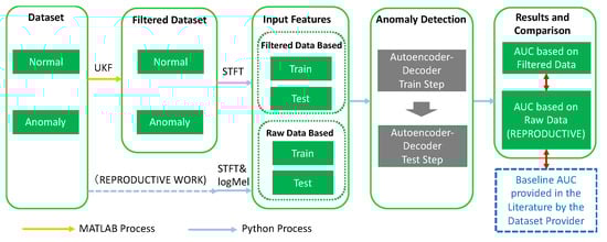
Figure 1. The workflow of experiment.

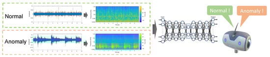
Figure 2. Illustration of a neural network applied for anomaly detection in acoustic data.

3.2. Datasets

In 2019, researchers at the Japanese manufacturing company Hitachi Co. Ltd. introduced a new dataset of Industrial Machine Inspection and Inspection Malfunction Investigation and Inspection (MIMII) [58]. The data set consists of four distinct types of machinery: valves, pumps, fans, and slide rails. The data set is provided in the waveform audio file (.wav) format. The audio data consist of machine sound and noise. The noise is real factory environment sound, and it is artificially mixed with the pure machine sound at several levels of signal-noise ratio (SNR): 6 dB, 0 dB, and −6 dB. The machine sound is recoded for both normal and abnormal conditions. There is no label on the abnormal condition sound data except that they explained the abnormal indicates various troubles. As a result, the characteristics of the data set can be described by the type of machinery and SNR. The machine sound is recorded in 16 (bit) at a sampling rate of 16,000 (Hz) and a.wav file is a segment of 10 (s); accordingly, the file of one segment consists of 160,000 samples of time frames. The list of pump sound files is reported in Table 1. The pump sound data set consists of four different pumps, labeled Model ID00, 02, 04, and 06. The number of segments for the normal condition of each machine is seven to ten times larger than that of the anomalous conditions.

Table 1. Contents of MIMII dataset.

Model ID	Segments for Normal Condition	Segments for Anomalous Condition
ID00	1006	143
ID02	1005	111
ID04	702	100
ID06	1036	102

3.3. Feature Engineering

The feature engineering in the experiment follows the recommendations of the data set provider, that is, each segment of waveform sound data is processed in Fast Fourier Transformation (FFT) and then applied the logMelspetctrogram. This process is shown illustratively in Figure 3.

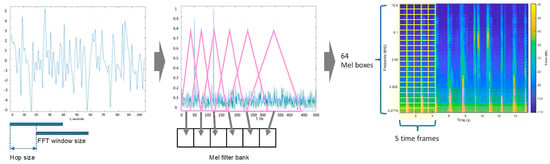
Figure 3. Schematics of the audio data process from time-frequency to log-Mel spectrogram.

The data set provider developed the input feature by combining five frames and made a 320-dimensional feature vector for the autoencoder. On the other hand, we have developed an input feature for a suitable format for models we are going to study.

3.4. Problem Formulation and Signal Processing

Let $X, {\mathcal{G}}_{\theta }$ as an STFT of signal (spectrogram in time-frequency space) and a filter with parameter theta, respectively:

$$G={\mathcal{G}}_{\theta }\left(X\right)$$

(1)

Here we applied $\varphi \left(x\right)={\Vert x\Vert }^2$ as the penalty term. The underlying concept to apply the norm is that the minimum energy term should be selected in the case of several roots.

Based on the previous works, it was found that Kalman Filter and penalized loss function produced a better AUC. Considering that the noise is recorded in a real factory, it is natural to consider that the noise is non-Gaussian. Non-linear filtering, such as Unscented Kalman Filter (UKF), would be more suitable than KF (linear system). In non-linear filtering, it is essential to consider an approximation filter. The posterior Cramer–Rao inequality is:

$$E\left\{\left[{\breve{x}}_{t/t-1}-{\breve{x}}_t\right]{\left[{\breve{x}}_{t/t-1}-{\breve{x}}_t\right]}^T\right\}\ge J_{t/t-1}^{-1}\left(x_t\right),$$

(2)

$$E\left\{\left[{\breve{x}}_{t/t}-{\breve{x}}_t\right]{\left[{\breve{x}}_{t/t}-{\breve{x}}_t\right]}^T\right\}\ge J_{t/t}^{-1}\left(x_t\right),$$

(3)

The Tikhonov regularization or diagonal loading was:

$$\widehat{x}=\underset{x}{argmin}\mathcal{F}=\underset{x}{argmin}\left[{\Vert y-Hx\Vert }^2+\xi \varphi \left(x\right)\right]$$

(4)

In this study, we applied $\varphi \left(x\right)={\Vert x\Vert }^2$ as the penalty term. The underlying concept to apply the norm is that the minimum energy term should be selected in case several roots exist. The root of the equation is as follows:

$$\widehat{x}={\left(H^{T}H+\xi I\right)}^{-1}{H}^{T}y$$

(5)

which can be represented in singular vectors as:

$$\widehat{x}={\displaystyle \sum }_{j=1}^N\frac{1}{{\gamma }_j^2+\xi }{v}_j^{}{v}_j^T{\displaystyle \sum }_{k=1}^N{\gamma }_k{u}_k{u}_k^T\left(Hx+\epsilon \right)$$

(6)

$$=\left[{\displaystyle \sum }_{j=1}^N\frac{{\gamma }_j^2}{{\gamma }_j^2+\xi }{v}_j^{}{v}_j^T\right]x+{\displaystyle \sum }_{j=1}^N\frac{{\gamma }_j^{}}{{\gamma }_j^2+\xi }\left(u_j^T\epsilon \right)v_j,$$

(7)

The first term of the equation is the signal, and the second term is noise. The amplification of noise is suppressed by ${\gamma }_j^{}$.

$$E\left(\widehat{x}\right)=\left[{\displaystyle \sum }_{j=1}^N\frac{{\gamma }_j^2}{{\gamma }_j^2+\xi }{v}_j^{}{v}_j^T\right]x^{}$$

(8)

This is not an impartial estimator, but taking into account that ${{\displaystyle \sum }}_{j=1}^N{v}_j^{}{v}_j^T=I$, the equation is approximated as:

$${\displaystyle \sum }_{j=1}^N\frac{{\gamma }_j^2}{{\gamma }_j^2+\xi }{v}_j^{}{v}_j^T\approx I$$

(9)

and the $E\left(\widehat{x}\right)$ is approximated to $\widehat{x}$.

3.5. Signal Processing

The signal can be described as a nonlinear discrete system

$$x_{t+1}=f_t\left(x_t\right)+w_t,$$

(10)

$$y_t=h_t\left(x_t\right)+v_t,$$

(11)

where $x_t\in {ℝ}^n$ is a state vector.

The state estimation program is defined as finding the optimized estimator ${\widehat{x}}_{t+m/t}$ which minimize the Bayes risk,

$$J=E\left\{{\Vert x_{t+m}-{\widehat{x}}_{t+m/t}\Vert }^2\right\}, m=0,1,$$

(12)

$${\widehat{x}}_{t+m/t}=E\left\{x_{t+m}|Y^t\right\},$$

(13)

The observation step is:

$$p\left(x_t|Y^t\right)=\frac{p\left(y_t|x_t\right)p\left(x_t|Y^{t-1}\right)}{p\left(y_t|Y^{t-1}\right)},$$

(14)

and time updating step is

$$p\left(x_{t+1}|Y^t\right)={{\displaystyle \int }}_{{ℝ}^n}^{}p\left(x_{t+1}|x_t\right)p\left(x_t|Y^t\right)d{x}_t,$$

(15)

The Unscented Kalman Filter (UKF) performs an approximation of posterior probabilistic density function (PDF) with normal distribution, where PDF is defined by:

$$p\left(x\right)=\frac{1}{\sqrt{{\left(2\pi \right)}^n\left|P_x\right|}}exp\left[-\frac{1}{2}{\left(x-\overline{x}\right)}^T{P}_x^{-1}\left(x-\overline{x}\right)\right]$$

(16)

To approximate a posterior PDF, UKF uses an unscented transformation (UT). We describe UT hereby for preparation of UKF. We consider a non-linear mapping function $f:{\Re }^n\to {\Re }^n$ which transforms n-dimensional random variables n dimensional x to n-dimensional random variables y,

$$y=f\left(x\right)$$

(17)

Let $\overline{x}$ be the mean of x, and $P_x$ be the covariance matrix of x. The problem can be defined as computing the first- and second order moments of y.

$${\mathcal{X}}_0=\overline{x},$$

(18)

$${\mathcal{X}}_i=\overline{x}+\sqrt{n+\kappa }{\left(\sqrt{P_x}\right)}_i,$$

(19)

$${\mathcal{X}}_{n+i}=\overline{x}-\sqrt{n+\kappa }{\left(\sqrt{P_x}\right)}_i,$$

(20)

where κ is a scaling parameter and $\left(\sqrt{P_x}\right)$ is the i-th column of the square root of matrix $P_x$. $P_x$ is the positive determinant. The matrix square root is computed by Cholesky factorization or singular value decomposition. Then, weights on each sigma point are given as

$$w_0=\frac{\kappa }{n+\kappa },$$

(21)

$$w_i=\frac{1}{2\left(n+\kappa \right)}, i=1, 2, \dots , 2n,$$

(22)

where the weights are normalized to suffice ${{\displaystyle \sum }}_{i=0}^{2n}{w}_i=1$.

$${\mathcal{Y}}_i=f\left({\mathcal{X}}_i\right), i=0, 1, \dots , 2n$$

(23)

By using ${\mathcal{Y}}_i$, the first order and second order moments of the transformed y, mean $\overline{y}$ and covariance matrix $P_y$, respectively, can be computed as

$$\overline{y}={{\displaystyle \sum }}_{i=0}^{2n}{w}_i{\mathcal{Y}}_i,$$

(24)

$$P_y={\displaystyle \sum }_{i=0}^{2n}{w}_i\left({\mathcal{Y}}_i-\overline{y}\right){\left({\mathcal{Y}}_i-\overline{y}\right)}^T$$

(25)

3.6. Dimension Reduction with PCA and T-SNE

Principal component analysis (PCA) is a commonly used and proven technology in various image processing tasks such as compression, denoising, and quality assessment. It uses singular value decomposition (SVD) of the data to mat it to a lower-dimensional space. In our data analysis, we used it to reduce the high-dimensional log-Mel spectrogram features to two-dimensional space for visualization. We use the t-Distributed Stochastic Neighbor Embedding (t-SNE) technique [59], which is a technique for dimensionality reduction that is highly fit for the visualization of high-dimensional datasets.

3.7. One-Class Support Vector Machine (OC-SVM)

The one-class support vector machine (OC-SVM) is a widely used classification-based methodology to discover novelties unsupervised way [60]. OC-SVM is a special case of SVM, which learns a hyperplane to separate all the data points from the origin in a feature space corresponding to the kernel and maximizes the margin from this hyperplane to the origin. The expectation is that anomalous test data will have OC-SVM fits for outlier detection. The model is first trained using normal condition data. The model learns to keep these training data away from the origin in the coordination. Thus, a hyperplane is established to separate the area of normal condition area. With the trained model, test data of anomalous condition data are supposed to be plotted near the origin in the coordination. If the plotted data are inside of the hyperplane, the data are detected as an anomaly.

3.8. Autoencoder-Decoder Neural Network

The output of the neural network is shown in the formula as:

$$\widehat{x}\left(x\right)=\tilde{f}\left(\tilde{W}f\left(Wx+\right)+b\right),$$

(26)

Here, $x$ is the input of the neural network. In case the size of a latent layer is smaller than that of the input layer, $W$ and $\tilde{W}$ which minimize the loss function are substantially identical to these parameters which can be obtained by analysis of the principal component analysis. Autoencoder worksis deterministically, except for the random sampling process in SDG.

Figure 4 illustrates the schematics of the autoencoder–decoder network. The encoder network $E\left(·\right)$ has three fully connected layers with the ReLU activation function. The decoder network $D\left(·\right)$ incorporates three fully connected layers with the ReLU activation function, where $FC \left(a, b, f\right)$ means a fully connected layer with $a$ input neurons, output neurons, and activation function $f$. To train the network, the Adam optimization technique is used to minimize the loss function of the least squares as follows:

$$L_{AE}\left({\theta }_e,{\theta }_d\right)={\Vert x-D\left(\left(x|{\theta }_e\right)|{\theta }_d\right)\Vert }_2^2$$

(27)

where ${\theta }_e,{\theta }_d$ are the parameters of the encoder and decoder networks, respectively.

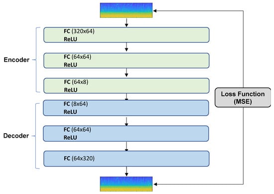
Figure 4. Architecture of the autoencoder–decoder neural network.

3.9. Neural Network Auto-Encoder-Decoder with LSTM

We implemented the autoencoder–decoder neural network with long-short-term memory (LSTM). The input features are the same as the baseline. The architecture has the LSTM layer and five more hidden layers (see Figure 5). The output of the LSTM layer is transferred to the autoencoder–decoder architecture, which is similar to the baseline architecture (Figure 6). The reconstruction loss function is MSE. Training was carried out for 50 epochs.

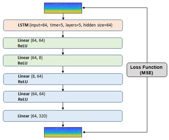
Figure 5. Front-end architecture of the convolutional autoencoder–decoder neural network with LSTM.

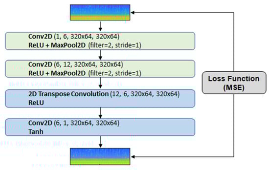
Figure 6. Back-end architecture of the convolutional autoencoder–decoder neural network.

3.10. Generative Adversarial Network

Another epoch of deep neural network architecture progress is a generative adversarial network (GAN) [52]. GAN is categorized as a generative model and is a framework for the estimation of generative models via an adversarial process in which two models, a discriminator and a generator, are trained simultaneously. The generator generates counterfeit images based on input noise, and the discriminator judges an input image as an original or the counterfeit one. The learning process in the original GAN framework is recognized as a Min–Max game where a generator and a discriminator are optimized with a value function $V\left(D,G\right)$ formulated as:

$$\underset{G}{min} \underset{D}{max}V\left(D, G\right)={\mathbb{E}}_{x\sim Pdata\left(x\right)}\left[log D\left(x\right)\right]+{\mathbb{E}}_{z\sim Pz\left(z\right)}\left[log\left(1-D\left(G\left(z\right)\right)\right)\right],$$

(28)

where the input noise variables are $Pz\left(z\right)$ and a mapping to the data space is represented as $G\left(z; \theta g\right)$. $D\left(x\right)$ represents the probability that $x$ came from the data rather than from the generator.

Here, we use a deep convolutional generative adversarial network for anomaly detection (AnoGAN). The architectural diagram of the network is presented in Figure 7.

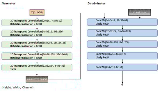
Figure 7. The architectural diagram of the Deep Convolutional Generative Adversarial Network for Anomaly Detection (AnoGAN).

3.11. Optimization

The Dice score coefficient (DSC) is a measure of overlap that is used to assess segmentation performance when a ground truth is available. We use the 2-class variant of DSC, which expresses the overlap between two classes A and B as:

$$DSC\left(A,B\right)=\frac{2\left|A\cap B\right|}{\left|A\right|+\left|B\right|}=\frac{2{{\displaystyle \sum }}_i^N{p}_i{g}_i}{{{\displaystyle \sum }}_i^N{p}_i^2+{{\displaystyle \sum }}_i^N{g}_i^2}.$$

(29)

3.12. Evaluation

The performance of anomaly detection is measured in the index of AUC which is a proven technique to evaluate binary classifier output quality used in communication engineering. In the evaluation process, the receiver operating characteristic (ROC) is plotted based on the false positive rate and true positive rate. The AUC is defined by the area of the curve. AUC has a range of 0 to 1. The higher AUC means the higher performance of binary classification, and 0.5 means that the discriminator judges the result randomly.

3.13. Development Environment

The machine specification was the following: 8 core Intel Core i9 CPU, Processor clock—2.4 GHz, No. of processors—1, and RAM—32 GB.

4. Experimental Analysis

4.1. Data Analysis

We conducted an initial data analysis on the dataset. Figure 8 shows the frequency and log-Mel spectrogram in the time domain figures of one of the.wav files of 6 dB SNR in the data set. A pump in normal condition operation contains high-intensity components in the frequency band of 50 Hz to 1 kHz. At the high-frequency band, randomly scattered components are observed, which are supposed to be environment noise. In contrast, a pump in anomalous condition showed a sudden change of sound, which implies pump trouble.

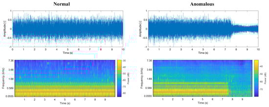
Figure 8. Example of the normalized amplitude of the pump ID: 06 at SNR 6 dB, frequency in the time domain (top row) and corresponding power spectrogram (bottom row) on normal condition (left column) and anomalous condition (right column).

Likewise, Figure 9 shows the frequency and power spectrogram in the time domain figures of one of the wav files of −6 dB SNR in the data set. In normal conditions, the frequency band in the range of 50 Hz to 1 kHz is corrupted, and its boundaries become unclear compared to those of the sound data with 6 dB SNR. The component in the broad domain of high frequency is highlighted because of its low SNR. The anomalous condition data, in this case, shows hunching every 2 s. The anomalous condition visualized in the time-frequency figure is ambiguous due to less −6 dB SNR, but the log-Mel spectrogram seems to have successfully highlighted the transition of sound components, which differ from the corresponding normal condition. Note that in the dataset the data are labeled only as normal and anomaly. No further description of this anomalous condition is given. Therefore, the anomalous condition needs to be detected as outlier data from the normal condition.

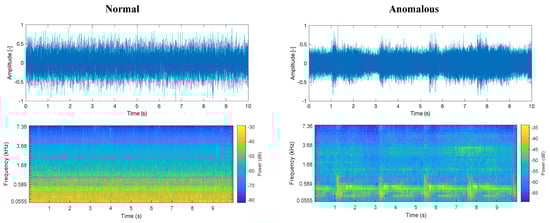
Figure 9. Example of normalized amplitude of the pump ID: 06 at −6 dB SNR, frequency in time domain (top row), and corresponding power spectrogram (bottom row) on normal condition (left column) and anomalous condition (right column).

4.2. Results of Dimensionality Reduction

The PCA of the signals was performed using the Python library scikit-Learn, version 0.22.1. Figure 10 shows graphs of the normal condition and anomalous condition data in a two-dimensional space reduced from the 64 × 313 features obtained by the log-Mel spectrogram using PCA. Pumps under normal conditions and anomalous conditions at 6 dB SNR are projected to different clusters in a two-dimensional space. In contrast, both normal condition and anomalous condition sound data are distributed onto similar regions, despite there seeming to be some clustering. The result implies the data of high SNR can be conducted in anomaly detection by conventional clustering methods such as k-mean clustering, but low SNR data need to be scrutinized by other methods which can embrace nonlinearity and reflect high-dimension information for detection.

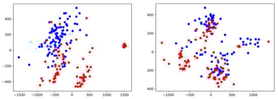
Figure 10. A pump ID: 06 operation sound data of 6 dB SNR (left) and −6 dB SNR (right). Projections of the 64 × 313 log-Mel spectrogram feature onto the 2D space by PCA. The symbols of blue and red represent the normal condition, and anomalous condition, respectively.

We also applied the stochastic neighborhood embedding method based on t distribution (t-SNE) method to reduce the dimension.

Figure 11 shows plots of the normal condition and anomalous condition data in two-dimensional space reduced from the 64 × 313 features obtained by the log-Mel spectrogram using t-SNE. t-SNE was done using the library scikit-Learn, version 0.22.1. The data at 6 dB SNR are clearer clustered than the plot obtained by PCA dimension reduction. The data at −6 dB SNR showed a cluster of anomaly condition data but most of the data were projected with a less clear boundary between normal condition and anomalous condition. t-SNE shows good anomaly detection performance for data with high-SNR but noisy data require other methods, such as PCA.

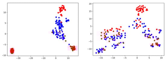
Figure 11. A pump ID06 operation sound data of 6 dB SNR (left) and −6 dB SNR (right). Projections of 64 × 313 dimensions log-Mel spectrogram features onto the estimated 2D space by t-SNE. The blue and red dots represent the normal condition and the anomalous condition, respectively.

The above results possess all the information of 10 (s) in one segment. Following the reproduction work, we also applied PCA and t-SNE dimensional reduction for 320-dimensional log-Mel spectrogram features. Figure 12 and Figure 13 show the data plots embedded in a 2D space by using PCA and t-SNE, respectively.

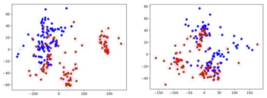
Figure 12. A pump ID: 06 operation sound data of 6 dB SNR 6 dB (left) and −6 dB SNR (right). Projections of the 320-dimension log-Mel spectrogram feature onto the 2D space by PCA. The blue and red symbols represent the normal condition and the anomalous condition, respectively.

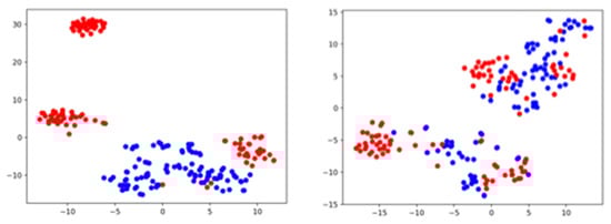
Figure 13. A pump ID06 operation sound data of 6 dB SNR (left) and −6 dB SNR (right). Projections of the 320-dimensional log-Mel spectrogram feature onto the estimated 2D space by t-SNE. The blue and red symbols represent the normal condition and the anomalous condition, respectively.

The 320-dimensional features represent a short period of 50/313 (s) out of 10 (s) as we discussed in session 3.1. The plot embedded in a 2-dimensional space using PCA showed a similar result as that of 313 × 64-dimensional features. On the contrary, the plot embedded into the 2D space using t-SNE showed a broader cluster compared to that of the 313 × 64-dimensional features for the data at 6 dB SNR but the cluster is still clearly separated between normal data and anomalous data. For the data at −6 dB SNR, the clustering of each condition seems effective in comparison to that of 313 × 64-dimensional features. It is implied that the impact of noise can be alleviated by focusing on a short period of time.

4.3. Results of the Autoencoder as the Baseline Model

As a baseline model, we used an autoencoder. The dataset provider presented the benchmark results with the model developed by using the Keras library, and we instead used PyTorch to double-check the feature engineering process and deep neural network models from the different approaches. The anomaly detection was performed for each segment by thresholding the reconstruction error averaged over 10 s. The network was trained using the Adam optimization technique for 50 epochs to minimize the loss function.

The results are given in Table 2 and Figure 14. Our result supported the benchmark result and the trend that noisy data exacerbate the failure detection performance. Moreover, in the majority of cases, we have managed to improve the SNR value over the benchmark values, especially when the benchmark value was low.

Table 2. Comparison of the SNR evaluated in the research with the benchmark SNR presented by the data set provider.

	Benchmark			Reproduced Result in Initial Data Analysis
Model ID	Input SNR			Input SNR
	6 dB	0 dB	−6 dB	6 dB	0 dB	−6 dB
ID00	0.84	0.65	0.58	0.84	0.67	0.70
ID02	0.45	0.46	0.52	0.64	0.43	0.50
ID04	0.99	0.95	0.93	0.99	0.99	0.91
ID06	0.94	0.76	0.61	0.91	0.86	0.59

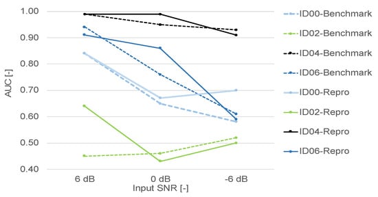
Figure 14. The benchmark AUC and the results of reproduction results.

4.4. Results of the One-Class Support Vector Machine as a Baseline Model

We conducted an unsupervised outlier detection method for the One-Class Support Vector Machine (OC-SVM). OC-SVM was tested on machine ID: 06 by using the library scikit-Learn, version 0.22.1.

The model was trained with normal condition data, excluding data for testing. The model was tested using the same sets of normal and abnormal conditions. The detection success rate is evaluated by the boundary determined by the trained model. Training and testing were conducted for both features of 64 × 313 and 320 dimensions.

The results are presented in Table 3. We observed that the OC-SVM determines the boundary of normal condition conservatively for both the feature dimensions, and this makes it difficult to screen anomalous conditions.

Table 3. Successfully selected rate of the normal and anomalous condition data of pump ID: 06 using OC-SVM.

Feature Dimensions	Performance Measure	Input SNR
		6 dB	0 dB	−6 dB
64 × 313	Accuracy of Normal Condition Data	0.91	0.93	0.96
	Accuracy of Anomalous Condition Data	0.78	0.40	0.58
320	Accuracy of Normal Condition Data	0.96	0.88	0.93
	Accuracy of Anomalous Condition Data	0.68	0.42	0.56

4.5. Results of the Autoencoder with LSTM

We have evaluated the autoencoder with LSTM architecture on the dataset. Training was carried out for 50 epochs. The reconstruction loss function used was MSE. Table 4 displays the results of the AUC. This architecture enhanced AUC for clean sound data (6 dB), while exacerbated AUC for noisy sound data (−6 dB). The result implies that if the SNR of sound is high enough, then LSTM which incorporates time-directional information works well. On the other hand, if the SNR of sound is low, LSTM cannot extract meaningful information from the noisy data.

Table 4. AUC evaluated by the autoencoder with LSTM on the pump ID: 06 at SNR of −6 dB.

Model ID	Input SNR
	6 dB	0 dB	−6 dB
ID06	0.9537	TBA	0.5941

4.6. Results of the Generative Adversarial Network for Anomaly Detection (ANOGAN)

We tested a deep-convolutional generative adversary network for anomaly detection (AnoGAN) on the data set to understand how convolution works in sound data and the overall trend overall the segment time interval of 10 (sec). The input feature is prepared by converting the log-Mel spectrogram into a jpeg figure with a librosa built-in function. Pump ID: 06 is used for the testing at each input SNR value. Therefore, the jpeg figure contains log-Mel spectrogram information for 10 (sec). The converted jpeg figures have a pixel size of 640 × 480 and RGB as shown in Figure 15. Figures are converted and resized to 64 × 64 pixels and then normalized to the range of 0 to 1 to fit the GAN. The model is developed with Python PyTorch library. Training was carried out for 50 epochs. The Logistic Loss function was used to measure reconstruction loss.

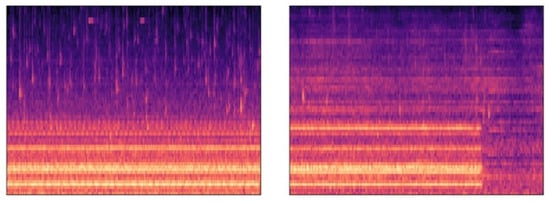
Figure 15. Example of a log-Mel spectrogram of pump ID: 06 at 6 dB SNR of normal condition (left) and anomalous condition (right) in image format.

Table 5 shows the result of the AnoGAN. The AUC is lower than 0.5 and indicates that AnoGAN does not work in the dataset. One of the potential reasons is that compressing the jpeg file from 640 × 480 to 64 × 64 lost data in a short time interval. The other possible reason is that the overall 10 (s) data are too large to depict operating information.

Table 5. AUC evaluated by ANOGAN on the pump ID: 06.

Model ID	Input SNR
	6 dB	6 dB	−6 dB
ID06	0.44	0.46	0.41

Table 6 shows the results of AUC for the various preprocessing methods and loss functions in the autoencoder–decoder neural network on the sound data of the pump ID: 06 at SNR of −6 dB. The proposed schematics using UKF and MSE with the L2 regularization term showed an improvement of AUC for the noisy pump data of pump (ID: 06 at SNR −6 dB) from 0.7633 (baseline) to 0.7907 (using MSE with L2 regularization). The results implied that the data preprocessing by the adaptive filters has impact on the performance of anomaly detection using a neural network; hence, the loss function should be designed in accordance with the design of the applied adaptive filters.

Table 6. Summary of AUC for the various preprocessing methods and loss functions in the autoencoder–decoder neural network on the sound data of the pump ID: 06 at SNR of −6 dB. KF—Kalman Filter. UKF—Unscented Kalman Filter. MSE—mean square error.

Pre-Processing	Loss Function	AUC
Raw (unprocessed)	MSE	0.7633 ± 0.0239 (Baseline)
	MSE MSE with L2 Regularization	0.7644 ± 0.0165 0.7909 ± 0.0192
KF	MSE	0.7764 ± 0.0250
	MSE with L2 Regularization	0.7898 ± 0.0200
UKF	MSE	0.7644 ± 0.0165
	MSE with L2 Regularization	0.7909 ± 0.0192

4.7. Analysis of Misclassifications

Among the normal-condition dataset, we successfully detected normal condition with a minimum reconstruction error of 2848, 00000659.wav. On the other hand, we mistakenly detected as anomalous condition with the highest reconstruction error of 6214, 00000038.wav. These sound data are shown in Figure 16. The data from 00000659.wav showed a momentary loud sound at 4 s elapsed.

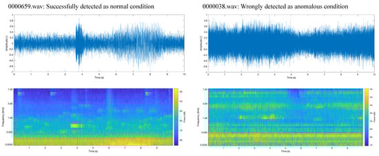
Figure 16. Examples of spectrum images of the normal condition data for pump ID 06 at SNR −6 dB.

Likewise, among the anomalous-condition dataset, successfully detected anomalous condition with the highest reconstruction error of 6736 is 00000077.wav. The incorrectly detected anomalous condition with the lowest reconstruction error of 2738 was 00000005.wav. These sound data are visually shown in Figure 17. In the case of 00000077.wav, somewhat periodic peaks each 2 (s) can be observed. This periodic anomalous information enabled the autoencoder to detect the anomaly. In contrast, the case of 00000005.wav shows that the signal information is covered with background noise.

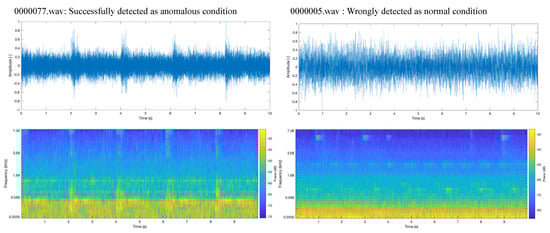
Figure 17. Examples of spectrum images of the anomalous condition data for pump ID 06 at SNR −6 dB.

5. Discussion and Comparison with Similar Works

Purohit et al. [58] presented the benchmark performance of unsupervised anomaly detection for the dataset using the autoencoder-based model, assuming that anomalous data cannot be reconstructed from a compressed representation layer in the model trained by normal condition data only. In the benchmark experiment setup, the Log-Mel spectrogram is considered as an input feature. The spectrogram is based on the conditions: frame size 1024; hop size 512, and Mel filters 64. This generates 313 frames in time and 64 cells for the frequency domain, where the total features are 313 × 64 in one segment of 10-s sound data. The five frames in time are combined to initiate a 320-dimension input feature vector. Therefore, an input feature represents 50/313 (s) time domain. The rest of the normal segments is a test dataset.

The training of the model is conducted using normal condition sound data, and the test is conducted using anomalous condition data and normal condition sound data, excluding the data used for training. The performance of anomaly detection is evaluated by the Curve (AUC). They concluded that nonstationary machinery, such as slide rails and valves, and noisy data, that is, low input SNR in the context, is the key challenge in anomaly detection of this machinery. The impact of noise on performance is implied in Table 7. As an instance of stationary machines, the pumps of ID 00 with 6 dB input SNR showed an AUC of 0.84, while −6 dB input SNR shows an AUC of 0.58. The machine ID: 02 showed different behavior, but a reason was not stated in the literature.

Table 7. Comparison of the AUC values of pumps with ID: 00, 02, 04, and 06 at the input SNR of 6 dB, 0 dB, and −6 dB.

Model ID	Input SNR [36]		Input SNR (This Paper)
	6 dB	0 dB	−6 dB	6 dB	0 dB	−6 dB
ID00	0.84	0.65	0.58	0.8212	0.6792	0.6741
ID02	0.45	0.46	0.52	0.5938	0.5576	0.5293
ID04	0.99	0.95	0.93	0.9979	0.9753	0.9226
ID06	0.94	0.76	0.61	0.9281	0.7854	0.6518

6. Conclusions and Future Work

In this study, we proposed an anomaly detection system for the analysis of real-life industrial machinery failure sounds. To our knowledge, few studies are focusing on the relationship between the data pre-processing and cost functions in neural network architecture. The proposed system consists of the preprocessing component, which applies the Unscented Kalman Filter (UKF) for state estimation, and of the anomaly detection component, which has an autoencoder–decoder neural network with Tikhonov regularization (diagonal loading).

The results implied that the data preprocessing by the adaptive filters impacts the performance of anomaly detection using a neural network; hence, the loss function should be designed in accordance with the design of the applied adaptive filters.

The autoencoder–decoder model showed superior performance compared to other classification techniques in noisy data analysis.

The results of this study suggest what acoustic detection of failures could be used for Predictive Maintenance [61] of industrial machinery in the context of Industry 4.0. The incorporation of acoustic new sensor technologies combined with deep learning methods can be used to avoid premature replacement of equipment, saving maintenance costs, improving machining process safety, increasing availability of equipment, and maintaining the acceptable levels of performance [2]. The predictive maintenance system in smart factories based on acoustic failure pattern recognition can serve as an early warning system for managers, especially in high-risk industrial businesses. The ability to detect weak signals with potentially substantial strategic implications is a welcome benefit of process automation in the corporate world. Their key benefit is real-time management and planning, which helps to cut down on the costs of production downtime [62].

Future work will focus on modeling deep neural networks reflecting local neighborhood relationships, and on feature engineering for noise reduction in the low-SNR sound dataset. We will explore the deep convolutional neural network approach to short-time data instead of applying overall 10-second data, and modification to loss function to reflect neighborhood relationship in manifold learning of the autoencoder (metric learning approach). Furthermore, we aim to investigate methods applicable to robust speaker identification, especially those oriented at noisy environments, which might further help improving the quality of acoustic fault detection, within industrial environments.

References

- Chandola, V.; Banerjee, A.; Kumar, V. Anomaly detection: A survey. ACM Comput. Surv. 2009, 41, 1–58. [Google Scholar] [CrossRef]
- Çınar, Z.M.; Nuhu, A.A.; Zeeshan, Q.; Korhan, O.; Asmael, M.; Safaei, B. Machine learning in predictive maintenance towards sustainable smart manufacturing in industry 4.0. Sustainability 2020, 12, 8211. [Google Scholar] [CrossRef]
- An, Q.; Tao, Z.; Xu, X.; El Mansori, M.; Chen, M. A data-driven model for milling tool remaining useful life prediction with convolutional and stacked LSTM network. Measurement 2020, 15, 107461. [Google Scholar] [CrossRef]
- Lv, Y.; Liu, Y.; Jing, W.; Woźniak, M.; Damaševičius, R.; Scherer, R.; Wei, W. Quality control of the continuous hot pressing process of medium density fiberboard using fuzzy failure mode and effects analysis. Appl. Sci. 2020, 10, 4627. [Google Scholar] [CrossRef]
- Kawaguchi, Y.; Endo, T. How can we detect anomalies from subsampled audio signals? In Proceedings of the 2017 IEEE International Workshop on Machine Learning for Signal Processing, Tokyo, Japan, 25–28 September 2017. [Google Scholar] [CrossRef]
- Kawaguchi, Y. Anomaly detection based on feature reconstruction from subsampled audio signals. In Proceedings of the 26th European Signal Processing Conference (EUSIPCO), Rome, Italy, 3–8 September 2018; pp. 2538–2542. [Google Scholar]
- Marchie, E.; Vesperini, F.; Eyben, F.; Squartini, S.; Schuller, B. A novel approach for automatic acoustic novelty detection using a denoising autoencoder with bidirectional LSTM neural networks. In Proceedings of the International Conference on Acoustics, Speech, and Signal Processing (ICASSP), South Brisbane, Australia, 19–24 April 2015; pp. 1996–2000. [Google Scholar]
- Koizumi, Y.; Saito, S.; Uematsu, H.; Harada, N. Optimizing acoustic feature extractor for anomalous sound detection based on Neyman-Pearson lemma. In Proceedings of the 25th European Signal Processing Conference (EUSIPCO), Kos, Greece, 28 August–2 September 2017; pp. 698–702. [Google Scholar]
- Licitra, G.; Fredianelli, L.; Petri, D.; Vigotti, M.A. Annoyance evaluation due to overall railway noise and vibration in Pisa urban areas. Sci. Total Environ. 2016, 568, 1315–1325. [Google Scholar] [CrossRef]
- Miedema, H.M.E.; Oudshoorn, C.G.M. Annoyance from transportation noise: Relationships with exposure metrics DNL and DENL and their confidence intervals. Environ. Health Perspect. 2001, 109, 409–416. [Google Scholar] [CrossRef]
- Vukić, L.; Fredianelli, L.; Plazibat, V. Seafarers’ Perception and attitudes towards noise emission on board ships. Int. J. Environ. Res. Public Health 2021, 18, 6671. [Google Scholar] [CrossRef]
- Rossi, L.; Prato, A.; Lesina, L.; Schiavi, A. Effects of low-frequency noise on human cognitive performances in laboratory. Build. Acoust. 2018, 25, 17–33. [Google Scholar] [CrossRef]
- Minichilli, F.; Gorini, F.; Ascari, E.; Bianchi, F.; Coi, A.; Fredianelli, L.; Licitra, G.; Manzoli, F.; Mezzasalma, L.; Cori, L. Annoyance judgment and measurements of environmental noise: A focus on Italian secondary schools. Int. J. Environ. Res. Public Health 2018, 15, 208. [Google Scholar] [CrossRef] [Green Version]
- Erickson, L.C.; Newman, R.S. Influences of background noise on infants and children. Curr. Dir. Psychol. Sci. 2017, 26, 451–457. [Google Scholar] [CrossRef]
- Dratva, J.; Phuleria, H.C.; Foraster, M.; Gaspoz, J.M.; Keidel, D.; Künzli, N.; Liu, L.J.; Pons, M.; Zemp, E.; Gerbase, M.W.; et al. Transportation noise and blood pressure in a population-based sample of adults. Environ. Health Perspect. 2012, 120, 50–55. [Google Scholar] [CrossRef]
- Petri, D.; Licitra, G.; Vigotti, M.A.; Fredianelli, L. Effects of exposure to road, railway, airport and recreational noise on blood pressure and hypertension. Int. J. Environ. Res. Public Health 2021, 18, 9145. [Google Scholar] [CrossRef]
- Babisch, W.; Beule, B.; Schust, M.; Kersten, N.; Ising, H. Traffic noise and risk of myocardial infarction. Epidemiology 2005, 16, 33–40. [Google Scholar] [CrossRef]
- Ajitha, P.; Chandra, E. Survey on outliers detection in distributed data mining for big data. J. Basic Appl. Sci. Res. 2015, 5, 31–38. [Google Scholar]
- Calabrese, F.; Regattieri, A.; Bortolini, M.; Gamberi, M.; Pilati, F. Predictive maintenance: A novel framework for a data-driven, semi-supervised, and partially online prognostic health management application in industries. Appl. Sci. 2021, 11, 3380. [Google Scholar] [CrossRef]
- Tanuska, P.; Spendla, L.; Kebisek, M.; Duris, R.; Stremy, M. Smart anomaly detection and prediction for assembly process maintenance in compliance with industry 4.0. Sensors 2021, 21, 2376. [Google Scholar] [CrossRef]
- Peng, C.-Y.; Raihany, U.; Kuo, S.-W.; Chen, Y.-Z. Sound detection monitoring tool in CNC milling sounds by K-means clustering algorithm. Sensors 2021, 21, 4288. [Google Scholar] [CrossRef]
- Kim, D.; Lee, S.; Kim, D. An applicable predictive maintenance framework for the absence of run-to-failure data. Appl. Sci. 2021, 11, 5180. [Google Scholar] [CrossRef]
- Skoczylas, A.; Stefaniak, P.; Anufriiev, S.; Jachnik, B. Belt conveyors rollers diagnostics based on acoustic signal collected using autonomous legged inspection robot. Appl. Sci. 2021, 11, 2299. [Google Scholar] [CrossRef]
- Ho, S.K.; Nedunuri, H.C.; Balachandran, W.; Kanfoud, J.; Gan, T.-H. Monitoring of industrial machine using a novel blind feature extraction approach. Appl. Sci. 2021, 11, 5792. [Google Scholar] [CrossRef]
- Mey, O.; Schneider, A.; Enge-Rosenblatt, O.; Mayer, D.; Schmidt, C.; Klein, S.; Herrmann, H.-G. Condition monitoring of drive trains by data fusion of acoustic emission and vibration sensors. Processes 2021, 9, 1108. [Google Scholar] [CrossRef]
- Serradilla, O.; Zugasti, E.; Ramirez de Okariz, J.; Rodriguez, J.; Zurutuza, U. Adaptable and explainable predictive maintenance: Semi-supervised deep learning for anomaly detection and diagnosis in press machine data. Appl. Sci. 2021, 11, 7376. [Google Scholar] [CrossRef]
- Wei, Y.; Li, Y.; Xu, M.; Huang, W. A review of early fault diagnosis approaches and their applications in rotating machinery. Entropy 2019, 21, 409. [Google Scholar] [CrossRef] [PubMed] [Green Version]
- Saufi, S.R.; Ahmad, Z.A.B.; Leong, M.S.; Lim, M.H. Challenges and opportunities of deep Learning models for machinery fault detection and diagnosis: A Review. IEEE Access 2019, 7, 122644. [Google Scholar] [CrossRef]
- Wang, D.; Brown, G.J. Computational Auditory Scene Analysis: Principles, Algorithms, and Applications; Wiley/IEEE Press: Piscataway, NJ, USA, 2006. [Google Scholar]
- Williamson, D.S.; Wang, D. Speech dereverberation and denoising using complex ratio masks. In Proceedings of the 2017 IEEE International Conference on Acoustics, Speech and Signal Processing (ICASSP), New Orleans, LA, USA, 5–9 March 2017; pp. 5590–5594. [Google Scholar] [CrossRef]
- Ayhan, B.; Kwan, C. Robust speaker identification algorithms and results in noisy environments; Lecture Notes in Computer Science. In Proceedings of the Advances in Neural Networks—ISNN 2018, Minsk, Belarus, 25–28 June; Huang, T., Lv, J., Sun, C., Tuzikov, A., Eds.; Springer: Cham, Switzerland; Volume 10878, pp. 443–450.
- Zhang, M.; Guo, J.; Li, X.; Jin, R. Data-driven anomaly detection approach for time-series streaming data. Sensors 2020, 20, 5646. [Google Scholar] [CrossRef] [PubMed]
- Pittino, F.; Puggl, M.; Moldaschl, T.; Hirschl, C. Automatic anomaly detection on in-production manufacturing machines using statistical learning methods. Sensors 2020, 20, 2344. [Google Scholar] [CrossRef] [PubMed] [Green Version]
- Hyvarinen, A.; Karhunen, H.; Oja, E. Independent Component Analysis; Wiley-Interscience: Hoboken, NJ, USA, 2001. [Google Scholar]
- Ikeda, S.; Toyama, K. Independent component analysis for noisy data—MEG data analysis. Neural Netw. 2000, 13, 1063–1074. [Google Scholar] [CrossRef]
- Koganeyama, M. An effective evaluation function for ICA to separate train noise from telluric current data. In Proceedings of the 4th International Symposium on Independent Component Analysis and Blind Signal Separation (ICA2003), Nara, Japan, 1–4 April 2003; pp. 837–842. [Google Scholar]
- Damaševičius, R.; Napoli, C.; Sidekerskienė, T.; Woźniak, M. IMF mode demixing in EMD for jitter analysis. J. Comput. Sci. 2017, 22, 240–252. [Google Scholar] [CrossRef]
- Kebabsa, T.; Ouelaa, N.; Djebala, A. Experimental vibratory analysis of a fan motor in industrial environment. Int. J. Adv. Manuf. Technol. 2018, 98, 2439–2447. [Google Scholar] [CrossRef]
- Garnier, J.; Solna, K. Applications of random matrix theory for sensor array imaging with measurement noise. Random Matrices 2014, 65, 223–245. [Google Scholar]
- Gu, X.; Akoglu, L.; Rinaldo, A. Statistical analysis of nearest neighbor methods for anomaly detection. In Proceedings of the 33rd Conference on Neural Information Processing Systems (NeurIPS 2019), Vancouver, BC, Canada, 8–14 December 2019; pp. 10921–10931. [Google Scholar]
- Scholkopf, B.; Williamson, R.; Smola, A.; Shawe-Taylor, J.; Platt, J. Support vector method for novelty detection. In Proceedings of the 12th International Conference on Neural Information Processing Systems (NIPS′99), Denver, CO, USA, 29 November–4 December 1999; pp. 582–588. [Google Scholar]
- Hsu, J.; Wang, Y.; Lin, K.; Chen, M.; Hsu, J.H. Wind turbine fault diagnosis and predictive maintenance through statistical process control and machine learning. IEEE Access 2020, 8, 23427–23439. [Google Scholar] [CrossRef]
- Toma, R.N.; Prosvirin, A.E.; Kim, J. Bearing fault diagnosis of induction motors using a genetic algorithm and machine learning classifiers. Sensors 2020, 20, 1884. [Google Scholar] [CrossRef] [Green Version]
- Sakurada, M.; Yairi, T. Anomaly detection using autoencoders with nonlinear dimensionality reduction. In Proceedings of the MLSDA 2014 2nd Workshop on Machine Learning for Sensory Data Analysis, Gold Coast, Australia, 2 December 2014; pp. 4–11. [Google Scholar]
- Ruff, L.; Vandermeulen, R.; Goernitz, N.; Deecke, L.; Siddiqui, S.A.; Binder, A.; Müller, E.; Kloft, M. Deep one-class classification. In Proceedings of the 35th International Conference on Machine Learning, Stockholm, Sweden, 10–15 July 2018; pp. 4393–4402. [Google Scholar]
- Luwei, K.C.; Yunusa-Kaltungo, A.; Sha’aban, Y.A. Integrated fault detection framework for classifying rotating machine faults using frequency domain data fusion and artificial neural networks. Machines 2018, 6, 59. [Google Scholar] [CrossRef] [Green Version]
- Zhao, H.; Liu, H.; Hu, W.; Yan, X. Anomaly detection and fault analysis of wind turbine components based on deep learning network. Renew. Energy 2018, 127, 825–834. [Google Scholar] [CrossRef]
- Dongo, Y.; Il, D.Y. Residual error based anomaly detection using auto-encoder in SMD machine sound. Sensors 2018, 18, 5. [Google Scholar]
- Cheng, Y.; Zhu, H.; Wu, J.; Shao, X. Machine health monitoring using adaptive kernel spectral clustering and deep long short-term memory recurrent neural networks. IEEE Trans. Ind. Inform. 2019, 15, 987–997. [Google Scholar] [CrossRef]
- Li, M.; Wang, S.; Fang, S.; Zhao, J. Anomaly detection of wind turbines based on deep small-world neural network. Appl. Sci. 2020, 10, 1243. [Google Scholar] [CrossRef] [Green Version]
- Chalapathy, R.; Chawla, S. Deep learning for anomaly detection: A Survey. arXiv 2019, arXiv:1901.03407v2. [Google Scholar]
- Goodfellow, I.J.; Pouget-Abadie, J.; Mirza, M.; Xu, B.; Warde-Farley, D.; Ozair, S.; Courville, A.; Bengio, Y. Generative adversarial nets. Adv. Neural Inform. Process. Syst. 2014, 27, 1–9. [Google Scholar]
- Schlegl, T.; Seeböck, P.; Waldstein, S.M.; Schmidt-Erfurth, U.; Langs, G. Unsupervised anomaly detection with generative adversarial networks to guide maker discovery. In Proceedings of the Information Processing in Medical Imaging 2017, Boone, NC, USA, 25–30 June 2017; pp. 146–157. [Google Scholar]
- Schlegl, T.; Seeböck, P.; Waldstein, S.M.; Langs, G.; Schmidt-Erfurth, U. f-AnoGAN: Fast unsupervised anomaly detection with generative adversarial networks. Med. Image Anal. 2019, 54, 30–44. [Google Scholar] [CrossRef]
- Wu, J.; Zhao, Z.; Sun, C.; Yan, R.; Chen, X. Fault-attention generative probabilistic adversarial autoencoder for machine anomaly detection. IEEE Trans. Ind. Inform. 2020, 16, 7479–7488. [Google Scholar] [CrossRef]
- Zhang, G.; Xiao, H.; Jiang, J.; Liu, Q.; Liu, Y.; Wang, L. A Multi-index generative adversarial network for tool wear detection with imbalanced data. Complexity 2020, 2020, 5831632. [Google Scholar] [CrossRef]
- Zenodo Website. MIMII Dataset: Sound Dataset for Malfunctioning Industrial Machine Investigation and Inspection. Available online: https://zenodo.org/record/3384388 (accessed on 28 December 2019).
- Purohit, H.; Tanabe, R.; Ichige, K.; Endo, T.; Nikaido, Y.; Suefusa, K.; Kawaguchi, Y. MIMII dataset: Sound dataset for malfunctioning industrial machine investigation and inspection. In Proceedings of the 4th Workshop on Detection and Classification of Acoustic Scenes and Events (DCASE), New York, NY, USA, 25–26 October 2019; pp. 209–213. [Google Scholar]
- Van der Maaten, L.; Hinton, G. Visualizing data using t-SNE. J. Mach. Learn. Res. 2008, 9, 2579–2605. [Google Scholar]
- Breunig, M.M.; Kriegel, H.P.; Ng, R.T.; Sander, J. LOF: Identifying density-based local outliers. In Proceedings of the International Conference on Management of Data, Dallas, TX, USA, 15–18 May 2000; pp. 93–104. [Google Scholar]
- Cardoso, D.; Ferreira, L. Application of predictive maintenance concepts using artificial intelligence tools. Appl. Sci. 2021, 11, 18. [Google Scholar] [CrossRef]
- Pech, M.; Vrchota, J.; Bednář, J. Predictive maintenance and intelligent sensors in smart factory: Review. Sensors 2021, 21, 1470. [Google Scholar] [CrossRef]
Publisher’s Note: MDPI stays neutral with regard to jurisdictional claims in published maps and institutional affiliations. |
© 2021 by the authors. Licensee MDPI, Basel, Switzerland. This article is an open access article distributed under the terms and conditions of the Creative Commons Attribution (CC BY) license (https://creativecommons.org/licenses/by/4.0/).