A Hybrid-Driven Optimization Framework for Fixed-Wing UAV Maneuvering Flight Planning

Abstract

Performing autonomous maneuvering flight planning and optimization remains a challenge for unmanned aerial vehicles (UAVs), especially for fixed-wing UAVs due to its high maneuverability and model complexity. A novel hybrid-driven fixed-wing UAV maneuver optimization framework, inspired by apprenticeship learning and nonlinear programing approaches, is proposed in this paper. The work consists of two main aspects: (1) Identifying the model parameters for a certain fixed-wing UAV based on the demonstrated flight data performed by human pilot. Then, the features of the maneuvers can be described by the positional/attitude/compound key-frames. Eventually, each of the maneuvers can be decomposed into several motion primitives. (2) Formulating the maneuver planning issue into a minimum-time optimization problem, a novel nonlinear programming algorithm was developed, which was unnecessary to determine the exact time for the UAV to pass by the key-frames. The simulation results illustrate the effectiveness of the proposed framework in several scenarios, as both the preservation of geometric features and the minimization of maneuver times were ensured.

1. Introduction

Recent times have witnessed a wide range of applications for unmanned aerial vehicles (UAVs) including the commercial, military, and research fields [1,2,3,4,5]. Most of the autonomous UAV flight missions are limited to cruise on a predefined path with steady flight states. However, in some scenarios, such as dog fights and high-speed obstacle avoidance, UAVs are required to perform fast and agile maneuver flights. During maneuvers, drastic changes in position and attitude will hinder UAVs from maintaining trim conditions. Therefore, developing maneuvering flight techniques is of great importance, and the current research mainly focuses on the quadrotor UAV [6,7,8,9]. It must be noted that fixed-wing UAVs have longer endurance and a larger payload capacity compared to those of the quadrotors. Yet the maneuvers of fixed-wing UAVs have not been thoroughly studied due to the fact of its sophisticated movement features [10]. Meanwhile, it is harder to conduct real flight tests also.

The research on autonomous maneuverable flight is assumed to be hierarchical including several topics such as maneuver decision-making, maneuver planning, and tracking control [11]. The planner first decides the category of the maneuver, then generates a specific trajectory for the tracking control. Among them, maneuver planning is essential for the maneuverability of UAVs. In this article, we were mainly concerned with maneuver planning issues. When validating the complex maneuver representation approaches, appropriate maneuver generation algorithms are also considered.

Generally, state-of-the-art maneuver generation algorithms incorporate data-driven [12] and model-driven approaches. One category of maneuver generation algorithms that have been successfully utilized in UAV maneuver generation is learning from demonstration [13]. By collecting the flight data taught by experts with a high-level planning layer, imitating learning methods can be applied to extract the maneuver features [14]. The resulting algorithm is practically capable of reproducing and generalizing the learned motions to some extent. However, due to the limitations of viewing distance, communication delay, and external disturbances, such as wind gusts, it is hard for the pilot to perform their flight skills optimally [11]. Therefore, optimality is essential in the learning procedure and few of the data-driven algorithms in the recent literature take the optimization into consideration.

In the robotic literature, model-driven planning has been widely studied and the typical approaches include polynomial interpolation, Dubins curve [10,15,16]. For some special scenarios, it is essential to plan the position and attitude trajectories simultaneously. Therefore, many researchers have also made explorations in SE(3) space [17,18,19]. Most of the methods are based on the differential flatness principle which can greatly simplify the calculation complexity. However, for fixed-wing UAV flight maneuvers, it has to be stressed that those approaches did not take the complicated physical models with complex aerodynamic features into consideration. Therefore, the non-differential flatness property of fixed-wing UAV [20] hinders the application of the aforementioned methods. Solving the optimal control problems is also an effective maneuver planning method and has attracted growing attention. In particular, both the direct optimization method and indirect optimization methods have been applied in UAV flights in recent years [21,22,23]. Through taking the physical model into consideration, dynamical feasibility is ensured. Furthermore, by combing various cost items, optimal maneuvers can be solved for different scenarios [24]. However, for complex maneuvers, it is always hard to model the optimization problem, which has a great impact on the calculation efficiency and trajectory quality. In visual tracking [25,26], maneuvering is also required, vision-and-language navigation [27,28,29,30] provides another novel perspective. This method combines vision, language, and action which can turn relatively general natural-language instructions into robot agent actions. It is generally used in indoor complex environments and also has certain lightening significance for fixed-wing tracking of dynamic targets or maneuvering in complex outdoor environments.

For the representation of complex maneuvers, one recent algorithm that has been successfully proposed is the idea of key-frames [31], which selects several specific points in 3D space as the key-frames and various tasks can be accomplished. In [32], both the position and yaw angle are taken into account in the key-frame and the minimum snap trajectory is generated using polynomials. Furthermore, the author formulates the trajectory optimization problem as a quadratic programming issue and then enables the quadrotors to pass through multiple circular hoops quickly. Ref. [33] emphasizes the Bang-Bang characteristics of the minimum time trajectory and compares the existing time-optimal approaches, and through analysis, it is concluded that the polynomial method can only obtain non-optimal trajectories. On this basis, Foehn proposes complementary constraints [34] and solved both the time allocation and time-optimal trajectory planning problem elaborately. Through comparison and verification, it can be concluded that the trajectory designed by the algorithm is faster than that of professional pilots. For fixed-wing, a model is required, which can be obtained by identifying methods [35]. In addition, it focuses on the minimum time problem through setting a series of waypoints and utilizing the flight corridors and B-spline curves. Using numerical optimization methods to solve non-convex problems and cleverly designed initial guesses, the optimal trajectory is obtained. As for the fixed-wing UAV maneuver, it is hard to extract the trajectory features merely from position information. It is necessary to comprehensively consider the position and attitude features and design the corresponding key-frames for various maneuvers. Motion primitives also have a satisfactory effect on the decomposition of complex maneuvers [36]. Mueller and D’Andrea [15] proposed a framework for the efficient calculation of motion primitives. McGill University has presented a series of representative works based on the idea of motion primitives and maneuver optimization [37,38,39]. Dynamic motion primitives (DMPs) is a typical primitive which has been successfully utilized in the design of car driving motion libraries [40]. Inspired by the former works, we studied the dual quaternion-based dynamic motion primitives (DQ-DMPs) [41], which have the ability to learn and generalize maneuvers in SE(3) space. Nevertheless, it is hard for the dynamic motion primitive algorithm to ensure the kinodynamic feasibility.

Inspired by the above discussion, we propose a data-model-driven framework, which is shown in Figure 1, for fixed-wing UAV maneuvering optimization. The framework is based on a global model identified by teaching data, and uses an optimization method based on positional, attitude, and compound key-frames. Through numerical optimization, the time-optimal maneuver is finally obtained. Through comparison, the actions generated by this algorithm take less time than professional pilots. In complex actions, different primitives can be flexibly concatenated, which simplifies the generation of complex actions. The main contribution of this paper is listed as follows:

(1)

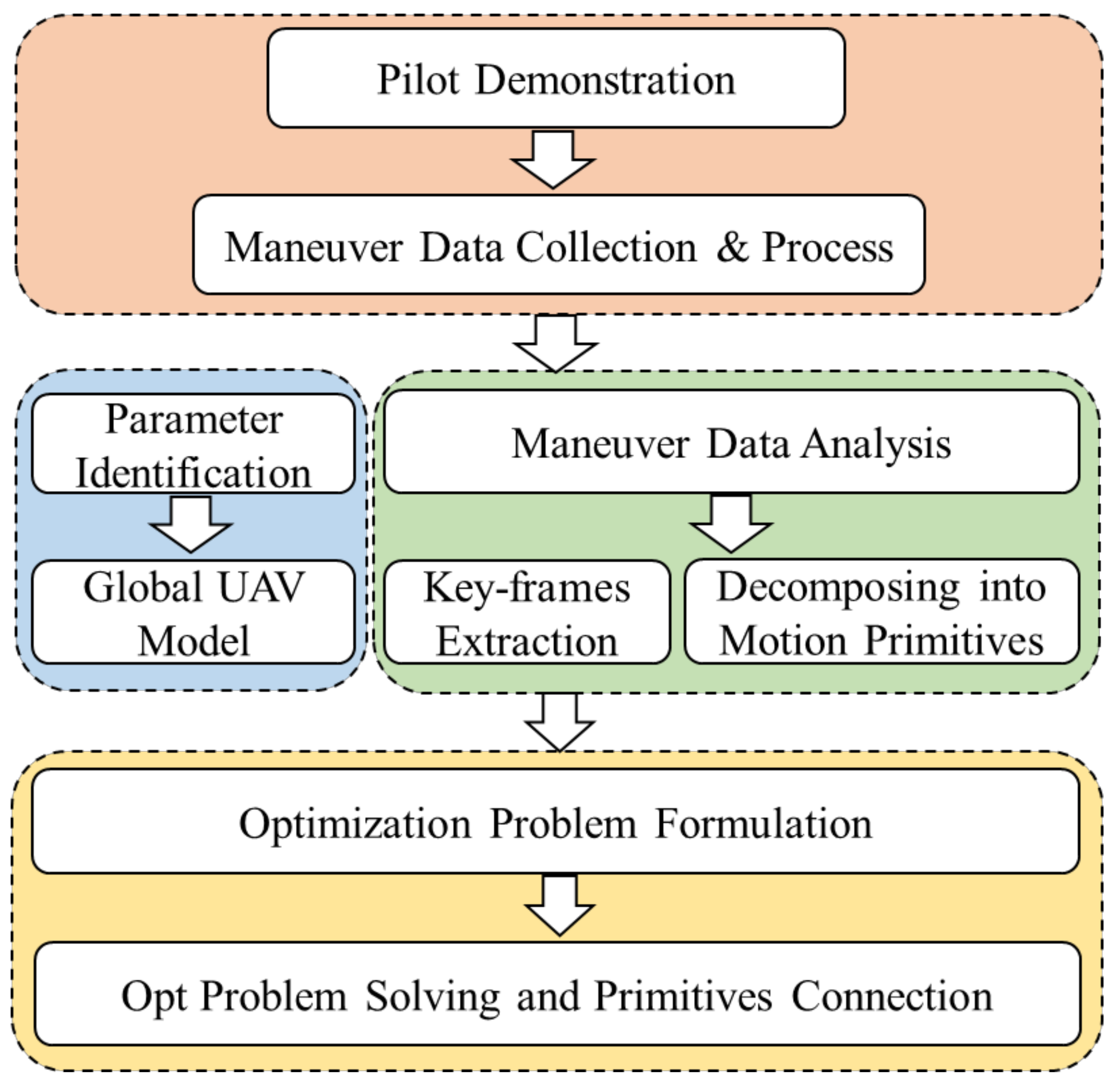
We proposed a novel data-driven approach for model identification and key-frames extraction using the learning from demonstration principles. Then, complex maneuvers are decomposed into multiple motion primitives;

(2)

Based on the motion primitives, the optimal maneuver generation issue is formulated into a time-optimal problem considering key-frames which the UAV must pass by. The connection method of different primitives was also considered in this paper for practicability;

(3)

The proposed framework was verified thoroughly in simulation experiments, and it was possible to deduce that this framework is applicable for flight maneuvers in reality.

In the next section, we discuss the basic knowledge. Section 3 and Section 4 introduce data collection and acrobatic maneuver optimization, respectively. The experimental results are introduced in Section 5, and the conclusion in Section 6.

2. Preliminaries

2.1. Global Fixed-Wing Model

The aircraft model plays an important role in our algorithm framework. In order to obtain feasible maneuvers, we need to establish a relatively accurate rigid-body model. Due to the singular problem of Euler angle during the big maneuver, this paper adopted the quaternion model [42] to calculate:

$$\begin{array}{l}{\dot{p}}^i=R\left(q\right)\cdot v^b\\ \dot{q}=\frac{1}{2}\left[{\omega }^b\otimes \right]q\\ {\dot{v}}^b=m^{-1}\left(F+T\right)-{\omega }^b\times v^b\\ {\dot{\omega }}^b=J^{-1}\left(\mathsf{\tau }-{\omega }^b\times J{\omega }^b\right)\end{array}$$

(1)

For translational kinematics equation, the $p^i=[x,y,z]\in {ℝ}^3$ is the position of the inertial coordinate system, and $v^b=[u,v,w]$ is the speed of the body coordinate system. The two state quantities are connected by a conversion matrix, which is composed of $q$, where $q={[q_0,q_1,q_2,q_3]}^T\in SO\left(3\right)$ is a unit quaternion given $‖q‖=1$. The rotation matrix is:

$$R\left(q\right)=\left[\begin{array}{ccc}\left(q_0{}^2+q_1{}^2-q_2{}^2-q_3{}^2\right)& 2\left(q_1{q}_2-q_0{q}_3\right)& 2\left(q_1{q}_3+q_0{q}_2\right)\\ 2\left(q_1{q}_2+q_0{q}_3\right)& \left(q_0{}^2-q_1{}^2+q_2{}^2-q_3{}^2\right)& 2\left(q_2{q}_3-q_0{q}_1\right)\\ 2\left(q_1{q}_3-q_0{q}_2\right)& 2\left(q_2{q}_3+q_0{q}_1\right)& \left(q_0{}^2-q_1{}^2-q_2{}^2+q_3{}^2\right)\end{array}\right]$$

(2)

In rotational kinematics equation, ${\omega }^b=[p^b,q^b,r^b]$ where $p^b,q^b,r^b$ is angular rate, we can write:

$$\left[{\omega }^b\otimes \right]=\left[\begin{array}{cccc}0& -p^b& -q^b& -r^b\\ p^b& 0& r^b& -q^b\\ q^b& -r^b& 0& p^b\\ r^b& q^b& -p^b& 0\end{array}\right]$$

(3)

In the translational dynamic equation, $T=[F_T,0,0]$, $F_T$ is the thrust, and

$$F=F_A+F_g=\left[\begin{array}{l}{F}_x+2\left(q_1{q}_3-q_0{q}_2\right)mg\\ F_y+2\left(q_2{q}_3+q_0{q}_1\right)mg\\ F_z+2\left(q_0{}^2-q_1{}^2-q_2{}^2+q_3{}^2\right)mg\end{array}\right]$$

(4)

where $F_A$ represents the term of aerodynamic force and $F_g$ represents gravity-related items, $F_x,F_y,F_z$ are the aerodynamic forces in the x-, y-, and z-axes, respectively.

The last one is the rotational dynamics equation, where $\mathsf{\tau }={[M_x,M_y,M_z]}^T$ is the aerodynamic moment, and $J$ is the moment of inertia which is composed by:

$$J=\left[\begin{array}{ccc}{J}_{xx}& -J_{xy}& -J_{xz}\\ -J_{xy}& J_{yy}& -J_{yz}\\ -J_{xz}& -J_{yz}& J_{zz}\end{array}\right]$$

(5)

There are many unknown coefficients in this model as well as the margin of state quantities. These quantities have a great impact on the performance of a UAV and the completion of the maneuver. In Section 3, we identify these unknown quantities in a data-driven way.

2.2. Acrobatic Maneuver

Acrobatic maneuvers are generally summarized based on the pilot’s actual flight experience and have strong practical significance. Acrobatic flights are a competitive sport or also a performance event. Therefore, remote control flight is also a way to achieve it. Figure 2 shows a typical fixed-wing maneuvering process. The International Federation of Aeronautics (FAI) is the main maker of acrobatics rules. FAI also provides a number of basic maneuvers for acrobatic events such as the Cuban eight [43]. This article mainly focuses on the realization of these basic maneuvers on UAVs.

In contrast, manned pilots are restricted by physiological limits, remote control flight is safer and more flexible, but there are communication delays and the impact of visual distance. For autonomous drones, it removes the limitations of visual range and physiological limits and has the potential to achieve acrobatics.

3. Data Collection and Model Identification

3.1. Acrobatic Maneuver Data Collection

Maneuver attitude and other information can be obtained by collecting flight data. A maneuver has high requirements for data accuracy and frequency. With the improvement in sensor accuracy and miniaturization, a large amount of manual flight experience can be accurately recorded through data. UAV design, modeling, and flight testing can be realized through data collection. In actual flight, accelerometers, magnetometers, and other sensors can be used to record the aircraft’s position, attitude, control inputs, and other data [43]. On the other hand, flight simulation technology is also an idea to solve the problem of flight maneuvers. We built a flight simulation system that can be used to collect flight data. As shown in Figure 3, the simulation system was built by the open-source flight control px4 and the flight simulation software X-Plane. The remote controller sends the control instructions to the flight controller. The control signal is processed by the internal program and then sent to the X-Plane simulator; this is a typical hardware-in-the-loop simulation system. For different maneuvers, we collected the position, attitude, and other information of the aircraft through expert teaching.

3.2. Model Parameter Identification

As mentioned in Section 1, the global fixed-wing model contains many unknown coefficients, mainly in aerodynamic forces and moments:

$$\begin{array}{l}{F}_x=\frac{1}{2}\rho V_a^2{S}_{ref}{C}_x,F_y=\frac{1}{2}\rho V_a^2{S}_{ref}{C}_y,F_z=\frac{1}{2}\rho V_a^2{S}_{ref}{C}_z\\ M_x=\frac{1}{2}\rho V_a^2{S}_{ref}{b}_{ref}{C}_l,M_y=\frac{1}{2}\rho V_a^2{S}_{ref}{c}_{ref}{C}_m,M_z=\frac{1}{2}\rho V_a^2{S}_{ref}{b}_{ref}{C}_n\end{array}$$

(6)

where $\rho$ is the air density, $S_{ref},b_{ref},c_{ref}$ are the reference wing area, reference wing span, and average aerodynamic chord length, respectively, $C_x,C_y,C_z$, $C_l,C_m,C_n$ are the aerodynamic coefficient and moment coefficient, ${\delta }_e,{\delta }_a,{\delta }_r$ are the deflection of the elevator, aileron and rudder, respectively.

The calculation method of the angle of attack and the angle of sideslip are $\alpha =\arctan \left(w/u\right)$ and $\beta =\arcsin \left(v/V_a\right)$, where the airspeed is $V_a=\sqrt{u^2+v^2+w^2}$.

According to [44], the aerodynamic coefficients could be expressed using the global aerodynamic model in Equations (7) and (8).

$$\begin{array}{l}{C}_x=f_x\left(\alpha \right)=C_{x_0}+C_{x_{\alpha }}\alpha +C_{x_{{\alpha }^2}}{\alpha }^2\\ C_y=f_y\left(\beta ,p^b,r^b,{\delta }_a,{\delta }_r\right)=C_{y_0}+C_{y_{\beta }}\beta +C_{y_p}\frac{p^b{b}_{ref}}{2V_a}+C_{y_r}\frac{r^b{b}_{ref}}{2V_a}+C_{y_{\delta a}}{\delta }_a+C_{y_{\delta r}}{\delta }_r\\ C_z=f_z\left(\alpha ,{\delta }_e\right)=C_{z_0}+C_{z_{\alpha }}\alpha +C_{z_{{\delta }_e}}{\delta }_e+C_{z_{{\alpha }^2}}{\alpha }^2\end{array}$$

(7)

$$\begin{array}{l}{C}_l=f_l\left(\beta ,p^b,r^b,{\delta }_a,{\delta }_r\right)=C_{l_0}+C_{l_{\beta }}\beta +C_{l_p}\frac{p^b{b}_{ref}}{2V_a}+C_{l_r}\frac{r^b{b}_{ref}}{2V_a}+C_{l_{\delta a}}{\delta }_a+C_{l_{\delta r}}{\delta }_r\\ C_m=f_m\left(\alpha ,q^b,{\delta }_e\right)=C_{m_0}+C_{m_{\alpha }}\alpha +C_{m_q}\frac{q^b{c}_{ref}}{2V_a}+C_{m_{\delta e}}{\delta }_e+C_{m_{{\alpha }^2}}{\alpha }^2\\ C_n=f_n\left(\beta ,p^b,r^b,{\delta }_a,{\delta }_r\right)=C_{n_0}+C_{n_{\beta }}\beta +C_{n_p}\frac{p^b{b}_{ref}}{2V_a}+C_{n_r}\frac{r^b{b}_{ref}}{2V_a}+C_{n_{\delta a}}{\delta }_a+C_{n_{\delta r}}{\delta }_r\end{array}$$

(8)

where $C_{x_0}$, $C_{x_{\alpha }}$, $C_{x_{{\alpha }^2}}$, $C_{y_0}$, $C_{y_{\beta }}$, $C_{y_p}$, $C_{y_r}$, $C_{y_{\delta a}}$, $C_{y_{\delta r}}$, $C_{z_0}$, $C_{z_{\alpha }}$, $C_{z_{{\delta }_e}}$ and $C_{z_{{\alpha }^2}}$ represent the coefficients related to the aerodynamic force, and $C_{l_0}$, $C_{l_{\beta }}$, $C_{l_p}$, $C_{l_r}$, $C_{l_{\delta a}}$, $C_{l_{\delta r}}$, $C_{m_0}$, $C_{m_{\alpha }}$, $C_{m_q}$, $C_{m_{\delta e}}$, $C_{m_{{\alpha }^2}}$, $C_{m_0}$, $C_{m_{\alpha }}$, $C_{m_q}$, $C_{m_{\delta e}}$, $C_{m_{{\alpha }^2}}$, $C_{n_0}$, $C_{n_{\beta }}$, $C_{n_p}$, $C_{n_r}$, $C_{n_{\delta a}}$, $C_{n_{\delta r}}$ are the coefficients related to the aerodynamic moments.

A least squares method was carried out to estimate the unknown coefficients in Equation (1). The optimization object was set as follows:

$$\underset{\begin{array}{l}{C}_x,C_y,C_z\\ C_l,C_m,C_n\end{array}}{\min }{\displaystyle \sum _{k=1}^N{‖{\eta }^k‖}_2^2+{‖{\epsilon }^{\left(k\right)}‖}_2^2}$$

(9)

subject to:

$${\mathsf{\epsilon }}^{\left(k\right)}={\omega }_{k+1}^b-{\omega }_k^b-{\omega }_k^b\times J{\omega }_k^b\Delta t-\frac{1}{2}\rho s_{ref}{V}_a^2{J}^{-1}\left[{\widehat{C}}_l,{\widehat{C}}_m,{\widehat{C}}_n\right]\Delta t$$

(10)

$${\eta }^{\left(k\right)}=v_{k+1}^b-v_k^b-\frac{1}{2}{m}^{-1}\rho S_{ref}{V}_a^2\left[{\widehat{C}}_x,{\widehat{C}}_y,{\widehat{C}}_z\right]\Delta t-{\omega }_k^b\times v_k^b$$

(11)

$${\widehat{C}}_l=b_{ref}{f}_l\left(\beta ,p^b,r^b,{\delta }_a,{\delta }_r\right),{\widehat{C}}_m=c_{ref}{f}_m\left(\alpha ,q^b,{\delta }_e\right),{\widehat{C}}_n=b_{ref}{f}_n\left(\beta ,p^b,r^b,{\delta }_a,{\delta }_r\right)$$

(12)

It is worth noting that the optimization problem in Equation (9) could be solved utilizing the nonlinear least squares optimization methods such as the Levenberg–Marquardt algorithms. However, the divergence of the optimization problem or the convergence to the suboptimal solution might occur. Moreover, in order to diminish the side effects of over-fitting and the errors during the integration, we chose 10 s of flight data for the identification by trial and error. The results of system identification are listed in Section 5.

4. Optimal Acrobatic Maneuver Design and Generation

In this section, we propose a maneuver optimization algorithm based on teaching data and accurate models. We first introduce the two basic concepts of the algorithm in maneuver design: key-frames and motion primitives. Then different kinds of key-frames are listed and the entire optimization problem for maneuver is formulated. Finally, we conducted a detailed analysis of the solution of the proposed optimization problem.

4.1. Key-Frames and Motion Primitives

The concept of key-frames is often used in computer animation and simultaneous localization and mapping (SLAM) to represent frames that are decisive over a period of time. As mentioned in Section 1, this concept is also used to represent the necessary waypoints in motion planning. We introduced it into maneuvers.

As we can see in Figure 4, the same maneuver has the same typical characteristics of position and attitude changes. The key-frames are used to indicate the position and attitude that play a key role in a maneuver. The momentary state is a short-term key-frame, and the continuous state is a long-term key-frame.

Motion primitives explain the execution of complex motions based on action units. In maneuvers, simple maneuvers can be regarded as a single motion primitive without segmentation. For complex maneuvers, since it contains a variety of different pose change segments, it will be difficult to calculate if viewed as a whole, and different optimization goals should be considered for different segments, so it is necessary to divide it into multiple motion primitives.

4.2. Maneuver Optimization

In maneuver or maneuver primitives, a drone is required to complete a certain position and attitude change in the shortest time; inspired by [24,31,32,33,34,35], we formulated this problem as a keyframe-based time optimization problem. A schematic diagram of the problem is shown in Figure 5.

First, we set the state quantity to $x_{dyn}=[p,q,v,\omega ]$, input $u={[{\delta }_e,{\delta }_a,{\delta }_r,F_T]}^T$ which needs to meet the constraints of the kinematics and dynamics model in Equation (1). The state quantity must first satisfy the start and end constraints and must be given or set free. The control input and some state quantities need to meet the upper and lower limits of UAV performance such as $u_{\min }\le u_k\le u_{\max }$ and ${\omega }_{\min }\le {\omega }_k\le {\omega }_{\max }$. We selected the direct multiple shooting method to solve the optimization problem. Suppose the total time is $t_N$, discretize it into $N$ segments, $dt=t_N/N$, and the index is $k$. Meanwhile, the state quantity needs to be discretized. In order to reduce the calculation error, the 4th order Runge–Kutta was used for numerical integration.

$$\begin{array}{l}{x}_{dyn,k+1}-x_{dyn,k}-dt\cdot f_{RK4}\left(x_{dyn,k},u_k\right)=0\\ f_{RK4}\left(x_{dyn,k},u_k\right)=1/6\cdot \left(k_1+2k_2+2k_3+k_4\right)\end{array}$$

(13)

where $k_1,k_2,k_3,k_4$ are integral terms composed of $x_{dyn,k}$, $u_k$, and $dt$.

Suppose the number of key-frames is set to $M$, indexed by $i$, and M-dimensional process state variables $\mathsf{\lambda }$ and M-dimensional process change variables $\mathsf{\mu }$ are introduced to record the completion of key-frames, which meet the constraints:

$${\mathsf{\lambda }}_{k+1}-{\mathsf{\lambda }}_k+{\mathsf{\mu }}_k=0,{\mathsf{\lambda }}_1-1=0,{\mathsf{\lambda }}_{N+1}=0$$

(14)

$${\mu }_k^i\cdot \left({‖x_{dyn\_k}-x_{dyn\_i}‖}_2\right)=0,i\in \left[1,M\right]$$

(15)

As is shown in Figure 5, process state variables $\mathsf{\lambda }$ saves the state of event completion. $\mathsf{\lambda }$ is 1 at the beginning and 0 at the end. $\mathsf{\mu }$ is a process change variable, which can be used to record the occurrence of instantaneous events. Through the constraint that ${\mu }^i$ multiplied by the state quantity part is equal to 0, it is required that when the event does not occur, the state quantity part is not 0 and ${\mu }^i$ is 0; when the event occurs, the state quantity part is 0 and ${\mu }^i$ is 1, then the corresponding ${\lambda }^i$ changes from 1 to 0 permanently. Under this framework, ${\lambda }^i$ can be used to represent the time period scale, which is used to record the requirements that need to be met during the process of two instantaneous events.

Corresponding to the sphere in Figure 5, the slack variable needs to be added due to the influence of discrete calculation, and different types of key-frames are introduced below:

(1)

Positional key-frame (KF-P)

Short-term position constraints:

$$\begin{array}{c}{\mu }_k^i\cdot \left({‖p_k-p_i‖}_2-d{p}_k^i\right)=0\hfill \\ -d{p}_k^i\le 0 d{p}_k^i-d_{tol\_p}\le 0\hfill \end{array}$$

(16)

where $i\in [1,M],k\in [1,N+1]$, and in incomplete position constraints, only a part of the position variables are constrained; take flight altitude as an example:

$${\mu }_k^i\cdot \left(\left|z_k-z_i\right|-d{p}_k^i\right)=0$$

(17)

During the flight, some state variables will be constrained for a long time such as altitude maintenance. Process state variables ${\lambda }^i$ divides $t_N$ into M + 1 fragments; take altitude maintenance as an example, we can set long-term position constraints as:

$${\lambda }_k^1\cdot \left|z_k-z_i\right|=0$$

(18)

$$\left({\lambda }_k^{i+1}-{\lambda }_k^i\right)\cdot \left|z_k-z_i\right|=0$$

(19)

$$\left(1-{\lambda }_k^M\right)\cdot \left|z_k-z_i\right|=0$$

(20)

(2)

Attitude key-frame (KF-A)

Short-term attitude constraints:

$$\begin{array}{c}{\mu }_k^i\cdot \left({‖q_k-q_i‖}_2-d{q}_k^i\right)=0\hfill \\ -d{q}_k^i\le 0 d{q}_k^i-d_{tol\_q}\le 0\hfill \end{array}$$

(21)

If the requirements for posture are not so strict, we can set incomplete attitude constraint by Appendix A, for example, only constrain a certain angle:

$${\mu }_k^i\cdot \left(\frac{2\left(q_{2k}{q}_{3k}+q_{0k}{q}_{1k}\right)}{1-2\left(q_{1k}{}^2+q_{2k}{}^2\right)}-\tan {\varphi }_{ i}-d{q}_k^i\right)=0$$

(22)

$${\mu }_k^i\cdot \left(\left(2q_{0k}{q}_{2k}-2q_{1k}{q}_{3k}\right)-\sin {\theta }_i-d{q}_k^i\right)=0$$

(23)

$${\mu }_k^i\cdot \left(\frac{2\left(q_{1k}{q}_{2k}+q_{0k}{q}_{3k}\right)}{1-2\left(q_{2k}{}^2+q_{3k}{}^2\right)}-\tan {\psi }_i-d{q}_k^i\right)=0$$

(24)

In the calculation process, the range of pitch angle is generally $[-\pi /2,\pi /2]$, and the range of roll and yaw is $[-\pi ,\pi ]$. The above key-frames of roll angle and yaw angle are not one-to-one correspondence. The calculation will produce singularities, the constraint can be changed to the following equation, which will increase a certain amount of calculation.

$${\mu }_k^i\cdot \left(\arctan 2\left(\frac{2\left(q_{2k}{q}_{3k}+q_{0k}{q}_{1k}\right)}{1-2\left(q_{1k}{}^2+q_{2k}{}^2\right)}\right)-{\varphi }_{ i}-d{q}_k^i\right)=0$$

(25)

(3)

Compound key-frame (KF-C)

In some special scenarios, there are requirements for the position and attitude of the drone. We proposed a compound key-frame, if the same ${\mu }^i$ is used, the position and attitude can be constrained at the same time.

$$\begin{array}{l}{\mu }_k^i\cdot \left({‖p_k-p_i‖}_2-d{p}_k^i\right)=0\\ {\mu }_k^i\cdot \left({‖q_k-q_i‖}_2-d{q}_k^i\right)=0\end{array}$$

(26)

In addition to these constraints, if we want to ensure the order of key-frames, we need to set the following constraints.

$${\lambda }_k^i-{\lambda }_k^{i+1}\le 0 \forall i\in \left[1,M-1\right]$$

(27)

Based on the above statements, our optimization variables are integrated as $x_{opt}=\left[t_N,x_0,\dots ,x_N\right]$, where:

$$x_{opt,k}=\left\{\begin{array}{c}\left[x_{dyn,k},u_k,{\mathsf{\lambda }}_k,{\mathsf{\mu }}_k,d{p}_k,d{q}_k\right] for k\in \left[1,N\right]\\ \left[x_{dyn,N+1},{\mathsf{\lambda }}_{N+1}\right]\hspace{1em}\hspace{1em}\hspace{1em}\hspace{1em}for k=N+1\end{array}\right.$$

(28)

The most basic goal of the designed maneuver is to minimize the time and require the maneuver to be completed in the shortest time. In order to improve the execution effect, we added the minimum energy term, and every motion primitive need to be adjusted according to its characteristics.

$$x_{opt}^{\ast }=\min L(x_{opt})=\underset{x}{\min }\left(\sigma \cdot t_N+\tau \cdot {\displaystyle \sum _1^N\left({\delta }_e{\left(k\right)}^2+{\delta }_a{\left(k\right)}^2+{\delta }_r{\left(k\right)}^2\right)}\right)$$

(29)

Algorithm 1 flow is summarized as follows:

Algorithm 1. Fixed-wing UAV optimal maneuver generation.

1: Input: $L$ pieces of maneuver trajectory obtained by demonstration  2: Output: optimal trajectory of single maneuver $\xi$ (divided into primitives ${\xi }^j$)  3:    for $\forall l\in [1,L]$ do  4:    split the teaching trajectory into multiple maneuvers $\xi$  5:    extract the key-frames $p_i,q_i$ of each maneuver  6:    decompose $\xi$ into motion primitives ${\xi }^j$ according to certain principles  7:    end for  8:    for $\forall j\in [1,J]$ do  9:    if ${\xi }^j$ exists, or similar ${\xi }^j$ exists 10:       use the related ${\xi }^j$ directly 11:     else 12:       constructing ${\xi }^j$ as keyframe-based optimization problems 13:            ${\mu }_k^i\cdot \left({‖p_k-p_i‖}_2-d{p}_k^i\right)=0$ 14:            ${\mu }_k^i\cdot \left({‖q_k-q_i‖}_2-d{q}_k^i\right)=0$ etc. 15:       set $N,d_{tol\_p},d_{tol\_q}$ and initial guess 16:       solve optimization with Ipopt 17:       if infeasible 18:        goto 15 or 5 19:       else 20:        set ${\xi }_{x\_dyn(1)}^{j+1}={\xi }_{x\_dyn(N+1)}^j$ 21:       end if 22:    end if 23:    end for 24:  process ${\xi }^j$ and concatenate ${\xi }^j$ to $\xi$ 25:  return primitives ${\xi }^j$ concatenated maneuver data $\xi$

5. Experiments and Discussion

In this section, the identification results of the UAV model were obtained based on the flight data and three types of maneuvers are studied in this section. As mentioned in Section 4, the corresponding key-frames and motion primitives could be extracted for a specific maneuver. Therefore, we propose a technique to construct different minimum-time maneuver problem through adjusting the parameters of the boundary and key-frames. This algorithm could help to find the optimal and physical–realizable flight maneuvers.

5.1. Model Identification Results

The main parameters of the UAV are: mass $m=3.24\mathrm{kg}$, air density $\rho =1.225\mathrm{kg}\cdot {\mathrm{m}}^{-3}$, reference area $S_{ref}=0.56{\mathrm{m}}^2$, wing span $b_{ref}=1.83\mathrm{m}$, mean chord length $c_{ref}=0.30\mathrm{m}$, moment of inertia $J_{xx}=0.22\mathrm{kg}\cdot {\mathrm{m}}^2$, $J_{yy}=0.31\mathrm{kg}\cdot {\mathrm{m}}^2$, $J_{zz}=0.48\mathrm{kg}\cdot {\mathrm{m}}^2$, $J_{xy}=J_{xz}=J_{yz}=0\mathrm{kg}\cdot {\mathrm{m}}^2$, and the gravity acceleration was assumed to be $g=9.8\mathrm{m}\cdot {\mathrm{s}}^{-2}$.

According to Section 3, the structure of the aerodynamic coefficients were defined in Equations (7) and (8). The estimation of the unknown parameters was performed from the flight using the least square approach. During the flight demonstration, the pilot performed several types of maneuvers. Both of the control surfaces’ deflections and the output of the system are recorded in time domain. Furthermore, to satisfy the kinematic and dynamic constraints, the upper and lower limits of the control inputs and system states are listed in

Table 1. Some important properties of UAVs.

Property	Value	Property	Value
$m [\mathrm{kg}]$	3.24	$J_{xx}[\mathrm{kg}\cdot {\mathrm{m}}^2]$	0.22
$\rho [\mathrm{kg}\cdot {\mathrm{m}}^{-3}]$	1.225	$J_{yy}[\mathrm{kg}\cdot {\mathrm{m}}^2]$	0.31
$S [{\mathrm{m}}^2]$	0.56	$J_{zz}[\mathrm{kg}\cdot {\mathrm{m}}^2]$	0.48
$b [\mathrm{m}]$	1.83	$J_{xy}[\mathrm{kg}\cdot {\mathrm{m}}^2]$	0
$\overline{c} [\mathrm{m}]$	0.30	$J_{xz}[\mathrm{kg}\cdot {\mathrm{m}}^2]$	0
$g [\mathrm{m}\cdot {\mathrm{s}}^{-2}]$	9.8	$J_{yz}[\mathrm{kg}\cdot {\mathrm{m}}^2]$	0
Property	Value
$C_x$	$-0.1004-0.0928\alpha +1.7729{\alpha }^2$
$C_y$	$0.0446-0.5724\beta +0.1203\frac{p^b{b}_{ref}}{2V_a}+0.1181\frac{r^b{b}_{ref}}{2V_a}-0.0276{\delta }_a+0.1584{\delta }_r$
$C_z$	$-0.4522-5.3550\alpha +0.7406{\delta }_e-4.3813{\alpha }^2$
$C_l$	$0.0128-0.0579\beta -0.3590\frac{p^b{b}_{ref}}{2V_a}+0.1420\frac{r^b{b}_{ref}}{2V_a}+0.1519{\delta }_a+0.0042{\delta }_r$
$C_m$	$-0.0057-0.2402\alpha -10.6607\frac{q^b{c}_{ref}}{2V_a}+0.5737{\delta }_e-0.0750{\alpha }^2$
$C_n$	$-0.0068+0.0538\beta -0.0489\frac{p^b{b}_{ref}}{2V_a}-0.0831\frac{r^b{b}_{ref}}{2V_a}-0.0139{\delta }_a-0.0465{\delta }_r$
Input	Range	State quantity	Range
${\delta }_e$	$[-0.3,0.3]$	$p^b[\mathrm{rad}\cdot {\mathrm{m}}^{-1}]$	$[-2\pi ,2\pi ]$
${\delta }_a$	$[-0.3,0.3]$	$q^b[\mathrm{rad}\cdot {\mathrm{m}}^{-1}]$	$[-2,2]$
${\delta }_r$	$[-0.3,0.3]$	$r^b[\mathrm{rad}\cdot {\mathrm{m}}^{-1}]$	$[-2,2]$
$F_T[\mathrm{N}]$	$[0,65]$	$\alpha [\mathrm{rad}]$	$[-\pi /18,\pi /4]$

.

5.2. Optimization Simulation Setup

In this section, we investigate several types of maneuvers and conducted simulation experiments separately. First, we evaluate the loop maneuver which contains a single primitive. Meanwhile, only the positional key-frames were employed for this motion. Then, another classical maneuver named the Immelmann turn was taken into consideration. In this motion, two parts of the primitives, which contains the positional and attitude key-frames, respectively, are concatenated. Thirdly, the half Cuban eight, which was similar to the former one, was also evaluated, and the compound key-frames were proposed. Furthermore, the concatenation of two half Cuban eight results in a whole Cuban eight, which is a sophisticated motion containing multiple positional key-frames and compound key-frames.

As is shown in Figure 1, maneuver optimization is an important part of the framework, which can be referred to in detail in Algorithm 1. In this paper, all the maneuver optimization problems were carried out on CasADi [45] with Ipopt [46] optimization approach. The initial flight status and parameters of the optimization are listed prior to the results. For ease of presentation, we chose the original point at the initial position before the aerobatic flight.

5.2.1. Loop Maneuver

The Loop is a maneuver mainly performed in the vertical plane. At the beginning of the motion, the UAV keeps trim flight and starts to pitch up. After the pitch angle finishes a 360-degree turn, the UAV returns to the beginning position and maintains the trim condition.

It is worthy to mention that, even though the human pilot is well trained, the geometrical size and shape of different demonstrated trajectories are not completely consistent. Therefore, it is almost impossible for the human pilot to realize an optimal maneuver. However, the non-optimal trajectories still share similar features. Through sufficient trial-and-error, we found that the dominant feature of the loop was the position of key-frames. Nevertheless, the number/values of the positional key-frames are essential to obtain a reasonable circular trajectory. The set of the positional key-frames and the initial flight conditions are listed in

Table 2. Flight status and key-frames of the loop maneuver.

Start	Value	End	Value
Position (m)	[−2,0,0]	Position (m)	[0,0,0]
Attitude (quaternion)	[1,0,0,0]	Pitch (deg)	0
Velocity (m/s)	[15,0,0]	Others	free
Angular rate (rad/s)	[0,0,0]
Key-frame	Value
Short-term positional key-frame	[7.07,0,2.93], [10,0,10], [0,0,20] [−7.07,0,16.57], [−10,0,10], [−7.07,0,2.43]

. As for the optimization, we set the number of interval points $N=210$, the positional tolerance $d_{tol\_p}=0.4\mathrm{m}$, the parameters of the Equation (29) are set as $\sigma =1,\tau =0.1$, and the simulation results are illustrated in Figure 6.

As shown in Figure 6, the drone passed through all the positional key-frames in a short period of time ($t_N=3.22\mathrm{s}$). Once the drone meets the tolerance of each key-frames, the corresponding ${\lambda }^i$ changes from 1 to 0. Furthermore, the UAV returns to the initial position after finishing the whole maneuver, which is difficult for a human pilot. Even though only one primitive is considered in this scenario, the half loop maneuver can be extracted from the results naturally.

5.2.2. The Immelmann Maneuver

The Immelmann maneuver is also known as upside-down half-roll. During the maneuver, the UAV first performs a half loop from trim flight. As soon as the aircraft reaches the top of the circular trajectory, it spins around the x-axis and executes a ${180}^{\circ }$ roll. Finally, the UAV resumes to trim flight with an opposite direction compared to the initial condition.

We decompose the Immelmann into two concatenated primitives: half Loop and ${180}^{\circ }$ roll for a better description. For the first primitive, there are two ways to obtain its near-optimal form: extracting from the Loop maneuver directly and modeling this motion into a two-point boundary value problem (BVP).

Modeling the optimization problem of ${180}^{\circ }$ roll is significantly different from the former cases. Rolling with high angular rates will not only result in a large displacement in the forward direction, but also lead to deviations both in height and heading angle. Firstly, we set a short-term attitude key-frame (KF-A) which contained a ${90}^{\circ }$ roll to ensure the motion completion. Then, in addition to the time factor, the displacement in the forward direction is also considered. The optimal solution is expressed as follows:

$$x^{\ast }=\min L(\mathit{x})=\underset{\mathit{x}}{\min }\left(T+0.1\cdot {\displaystyle \sum _1^N\left({\delta }_e{\left(k\right)}^2+{\delta }_a{\left(k\right)}^2+{\delta }_r{\left(k\right)}^2\right)}+0.1\cdot \left|x_{N+1}-x_1\right|\right)$$

(30)

Meanwhile, the final states (position, attitude, velocities, and angular rates) of the half loop maneuver was set as the initial condition of the rolling primitive. Furthermore, the y-axis and z-axis constraints were also added to the final states of the rolling primitive. The initial condition of the second primitive is listed in

Table 3. Flight status and key-frame of ½ roll maneuver primitive.

Start	Value	End	Value
Position (m)	[0,0,20]	x (m)	free
Attitude (quaternion)	[0,0,1,0]	y (m)	0
Velocity (m/s)	[21.284,0.748,1.014]	z (m)	20
Angular rate (rad/s)	[0.226,1.799,−0.326]	Attitude (quaternion)	[0,0,0,−1]
Control input	[0.0171,−0.0318,−0.0023,65]
Key-Frame	Value
Short-term angle key-frame	$\theta =-\pi /2$

. We set $N=100$, $d_{tol\_q}=0.04$, the results can be obtained by calculation and the result of concatenated primitives for the whole Immelman maneuver is shown in Figure 7.

As is shown in Figure 7, the entire Immelmann maneuver takes only 2.6155 s, and each state quantity is well connected. It can be seen that the entire roll primitive takes only 0.9631 s, the drone smoothly passes the 90 degree roll angle key-frame and flies forward 26.1 m, finally flies out horizontally. The entire Immelmann maneuver takes only 2.6155 s, and each state quantity is well connected.

It is worth noting that the concatenated primitives might be intrinsically sub-optimal. However, the sub-optimal solutions are sufficient for practical applications and capable of generalizing more maneuvers that never demonstrated.

5.2.3. Half Cuban Eight and Cuban Eight Maneuver

The Cuban eight is a sophisticate maneuver consisting of two 3/4 Loops followed by ${180}^{\circ }$ rolling. From the view of the ground, the UAV’s trajectory is a vertical figure of eight. Due to the symmetric property, the left/right part of the motion, named half Cuban eight, can be evaluated first. To facilitate the calculation, the half Cuban eight was decomposed into a half loop (the same as the Immelmann turn’s) and a special rolling primitive.

For the rolling primitive, we set a compound key-frame (KF-C), which requires the UAV to pass through the center of the Cuban eight with a ${90}^{\circ }$ roll angle. Due to the inertia of rotation, the UAV will continue to rotate around the x-axis. Furthermore, the angular limitations are considered to avoid large angle deviations. The initial flight conditions are listed in

Table 4. Flight status and key-frames of special rolling primitive.

Start	Value	End	Value
Position (m)	[−2,0,0]	Position (m)	[−30,0,0]
Attitude (quaternion)	[0,0,1,0]	Pitch (deg)	0
Velocity (m/s)	[21.284,0.748,1.014]	Roll (deg)	0
Angular rate (rad/s)	[0.226,1.799,−0.326]	Yaw (deg)	0
Control input	[0.0171,−0.0318,−0.0023,65]	Angular rate (rad/s)	[0,0,0]
Key-Frame	Value
Short-term Compound key-frame	P = [−15,0,10] $\theta =-\pi /2$
Long-term attitude key-frame	$\theta \le 5\pi /180$

.

The two key-frames can be formulated as follows:

$${\mu }_k^1\cdot \left({‖p_k-p_1‖}_2-d{p}_k^1\right)=0, {\mu }_k^1\cdot \left(\arctan 2\left(\frac{2\left(q_{2k}{q}_{3k}+q_{0k}{q}_{1k}\right)}{1-2\left(q_{1k}{}^2+q_{2k}{}^2\right)}\right)+\frac{\pi }{2}-d{q}_k^i\right)=0$$

(31)

$$\left(1-{\lambda }_k^1\right)\cdot \left(\arctan 2\left(\frac{2\left(q_{2k}{q}_{3k}+q_{0k}{q}_{1k}\right)}{1-2\left(q_{1k}{}^2+q_{2k}{}^2\right)}\right)-5\pi /180\right)\le 0$$

(32)

In the rolling primitive, we set $N=100$, $d_{tol\_p}=0.1m,d_{tol\_q}=0.04$, the coefficients in Equation (29) are set as $\sigma =1,\tau =0.1$ for both primitives, and we can connect the two primitives into a half Cuban eight, and the results are shown in Figure 8.

The results of the optimization of the half Cuban eight are illustrated in Figure 9. It takes 1.4118 s for the rolling primitive and 3.0642 s for the half Cuban eight. It can be seen that the UAV accurately crossed the center point with a ${90}^{\circ }$ roll angle, and the roll angle was always less than $5^{\circ }$ in the subsequent primitive. Nevertheless, the velocity at the end of the half Cuban eight maneuver is much larger than the one at the start point. This phenomenon will hinder the completion of the concatenate loop. Therefore, we considered limiting the speed to $[20,0,0]$ of the drone at the end of the first rolling primitive, although this will increase the entire maneuver time to some extent.

Even though the two identical half-Cuban eights cannot be joined directly, there are still many similarities between them. Modeling a mirroring problem from the original problem and using data symmetry facilitate to obtain the optimization results. As shown in Figure 9, with the limitation on the terminal velocity, the duration time of the rolling primitive increased by 0.3898 s, and the engine thrust maintained at $0\mathrm{N}$. Basically, the sub-optimal Cuban eight maneuver is completed, which takes 6.4856 s in total, and the primitives are well connected.

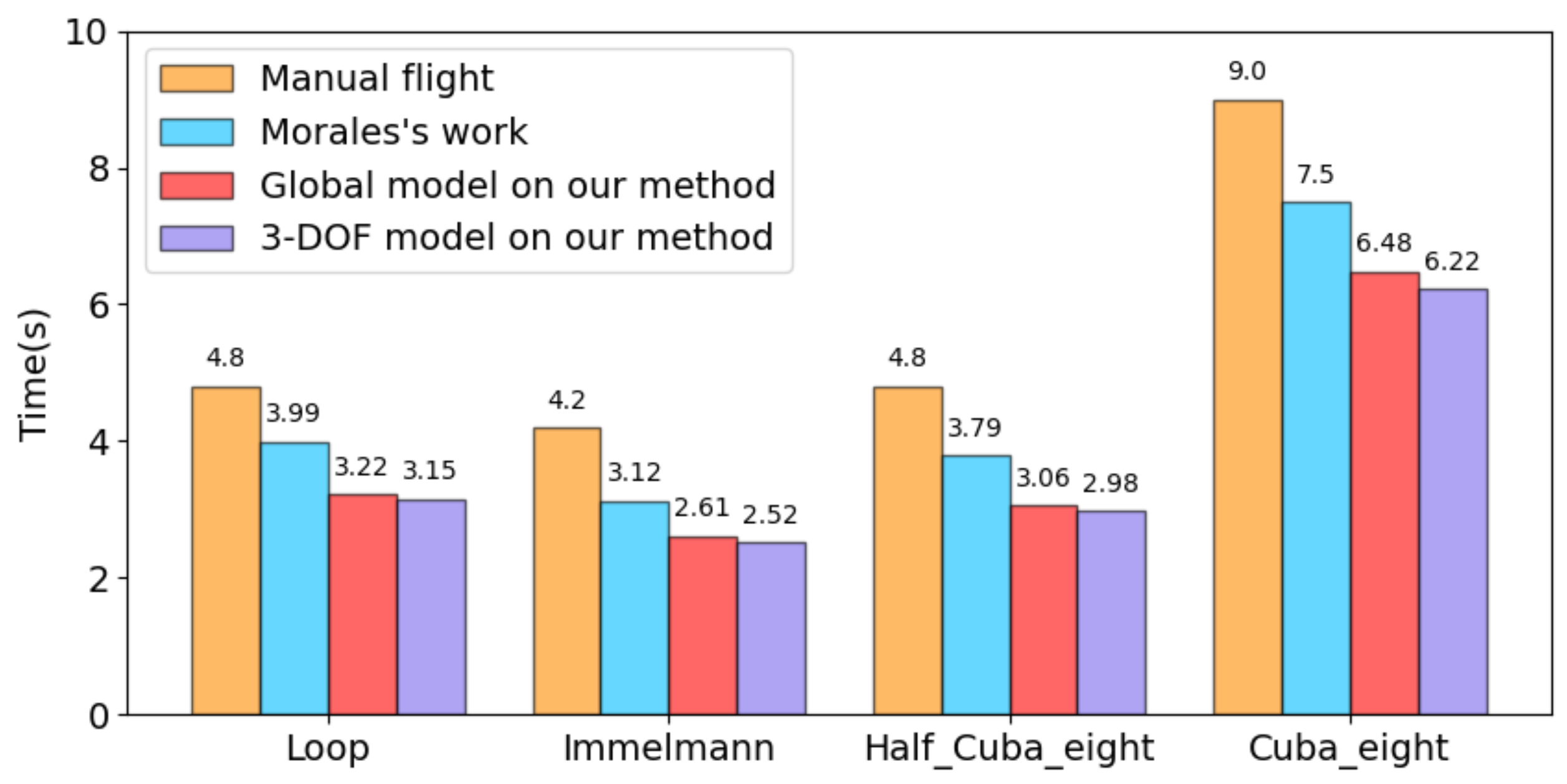
5.3. Benchmark Comparisons

To further illustrate the superiority of our approach, a comparison with three other methods is conducted. The first strategy is through collecting the maneuvering trajectories performed by the human pilot. The second one is the Gaussian pseudo-spectral method proposed in Morales’s work [24]. Moreover, the 3-DOF model introduced [23] was also utilized in our approach, formulated in Appendix B. The simulation results are depicted in the Figure 10.

On this basis, we list the statistical flight time data in the Figure 11 for quantitative comparison of each method.

It can be seen from Figure 10; Figure 11 that the trajectories obtained from manual flights are inferior to the other methods. Even though Morales’s method’s performance is slightly better than the manual flight, it cannot solve the period constraints. The flight time is significantly longer than those of our proposed method and the 3-DOF model. The method proposed in this paper was based on the global model, and motion segmentation is needed increasing computational costs. It is worth noting that our approach can flexibly connect those segments, resulting in various maneuvers. In the result of the mass point model, since our model was simplified, and there was no need to segment the trajectories, the maneuvering time optimized was slightly shorter than our method. Therefore, the optimization results based on the 3-DOF model can be utilized as an initial guess in our approach or for benchmark comparison. Since the 3-DOF model was simplified by ignoring the kinodynamic constraints, it cannot be directly used for maneuvering planning.

In order to conduct a more thorough analysis, we performed statistics on the running time of several methods. All the experiments were executed on an Intel Core i7-4710MQ CPU with 8 GB RAM that runs at 2.50 GHz.

It can be seen from

Table 5. Calculation efficiency comparison.

Acrobatic Maneuver and Methods	Morales’s Work	Proposed-Global Model	Proposed-3-DOF Model
Loop	20 min	10 min	45 s
Immelmann	6 min	2 min	48 s
Half Cuban eight	8 min	3 min	42 s
Cuban eight	20 min	8 min	2 min

that the minimal-time maneuver optimization is time-consuming. Our work decomposes the optimization into the calculation of the 3-DOF model (initial guess) and the re-optimization of the global model. Compared with Morales’s work, the optimized solution can be obtained faster.

5.4. Analysis of Maneuver Optimization Algorithm

It worth noting that the optimization process of maneuvers is quite time-consuming due to the inherent highly non-convex property. There are several methods that can accelerate the calculations and avoid the infeasible problem in Ipopt solver.

(1)

Global Fixed-wing model

Our optimization algorithm requires an accurate model in order to obtain the extreme motion of the UAV. Although the simplification of the model was conducive to simplifying the calculation, it was difficult to get the most realistic movement conditions. In our multiple maneuvering experiments, the performance of the drone was pushed to the limit, which was in line with the minimum time movement characteristics.

(2)

Key-frames and primitives design

To the best knowledge of the authors, it’s unfeasible to propose a unified approach of key-frame extraction and motion decomposition for various maneuvers. Choosing the number of the key-frames and primitives requires a balance between computational complexity and geometric accuracy. Furthermore, most of the maneuvers can be decomposed into several longitudinal and lateral primitives.

(3)

Initial guess

The initial guess is essential for the nonlinear programming problem. In this paper, a reasonable initial guess was obtained either from the optimization results based on the point-mass model (${\dot{p}}^i=a$, with input $u=a,‖a‖\le a_{\max }$) or simply from the demonstration data using interpolation.

(4)

Optimization constraints

The small slacking variables can be added into the nonlinear constraints to accelerate the calculation and avoid the infeasible solutions. For instance, the complimentary constraint can be adjusted into:

$$0\le {\mu }_k^i\cdot \left({‖p_k-p_i‖}_2-d{p}_k^i\right)\le {10}^{-3}$$

In addition, excessive slacking variables can be added into nonlinear constraints to obtain an initial solution, which can be considered as the initial guess in the next step of optimization iteratively.

6. Conclusions

In this paper, a hybrid-driven flight maneuver optimization framework was proposed. Based on the demonstrated maneuvers performed by an experienced pilot, the parameters of the UAV model along with the features of maneuvers were extracted. Then, the idea of key-frames and maneuver primitives were proposed which can design and concatenate different maneuvers more flexibly. Based on the above work, we formulated maneuver planning into a time-optimal problem, the feasibility of the framework was fully verified through designing the positional, attitude, and compound key-frames in the loop, Immelmann, half Cuban eight, and Cuban eight maneuvers. Through comparison, it can be concluded that the designed action was faster than professional pilots, and the results provide verifications on the optimality of the solutions and the effectiveness of the proposed approach.

Future works will concentrate on realizing our algorithm on a UAV platform experimentally.

References

1. Ju, C.; Son, H.I. Multiple UAV systems for agricultural applications: Control, implementation, and evaluation. Electronics 2018, 7, 162. [Google Scholar] [CrossRef] [Green Version]
2. Tang, T.; Hong, T.; Hong, H.; Ji, S.; Mumtaz, S.; Cheriet, M. An improved UAV-PHD filter-based trajectory tracking algorithm for multi-UAVs in future 5G IoT scenarios. Electronics 2019, 8, 1188. [Google Scholar] [CrossRef] [Green Version]
3. Zhou, Y.; Wu, C.; Wu, Q.; Eli, Z.M.; Xiong, N.; Zhang, S. Design and analysis of refined inspection of field conditions of oilfield pumping wells based on rotorcraft uav technology. Electronics 2019, 8, 1504. [Google Scholar] [CrossRef] [Green Version]
4. Chen, C.L.; Deng, Y.Y.; Weng, W.; Chen, C.H.; Chiu, Y.J.; Wu, C.M. A traceable and privacy-preserving authentication for UAV communication control system. Electronics 2020, 9, 62. [Google Scholar] [CrossRef] [Green Version]
5. Stellin, M.; Sabino, S.; Grilo, A. LoRaWAN Networking in Mobile Scenarios Using a WiFi Mesh of UAV Gateways. Electronics 2020, 9, 630. [Google Scholar] [CrossRef] [Green Version]
6. Mellinger, D.; Michael, N.; Kumar, V. Trajectory generation and control for precise aggressive maneuvers with quadrotors. Int. J. Robot. Res. 2012, 1–11. [Google Scholar] [CrossRef]
7. Hehn, M.; Ritz, R.; DAndrea, R. Performance benchmarking of quadrotor systems using time-optimal control. Auton. Robot. 2012, 33, 69–88. [Google Scholar] [CrossRef]
8. Kaufmann, E.; Loquercio, A.; Ranftl, R.; Muller, M.; Koltun, V.; Scaramuzza, D. Deep drone acrobatics. RSS: Robotics, Science, and Systems. arXiv 2021, arXiv:2006.05768. [Google Scholar]
9. Gilhyun, R.; Tal, E.; Karaman, S. Multi-fidelity black-box optimization for time-optimal quadrotor maneuvers. RSS: Robotics, Science, and Systems. arXiv 2020, arXiv:2006.02513. [Google Scholar]
10. Bry, A.; Richter, C.; Bachrach, A.; Roy, N. Aggressive flight of fixed-wing and quadrotor aircraft in dense indoor environments. Int. J. Robot. Res. 2015, 34, 969–1002. [Google Scholar] [CrossRef]
11. Levin, M. Maneuver Design and Motion Planning for Agile Fixed-Wing UAVs. Ph.D. Thesis, McGill University, Montreal, Canada, April 2019. [Google Scholar]
12. Tang, J.; Singh, A.; Goehausen, N. Parameterized Maneuver Learning for Autonomous Helicopter Flight. In Proceedings of the IEEE International Conference on Robotics and Automation, Anchorage, AK, USA, 4–8 May 2010. [Google Scholar]
13. Abbeel, P. Apprenticeship Learning and Reinforcement Learning with Application to Robotic Control. Ph.D. Thesis, Stanford University, Stanford, CA, USA, August 2008. [Google Scholar]
14. Abbeel, P.; Coates, A.; Ng, A.Y. Autonomous Helicopter Aerobatics through Apprenticeship Learning. Int. J. Robot. Res 2010, 29, 1608–1639. [Google Scholar] [CrossRef]
15. Mueller, M.W.; Hehn, M.; D′Andrea, R. A computationally efficient motion primitive for quadrocopter trajectory generation. IEEE Trans. Robot. 2015, 31, 1294–1310. [Google Scholar] [CrossRef]
16. Quan, L.; Han, L.; Zhou, B. Survey of UAV motion planning. IET Cyber-Syst. Robot. 2020, 2, 14–21. [Google Scholar] [CrossRef]
17. Liu, S.; Mohta, K.; Atanasov, N.; Kumar, V. Search-based motion planning for aggressive flight in se (3). IEEE Robot. Autom. Lett. 2018, 3, 2439–2446. [Google Scholar] [CrossRef] [Green Version]
18. Watterson, M.; Liu, S.; Sun, K.; Smith, T.; Kumar, V. Trajectory optimization on manifolds with applications to quadrotor systems. Int. J. Robot. Res. 2020, 39, 303–320. [Google Scholar] [CrossRef]
19. Wang, Z.; Zhou, X.; Xu, C.; Gao, F. Geometrically Constrained Trajectory Optimization for Multicopters. arXiv 2021, arXiv:2103.00190. [Google Scholar]
20. Basescu, M.; Moore, J. Direct nmpc for Post-Stall Motion Planning with Fixed-Wing uavs. In Proceedings of the 2020 IEEE International Conference on Robotics and Automation (ICRA), Paris, France, 31 May–31 August 2020. [Google Scholar]
21. Fan, Y.; Lutze, F.H.; Cliff, E.M. Time-optimal lateral maneuvers of an aircraft. J. Guid. Control. Dyn. 1995, 18, 1106–1112. [Google Scholar] [CrossRef]
22. Komduur, H.J.; Visser, H.G. Optimization of vertical plane cobralike pitch reversal maneuvers. J. Guid. Control. Dyn. 2002, 25, 693–702. [Google Scholar] [CrossRef]
23. Imado, F.; Heike, Y.; Kinoshita, T. Research on a new aircraft point-mass model. J. Aircr. 2011, 48, 1121–1130. [Google Scholar] [CrossRef]
24. Morales, M.A.; Silvestre, F.J.; Neto, A.B.G. Equations of motion for optimal maneuvering with global aerodynamic model. Aerosp. Sci. Technol. 2018, 77, 206–216. [Google Scholar] [CrossRef]
25. Du, D.; Qi, Y.; Yu, H. The Unmanned Aerial Vehicle Benchmark: Object Detection and Tracking. In Proceedings of the European Conference on Computer Vision (ECCV), Munich, Germany, 8–14 September 2018. [Google Scholar]
26. Wen, L.; Zhu, P.; Du, D. Visdrone-sot2018: The Vision Meets Drone Single-Object Tracking Challenge Results. In Proceedings of the European Conference on Computer Vision (ECCV), Munich, Germany, 8–14 September 2018. [Google Scholar]
27. Qi, Y.; Wu, Q.; Anderson, P. Reverie: Remote Embodied Visual Referring Expression in Real Indoor Environments. In Proceedings of the IEEE/CVF Conference on Computer Vision and Pattern Recognition, Seattle, WA, USA, 14–19 June 2020. [Google Scholar]
28. Hong, Y.; Rodriguez-Opazo, C.; Qi, Y. Language and visual entity relationship graph for agent navigation. arXiv 2020, arXiv:2010.09304. [Google Scholar]
29. Qi, Y.; Pan, Z.; Hong, Y.; Yang, M.H.; Hengel, A.; Wu, Q. Know What and Know Where: An Object-and-Room Informed Sequential BERT for Indoor Vision-Language Navigation. arXiv 2021, arXiv:2104.04167. [Google Scholar]
30. Qi, Y.; Pan, Z.; Zhang, S. Object-and-action aware model for visual language navigation. In Proceedings of the Computer Vision–ECCV 2020: 16th European Conference, Glasgow, UK, 23–28 August 2020. [Google Scholar]
31. Gebhardt, C.; Hepp, B.; Nägeli, T. Airways: Optimization-based Planning of Quadrotor Trajectories According to High-Level User Goals. In Proceedings of the 2016 CHI Conference on Human Factors in Computing Systems, San Jose, CA, USA, 7–12 May 2016. [Google Scholar]
32. Mellinger, D.; Kumar, V. Minimum Snap Trajectory Generation and Control for Quadrotors. In Proceedings of the 2011 IEEE International Conference on Robotics and Automation, Shanghai, China, 9–13 May 2011. [Google Scholar]
33. Foehn, P.; Davide, S. CPC: Complementary progress constraints for time-optimal quadrotor trajectories. arXiv 2020, arXiv:2007.06255. [Google Scholar]
34. Foehn, P.; Romero, A.; Scaramuzza, D. Time-optimal planning for quadrotor waypoint flight. Sci. Robot. 2021, 6, eabh1221. [Google Scholar] [CrossRef]
35. Rousseau, G.; Maniu, C.S.; Tebbani, S.; Babel, M.; Martin, N. Minimum-time B-spline trajectories with corridor constraints. Application to cinematographic quadrotor flight plans. Control. Eng. Pract. 2019, 89, 190–203. [Google Scholar] [CrossRef] [Green Version]
36. Frazzoli, E.; Dahleh, M.A.; Feron, E. Maneuver-Based Motion Planning for Nonlinear Systems with Symmetries. IEEE Trans. Robot. 2005, 21, 1077–1091. [Google Scholar] [CrossRef]
37. Bulka, E.; Nahon, M. Autonomous Fixed-Wing Aerobatics: From Theory to Flight. In Proceedings of the 2018 IEEE International Conference on Robotics and Automation (ICRA), Brisbane, Australia, 21–25 May 2018. [Google Scholar]
38. Bulka, E.; Nahon, M. Automatic Control for Aerobatic Maneuvering of Agile Fixed-Wing UAVs. J. Intell. Robot. Syst. 2019, 93, 85–100. [Google Scholar] [CrossRef]
39. Levin, J.M.; Nahon, M.; Paranjape, A.A. Real-time motion planning with a fixed-wing UAV using an agile maneuver space. Auton. Robot. 2019, 43, 2111–2130. [Google Scholar] [CrossRef]
40. Wang, B.; Gong, J.; Chen, H. Motion Primitives Representation, Extraction and Connection for Automated Vehicle Motion Planning Applications. IEEE Trans. Intell. Transp. Syst. 2020, 21, 3931–3945. [Google Scholar] [CrossRef]
41. Zhang, R.; Hu, Y.; Zhao, K. A Novel Dual Quaternion Based Dynamic Motion Primitives for Acrobatic Flight. In Proceedings of the 2021 5nd International Conference on Robotics and Automation Sciences (ICRAS), Wuhan, China, 11–13 June 2021. [Google Scholar]
42. Sonneveldt, L. “Nonlinear F-16 Model Description”,Control and Simulation Div. Faculty of Aerospace Engineering; Delft University of Technology: Delft, The Netherlands, 2006. [Google Scholar]
43. Zhang, R.; Zhang, J.; Yu, H. Review of Modeling and Control in UAV Autonomous Maneuvering Flight. In Proceedings of the 2018 IEEE International Conference on Mechatronics and Automation (ICMA), Changchun, China, 5–8 August 2018. [Google Scholar]
44. Dutra, D.A. Collocation-Based Output-Error Method for Aircraft System Identification. In Proceedings of the AIAA Aviation 2019 Forum, Dallas, TX, USA, 17–21 June 2019. [Google Scholar]
45. Andersson, J.; Joris, G.; Horn, G.; Rawlings, J.B.; Diehl, M. CasADi: A software framework for nonlinear optimization and optimal control. Math. Program. Comput. 2018, 11, 1–36. [Google Scholar] [CrossRef]
46. Wächter, A.; Biegler, L.T. On the implementation of an interior-point filter line-search algorithm for large-scale nonlinear programming. Math. Program. 2006, 106, 25–57. [Google Scholar] [CrossRef]
Figure 1. Hybrid-driven optimal maneuvering flight planning framework. We start with pilot demonstration and maneuver data collection and then perform model identification and maneuver key-frame and motion primitive analysis. Finally, based on the global model and key-frames, the optimal primitives are generated, and the corresponding primitives are concatenated into a complete maneuver.
Electronics 10 02330 g001
Figure 2. A typical maneuvering flight. The UAV has experienced multiple different position and attitude changes in a continuous period of time.
Electronics 10 02330 g002
Figure 3. Flight maneuver demonstration and learning system including (1) remote controller, (2) signal receiver, (3) Pixhawk-v5, (4) flight joystick, (5) ground control station, and (6) flight simulation software X-Plane.
Electronics 10 02330 g003
Figure 4. Some typical maneuver teaching data. The pilot performed different maneuvers continuously over a period of time, which is marked with different colors.
Electronics 10 02330 g004
Figure 5. These figures show the key-frame-based optimization problem. The drone is required to sequentially pass through several different types of key-frames within a period of time, marked with different colors. We show the changes in the process state variables and process change variables in the process.
Electronics 10 02330 g005
Figure 6. The experiment results for the loop maneuver including state variables, control inputs, process state variables, and maneuvering trajectory. The thrust shrunk by a factor of 100, and the state at the positional key-frame is marked with a circle. In some cases, the roll angle and yaw angle jumped between 180 and −180. (h) is the trajectory of UAV loop maneuver, including UAVs with different attitudes, the characteristic points are marked with different shapes.
Electronics 10 02330 g006aElectronics 10 02330 g006b
Figure 7. The experimental results for the Immelmann maneuver including state variables, control inputs, process state variables, and maneuvering trajectory. The thrust shrunk by a factor of 100, and the half loop primitive is represented by a solid line, the roll primitive is represented by a dashed line, the state at the attitude key-frame is marked by a diamond, and the red, dashed line represented the connection of the primitive. It should be noted that different primitives have different process change variables. (h) is the trajectory of UAV Immelmann maneuver, including UAVs with different attitudes, the characteristic points are marked with different shapes.
Electronics 10 02330 g007aElectronics 10 02330 g007b
Figure 8. The experiment results for the half Cuban eight maneuver including state variables, control inputs, process state variables, and maneuvering trajectory. The thrust shrunk by a factor of 100, and the half loop primitive is represented by a solid line, the special rolling primitive is represented by a dashed line, the compound key-frame is marked with a pentacle. (h) is the trajectory of UAV half Cuban eight maneuver, including UAVs with different attitudes, the characteristic points are marked with different shapes.
Electronics 10 02330 g008aElectronics 10 02330 g008b
Figure 9. The experiment results for the Cuban eight maneuver including state variables, control inputs, process state variables, and maneuvering trajectory. The whole maneuver contains four primitives, the two loop parts are represented by solid lines, and the rolling part is represented by dashed lines. (h) is the trajectory of UAV Cuban eight maneuver, including UAVs with different attitudes, the characteristic points are marked with different shapes.
Electronics 10 02330 g009aElectronics 10 02330 g009b
Figure 10. Comparison of maneuvering trajectories optimized by four methods. The magenta, red, sky blue, and blue curves represent manual flight, proposed approach, 3-DOF model, and Morales’s method, respectively.
Electronics 10 02330 g010aElectronics 10 02330 g010b
Figure 11. The time characteristics of different methods in different maneuvers, the orange, red, purple, and blue box represent manual flight, proposed approach, 3-DOF model, and Morales’s method, respectively.
Electronics 10 02330 g011