
Acoustic Anomaly Detection of Mechanical Failures in Noisy Real-Life Factory Environments


Abstract
:1. Introduction
2. Related Works
2.1. Analysis of Industrial Machinery Data for Predictive Maintenance
2.2. Signal Processing Based Methods
2.3. Machine Learning-Based Methods
2.4. Deep Learning-Based Methods
2.5. Generative Adversarial Network-Based Methods
3. Materials and Methods
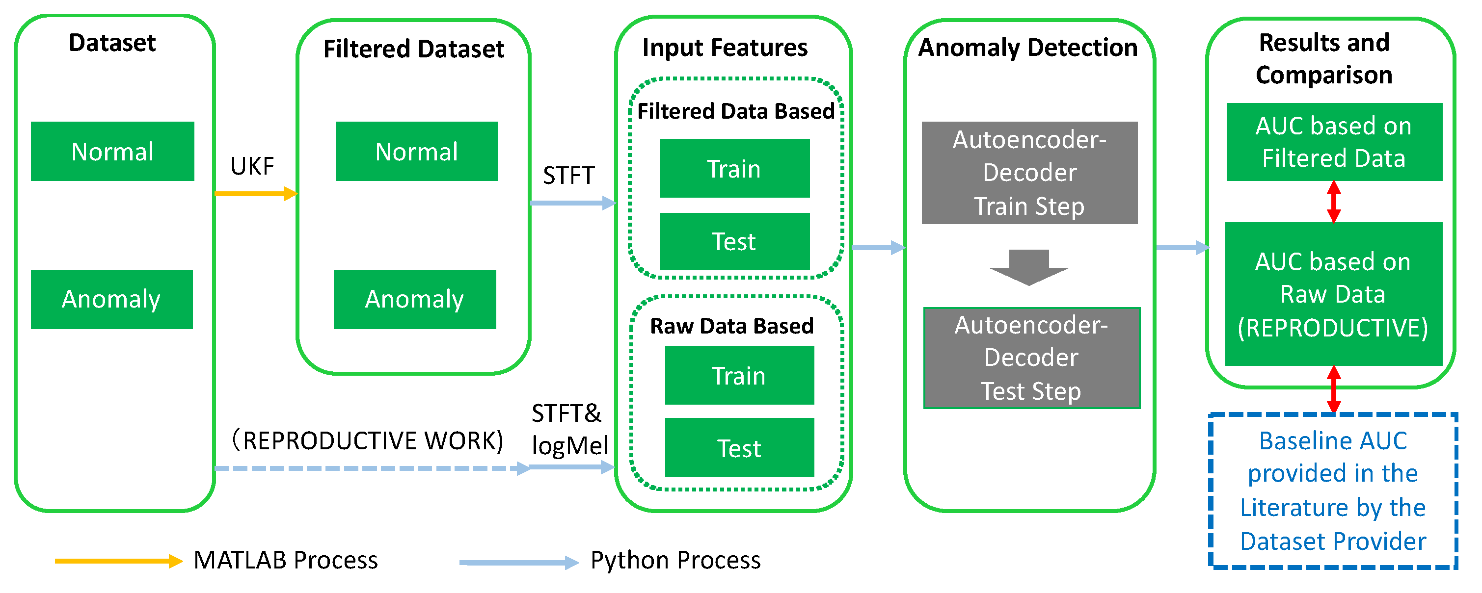
3.1. Methodology
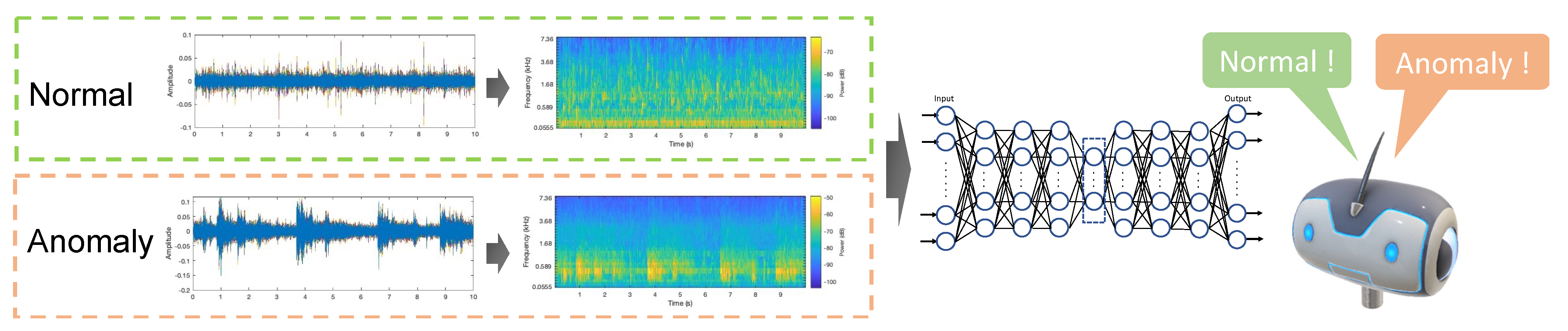
3.2. Datasets
3.3. Feature Engineering
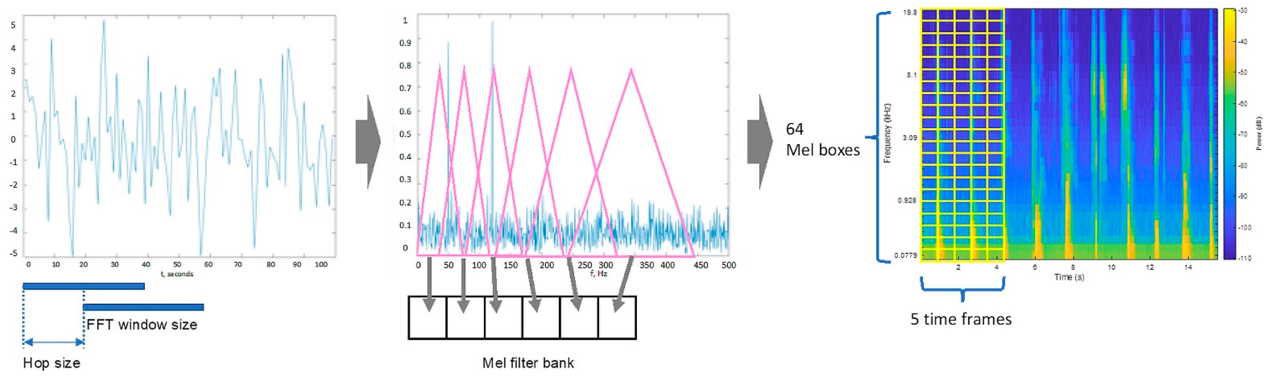
3.4. Problem Formulation and Signal Processing
3.5. Signal Processing
3.6. Dimension Reduction with PCA and T-SNE
3.7. One-Class Support Vector Machine (OC-SVM)
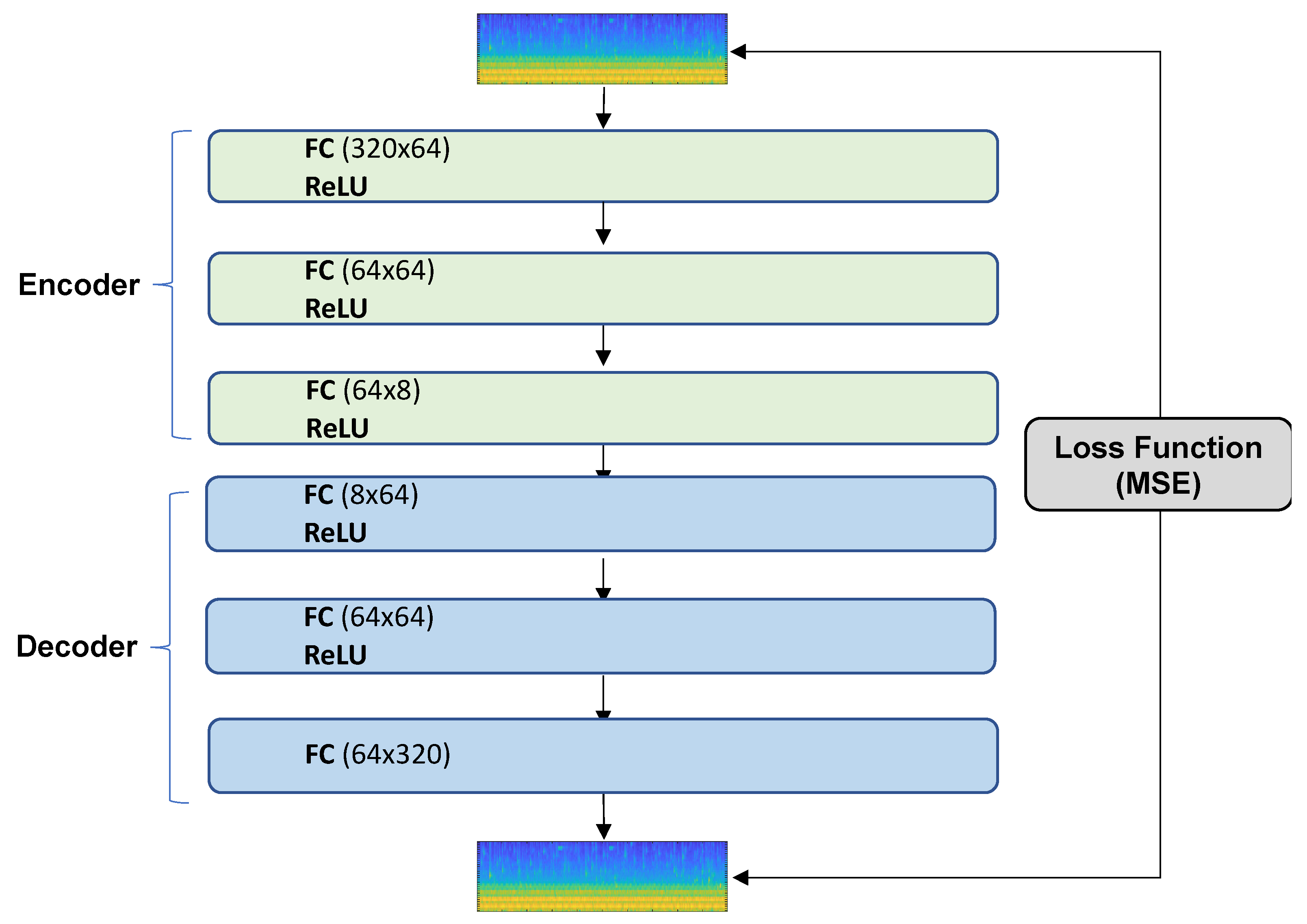
3.8. Autoencoder-Decoder Neural Network
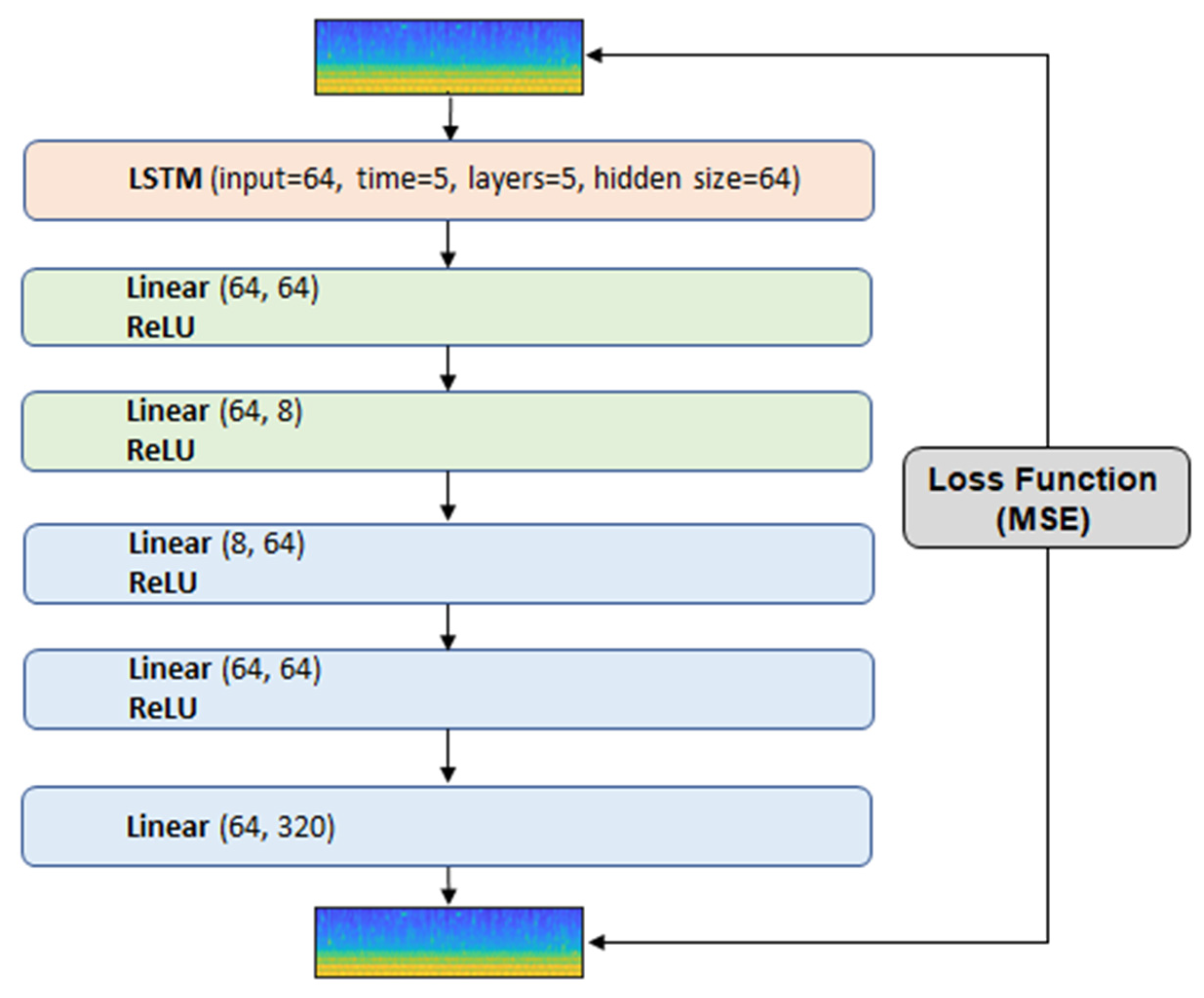
3.9. Neural Network Auto-Encoder-Decoder with LSTM
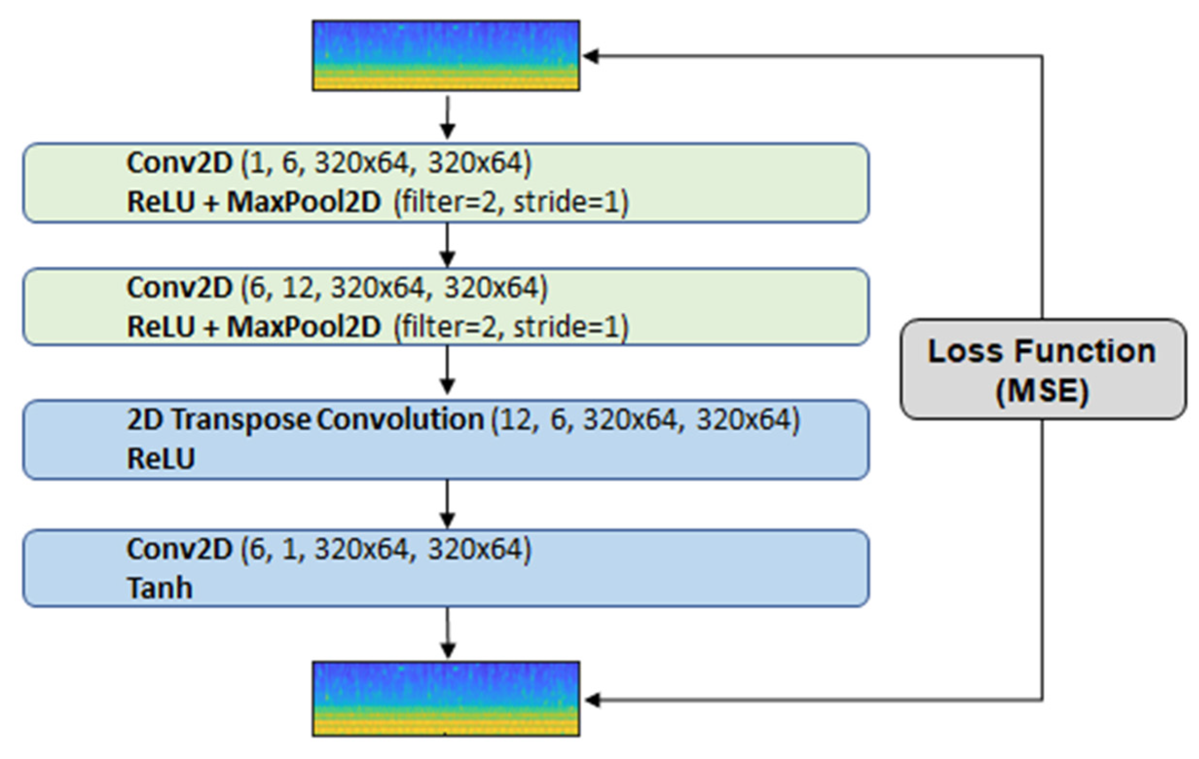
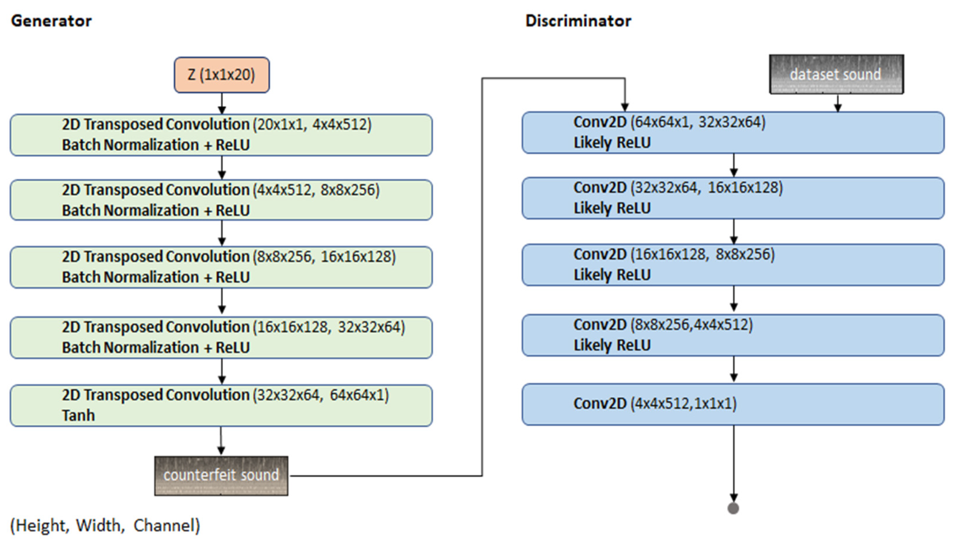
3.10. Generative Adversarial Network
3.11. Optimization
3.12. Evaluation
3.13. Development Environment
4. Experimental Analysis
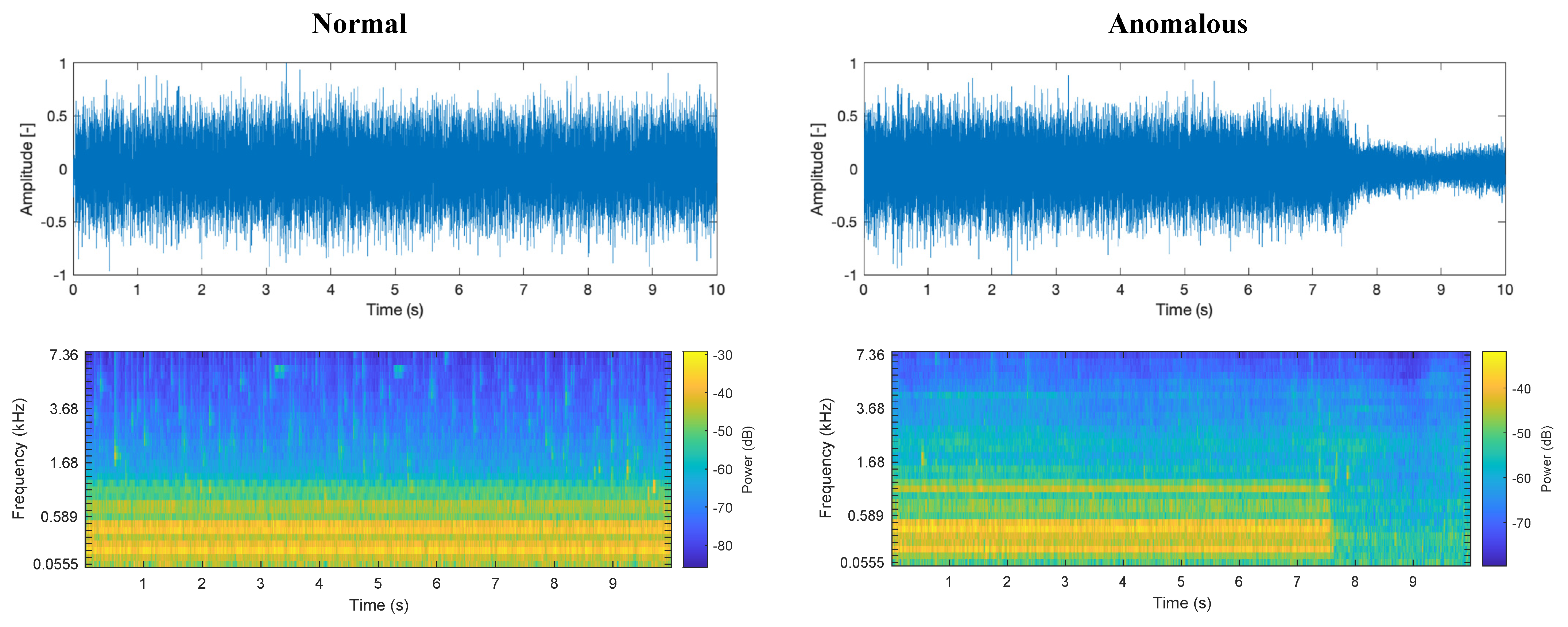
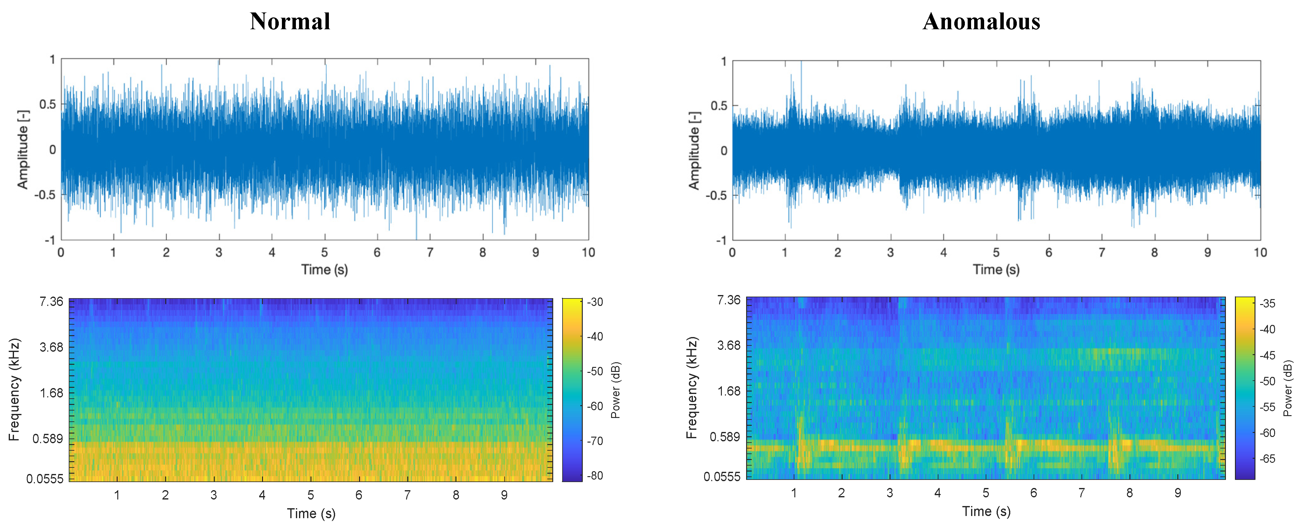
4.1. Data Analysis
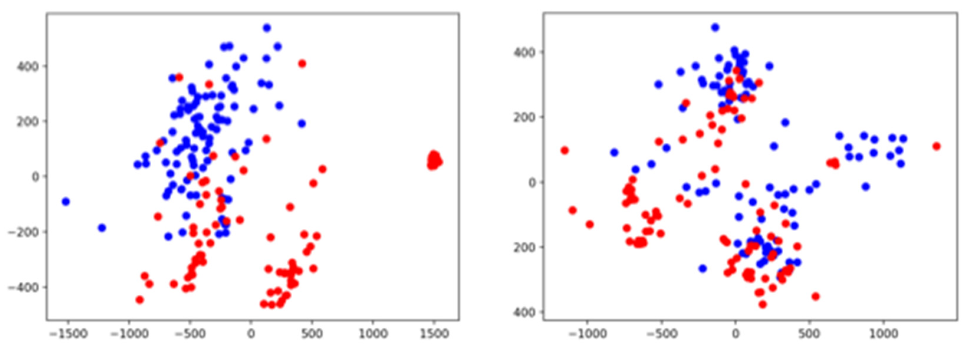
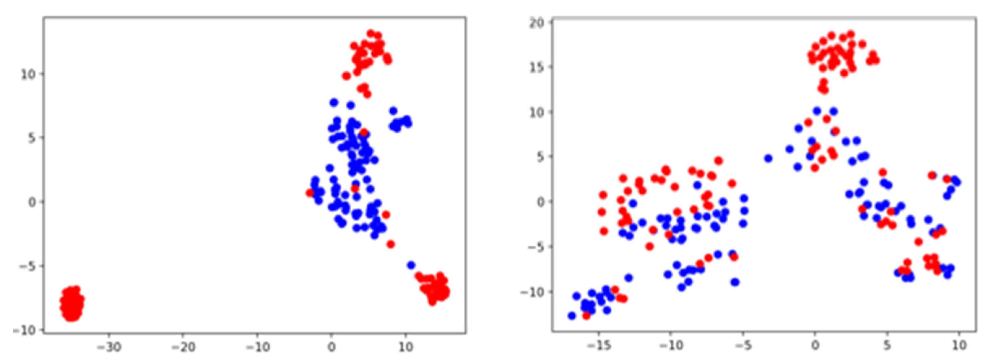
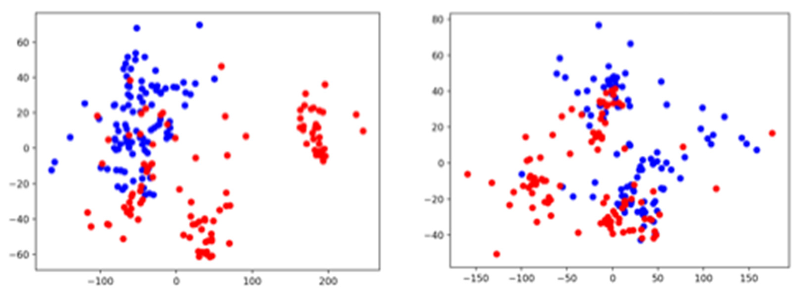
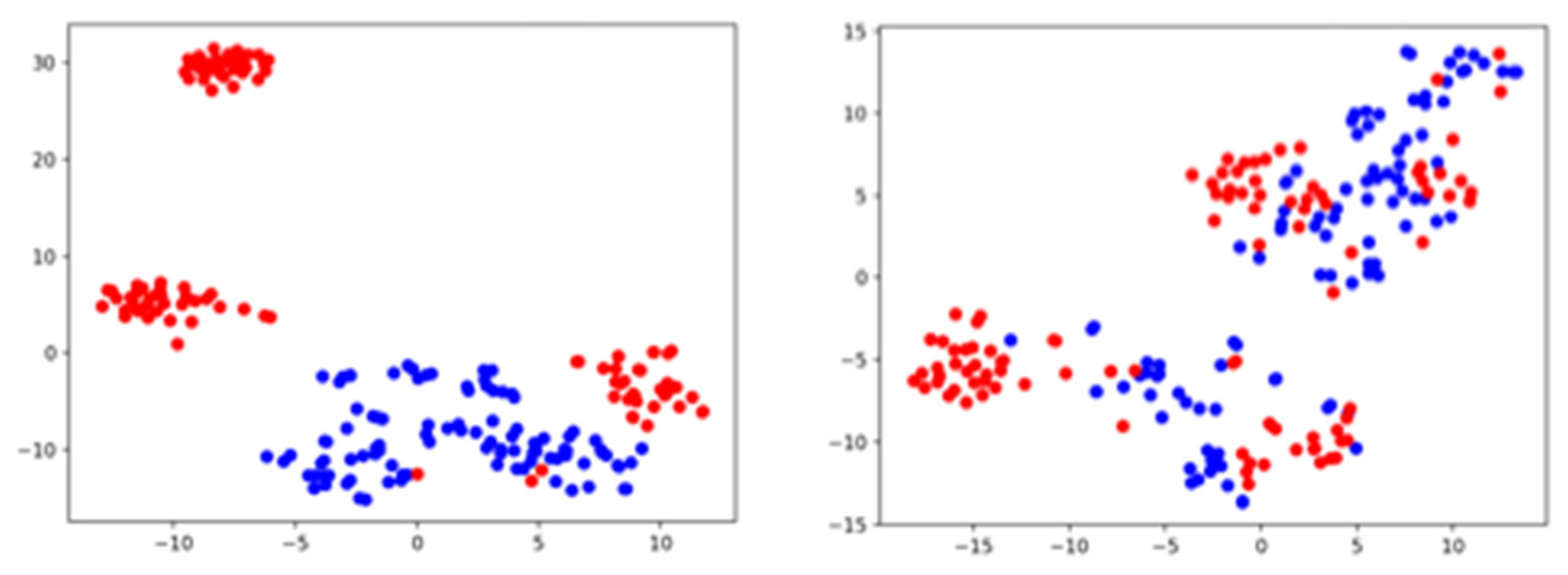
4.2. Results of Dimensionality Reduction
4.3. Results of the Autoencoder as the Baseline Model
4.4. Results of the One-Class Support Vector Machine as a Baseline Model
4.5. Results of the Autoencoder with LSTM
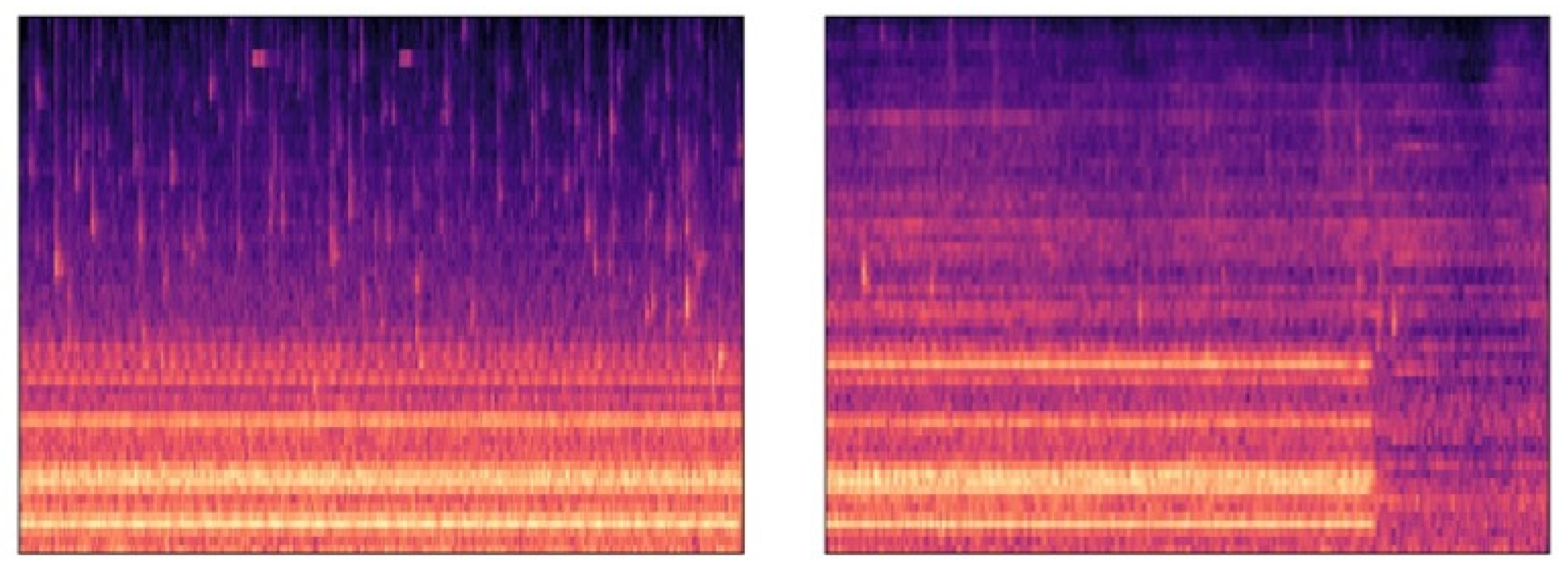
4.6. Results of the Generative Adversarial Network for Anomaly Detection (ANOGAN)
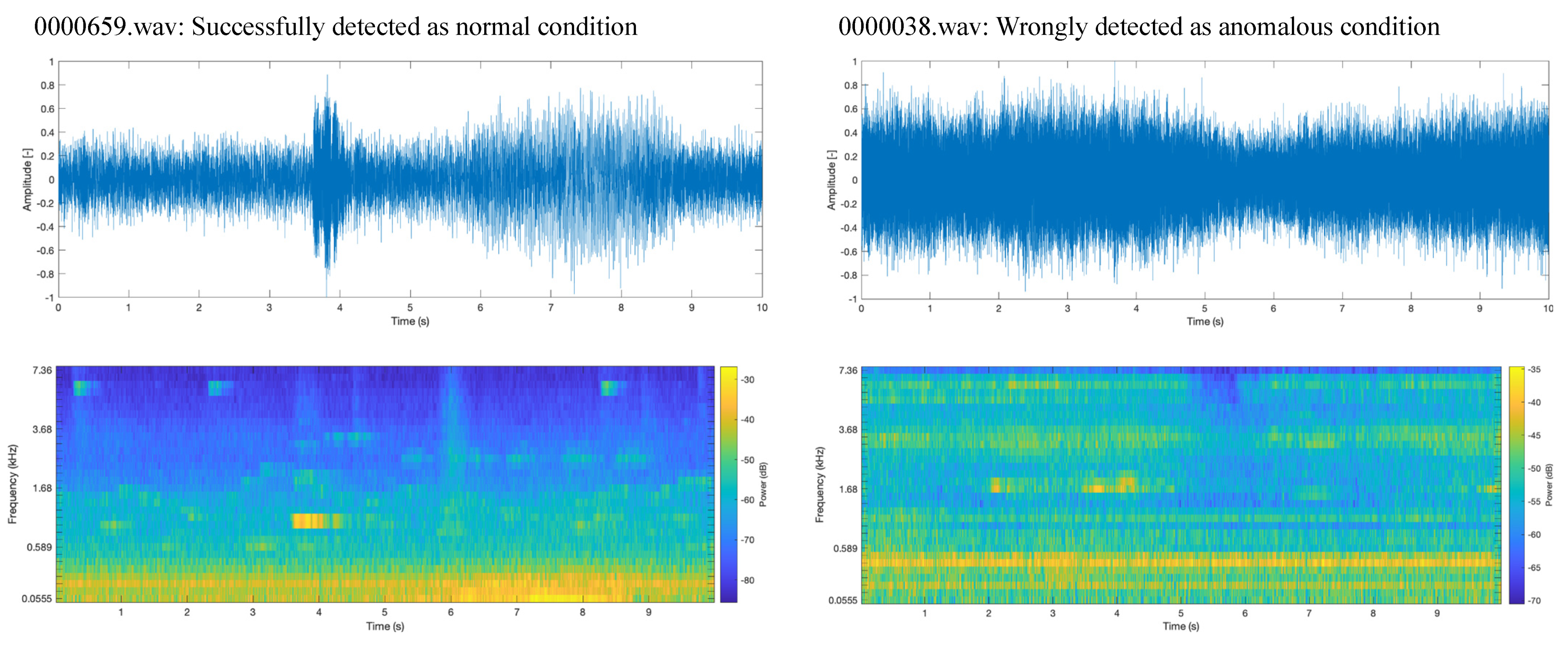
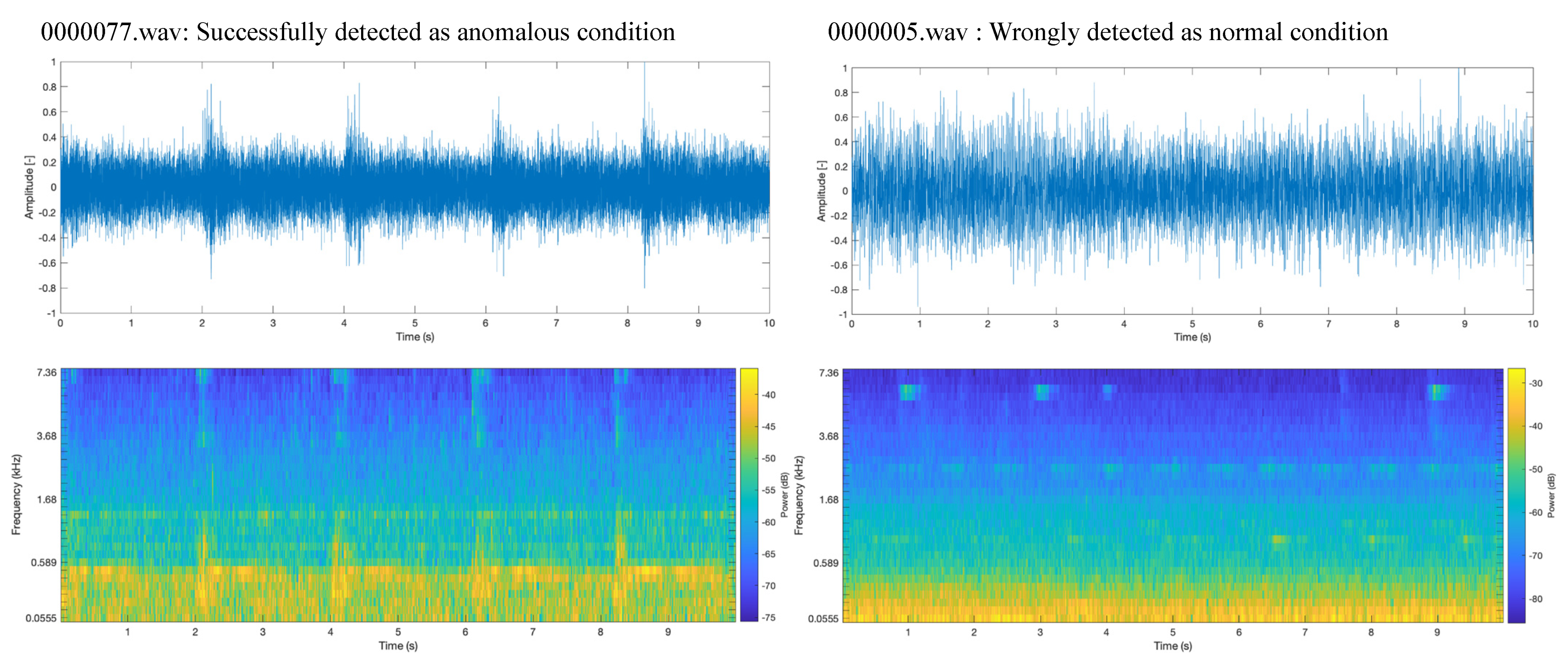
4.7. Analysis of Misclassifications
5. Discussion and Comparison with Similar Works
6. Conclusions and Future Work
Author Contributions
Funding
Data Availability Statement
Acknowledgments
Conflicts of Interest
References
- Chandola, V.; Banerjee, A.; Kumar, V. Anomaly detection: A survey. ACM Comput. Surv. 2009, 41, 1–58. [Google Scholar] [CrossRef]
- Çınar, Z.M.; Nuhu, A.A.; Zeeshan, Q.; Korhan, O.; Asmael, M.; Safaei, B. Machine learning in predictive maintenance towards sustainable smart manufacturing in industry 4.0. Sustainability 2020, 12, 8211. [Google Scholar] [CrossRef]
- An, Q.; Tao, Z.; Xu, X.; El Mansori, M.; Chen, M. A data-driven model for milling tool remaining useful life prediction with convolutional and stacked LSTM network. Measurement 2020, 15, 107461. [Google Scholar] [CrossRef]
- Lv, Y.; Liu, Y.; Jing, W.; Woźniak, M.; Damaševičius, R.; Scherer, R.; Wei, W. Quality control of the continuous hot pressing process of medium density fiberboard using fuzzy failure mode and effects analysis. Appl. Sci. 2020, 10, 4627. [Google Scholar] [CrossRef]
- Kawaguchi, Y.; Endo, T. How can we detect anomalies from subsampled audio signals? In Proceedings of the 2017 IEEE International Workshop on Machine Learning for Signal Processing, Tokyo, Japan, 25–28 September 2017. [Google Scholar] [CrossRef]
- Kawaguchi, Y. Anomaly detection based on feature reconstruction from subsampled audio signals. In Proceedings of the 26th European Signal Processing Conference (EUSIPCO), Rome, Italy, 3–8 September 2018; pp. 2538–2542. [Google Scholar]
- Marchie, E.; Vesperini, F.; Eyben, F.; Squartini, S.; Schuller, B. A novel approach for automatic acoustic novelty detection using a denoising autoencoder with bidirectional LSTM neural networks. In Proceedings of the International Conference on Acoustics, Speech, and Signal Processing (ICASSP), South Brisbane, Australia, 19–24 April 2015; pp. 1996–2000. [Google Scholar]
- Koizumi, Y.; Saito, S.; Uematsu, H.; Harada, N. Optimizing acoustic feature extractor for anomalous sound detection based on Neyman-Pearson lemma. In Proceedings of the 25th European Signal Processing Conference (EUSIPCO), Kos, Greece, 28 August–2 September 2017; pp. 698–702. [Google Scholar]
- Licitra, G.; Fredianelli, L.; Petri, D.; Vigotti, M.A. Annoyance evaluation due to overall railway noise and vibration in Pisa urban areas. Sci. Total Environ. 2016, 568, 1315–1325. [Google Scholar] [CrossRef]
- Miedema, H.M.E.; Oudshoorn, C.G.M. Annoyance from transportation noise: Relationships with exposure metrics DNL and DENL and their confidence intervals. Environ. Health Perspect. 2001, 109, 409–416. [Google Scholar] [CrossRef]
- Vukić, L.; Fredianelli, L.; Plazibat, V. Seafarers’ Perception and attitudes towards noise emission on board ships. Int. J. Environ. Res. Public Health 2021, 18, 6671. [Google Scholar] [CrossRef]
- Rossi, L.; Prato, A.; Lesina, L.; Schiavi, A. Effects of low-frequency noise on human cognitive performances in laboratory. Build. Acoust. 2018, 25, 17–33. [Google Scholar] [CrossRef]
- Minichilli, F.; Gorini, F.; Ascari, E.; Bianchi, F.; Coi, A.; Fredianelli, L.; Licitra, G.; Manzoli, F.; Mezzasalma, L.; Cori, L. Annoyance judgment and measurements of environmental noise: A focus on Italian secondary schools. Int. J. Environ. Res. Public Health 2018, 15, 208. [Google Scholar] [CrossRef] [Green Version]
- Erickson, L.C.; Newman, R.S. Influences of background noise on infants and children. Curr. Dir. Psychol. Sci. 2017, 26, 451–457. [Google Scholar] [CrossRef]
- Dratva, J.; Phuleria, H.C.; Foraster, M.; Gaspoz, J.M.; Keidel, D.; Künzli, N.; Liu, L.J.; Pons, M.; Zemp, E.; Gerbase, M.W.; et al. Transportation noise and blood pressure in a population-based sample of adults. Environ. Health Perspect. 2012, 120, 50–55. [Google Scholar] [CrossRef]
- Petri, D.; Licitra, G.; Vigotti, M.A.; Fredianelli, L. Effects of exposure to road, railway, airport and recreational noise on blood pressure and hypertension. Int. J. Environ. Res. Public Health 2021, 18, 9145. [Google Scholar] [CrossRef]
- Babisch, W.; Beule, B.; Schust, M.; Kersten, N.; Ising, H. Traffic noise and risk of myocardial infarction. Epidemiology 2005, 16, 33–40. [Google Scholar] [CrossRef]
- Ajitha, P.; Chandra, E. Survey on outliers detection in distributed data mining for big data. J. Basic Appl. Sci. Res. 2015, 5, 31–38. [Google Scholar]
- Calabrese, F.; Regattieri, A.; Bortolini, M.; Gamberi, M.; Pilati, F. Predictive maintenance: A novel framework for a data-driven, semi-supervised, and partially online prognostic health management application in industries. Appl. Sci. 2021, 11, 3380. [Google Scholar] [CrossRef]
- Tanuska, P.; Spendla, L.; Kebisek, M.; Duris, R.; Stremy, M. Smart anomaly detection and prediction for assembly process maintenance in compliance with industry 4.0. Sensors 2021, 21, 2376. [Google Scholar] [CrossRef]
- Peng, C.-Y.; Raihany, U.; Kuo, S.-W.; Chen, Y.-Z. Sound detection monitoring tool in CNC milling sounds by K-means clustering algorithm. Sensors 2021, 21, 4288. [Google Scholar] [CrossRef]
- Kim, D.; Lee, S.; Kim, D. An applicable predictive maintenance framework for the absence of run-to-failure data. Appl. Sci. 2021, 11, 5180. [Google Scholar] [CrossRef]
- Skoczylas, A.; Stefaniak, P.; Anufriiev, S.; Jachnik, B. Belt conveyors rollers diagnostics based on acoustic signal collected using autonomous legged inspection robot. Appl. Sci. 2021, 11, 2299. [Google Scholar] [CrossRef]
- Ho, S.K.; Nedunuri, H.C.; Balachandran, W.; Kanfoud, J.; Gan, T.-H. Monitoring of industrial machine using a novel blind feature extraction approach. Appl. Sci. 2021, 11, 5792. [Google Scholar] [CrossRef]
- Mey, O.; Schneider, A.; Enge-Rosenblatt, O.; Mayer, D.; Schmidt, C.; Klein, S.; Herrmann, H.-G. Condition monitoring of drive trains by data fusion of acoustic emission and vibration sensors. Processes 2021, 9, 1108. [Google Scholar] [CrossRef]
- Serradilla, O.; Zugasti, E.; Ramirez de Okariz, J.; Rodriguez, J.; Zurutuza, U. Adaptable and explainable predictive maintenance: Semi-supervised deep learning for anomaly detection and diagnosis in press machine data. Appl. Sci. 2021, 11, 7376. [Google Scholar] [CrossRef]
- Wei, Y.; Li, Y.; Xu, M.; Huang, W. A review of early fault diagnosis approaches and their applications in rotating machinery. Entropy 2019, 21, 409. [Google Scholar] [CrossRef] [PubMed] [Green Version]
- Saufi, S.R.; Ahmad, Z.A.B.; Leong, M.S.; Lim, M.H. Challenges and opportunities of deep Learning models for machinery fault detection and diagnosis: A Review. IEEE Access 2019, 7, 122644. [Google Scholar] [CrossRef]
- Wang, D.; Brown, G.J. Computational Auditory Scene Analysis: Principles, Algorithms, and Applications; Wiley/IEEE Press: Piscataway, NJ, USA, 2006. [Google Scholar]
- Williamson, D.S.; Wang, D. Speech dereverberation and denoising using complex ratio masks. In Proceedings of the 2017 IEEE International Conference on Acoustics, Speech and Signal Processing (ICASSP), New Orleans, LA, USA, 5–9 March 2017; pp. 5590–5594. [Google Scholar] [CrossRef]
- Ayhan, B.; Kwan, C. Robust speaker identification algorithms and results in noisy environments; Lecture Notes in Computer Science. In Proceedings of the Advances in Neural Networks—ISNN 2018, Minsk, Belarus, 25–28 June; Huang, T., Lv, J., Sun, C., Tuzikov, A., Eds.; Springer: Cham, Switzerland; Volume 10878, pp. 443–450.
- Zhang, M.; Guo, J.; Li, X.; Jin, R. Data-driven anomaly detection approach for time-series streaming data. Sensors 2020, 20, 5646. [Google Scholar] [CrossRef] [PubMed]
- Pittino, F.; Puggl, M.; Moldaschl, T.; Hirschl, C. Automatic anomaly detection on in-production manufacturing machines using statistical learning methods. Sensors 2020, 20, 2344. [Google Scholar] [CrossRef] [PubMed] [Green Version]
- Hyvarinen, A.; Karhunen, H.; Oja, E. Independent Component Analysis; Wiley-Interscience: Hoboken, NJ, USA, 2001. [Google Scholar]
- Ikeda, S.; Toyama, K. Independent component analysis for noisy data—MEG data analysis. Neural Netw. 2000, 13, 1063–1074. [Google Scholar] [CrossRef]
- Koganeyama, M. An effective evaluation function for ICA to separate train noise from telluric current data. In Proceedings of the 4th International Symposium on Independent Component Analysis and Blind Signal Separation (ICA2003), Nara, Japan, 1–4 April 2003; pp. 837–842. [Google Scholar]
- Damaševičius, R.; Napoli, C.; Sidekerskienė, T.; Woźniak, M. IMF mode demixing in EMD for jitter analysis. J. Comput. Sci. 2017, 22, 240–252. [Google Scholar] [CrossRef]
- Kebabsa, T.; Ouelaa, N.; Djebala, A. Experimental vibratory analysis of a fan motor in industrial environment. Int. J. Adv. Manuf. Technol. 2018, 98, 2439–2447. [Google Scholar] [CrossRef]
- Garnier, J.; Solna, K. Applications of random matrix theory for sensor array imaging with measurement noise. Random Matrices 2014, 65, 223–245. [Google Scholar]
- Gu, X.; Akoglu, L.; Rinaldo, A. Statistical analysis of nearest neighbor methods for anomaly detection. In Proceedings of the 33rd Conference on Neural Information Processing Systems (NeurIPS 2019), Vancouver, BC, Canada, 8–14 December 2019; pp. 10921–10931. [Google Scholar]
- Scholkopf, B.; Williamson, R.; Smola, A.; Shawe-Taylor, J.; Platt, J. Support vector method for novelty detection. In Proceedings of the 12th International Conference on Neural Information Processing Systems (NIPS′99), Denver, CO, USA, 29 November–4 December 1999; pp. 582–588. [Google Scholar]
- Hsu, J.; Wang, Y.; Lin, K.; Chen, M.; Hsu, J.H. Wind turbine fault diagnosis and predictive maintenance through statistical process control and machine learning. IEEE Access 2020, 8, 23427–23439. [Google Scholar] [CrossRef]
- Toma, R.N.; Prosvirin, A.E.; Kim, J. Bearing fault diagnosis of induction motors using a genetic algorithm and machine learning classifiers. Sensors 2020, 20, 1884. [Google Scholar] [CrossRef] [Green Version]
- Sakurada, M.; Yairi, T. Anomaly detection using autoencoders with nonlinear dimensionality reduction. In Proceedings of the MLSDA 2014 2nd Workshop on Machine Learning for Sensory Data Analysis, Gold Coast, Australia, 2 December 2014; pp. 4–11. [Google Scholar]
- Ruff, L.; Vandermeulen, R.; Goernitz, N.; Deecke, L.; Siddiqui, S.A.; Binder, A.; Müller, E.; Kloft, M. Deep one-class classification. In Proceedings of the 35th International Conference on Machine Learning, Stockholm, Sweden, 10–15 July 2018; pp. 4393–4402. [Google Scholar]
- Luwei, K.C.; Yunusa-Kaltungo, A.; Sha’aban, Y.A. Integrated fault detection framework for classifying rotating machine faults using frequency domain data fusion and artificial neural networks. Machines 2018, 6, 59. [Google Scholar] [CrossRef] [Green Version]
- Zhao, H.; Liu, H.; Hu, W.; Yan, X. Anomaly detection and fault analysis of wind turbine components based on deep learning network. Renew. Energy 2018, 127, 825–834. [Google Scholar] [CrossRef]
- Dongo, Y.; Il, D.Y. Residual error based anomaly detection using auto-encoder in SMD machine sound. Sensors 2018, 18, 5. [Google Scholar]
- Cheng, Y.; Zhu, H.; Wu, J.; Shao, X. Machine health monitoring using adaptive kernel spectral clustering and deep long short-term memory recurrent neural networks. IEEE Trans. Ind. Inform. 2019, 15, 987–997. [Google Scholar] [CrossRef]
- Li, M.; Wang, S.; Fang, S.; Zhao, J. Anomaly detection of wind turbines based on deep small-world neural network. Appl. Sci. 2020, 10, 1243. [Google Scholar] [CrossRef] [Green Version]
- Chalapathy, R.; Chawla, S. Deep learning for anomaly detection: A Survey. arXiv 2019, arXiv:1901.03407v2. [Google Scholar]
- Goodfellow, I.J.; Pouget-Abadie, J.; Mirza, M.; Xu, B.; Warde-Farley, D.; Ozair, S.; Courville, A.; Bengio, Y. Generative adversarial nets. Adv. Neural Inform. Process. Syst. 2014, 27, 1–9. [Google Scholar]
- Schlegl, T.; Seeböck, P.; Waldstein, S.M.; Schmidt-Erfurth, U.; Langs, G. Unsupervised anomaly detection with generative adversarial networks to guide maker discovery. In Proceedings of the Information Processing in Medical Imaging 2017, Boone, NC, USA, 25–30 June 2017; pp. 146–157. [Google Scholar]
- Schlegl, T.; Seeböck, P.; Waldstein, S.M.; Langs, G.; Schmidt-Erfurth, U. f-AnoGAN: Fast unsupervised anomaly detection with generative adversarial networks. Med. Image Anal. 2019, 54, 30–44. [Google Scholar] [CrossRef]
- Wu, J.; Zhao, Z.; Sun, C.; Yan, R.; Chen, X. Fault-attention generative probabilistic adversarial autoencoder for machine anomaly detection. IEEE Trans. Ind. Inform. 2020, 16, 7479–7488. [Google Scholar] [CrossRef]
- Zhang, G.; Xiao, H.; Jiang, J.; Liu, Q.; Liu, Y.; Wang, L. A Multi-index generative adversarial network for tool wear detection with imbalanced data. Complexity 2020, 2020, 5831632. [Google Scholar] [CrossRef]
- Zenodo Website. MIMII Dataset: Sound Dataset for Malfunctioning Industrial Machine Investigation and Inspection. Available online: https://zenodo.org/record/3384388 (accessed on 28 December 2019).
- Purohit, H.; Tanabe, R.; Ichige, K.; Endo, T.; Nikaido, Y.; Suefusa, K.; Kawaguchi, Y. MIMII dataset: Sound dataset for malfunctioning industrial machine investigation and inspection. In Proceedings of the 4th Workshop on Detection and Classification of Acoustic Scenes and Events (DCASE), New York, NY, USA, 25–26 October 2019; pp. 209–213. [Google Scholar]
- Van der Maaten, L.; Hinton, G. Visualizing data using t-SNE. J. Mach. Learn. Res. 2008, 9, 2579–2605. [Google Scholar]
- Breunig, M.M.; Kriegel, H.P.; Ng, R.T.; Sander, J. LOF: Identifying density-based local outliers. In Proceedings of the International Conference on Management of Data, Dallas, TX, USA, 15–18 May 2000; pp. 93–104. [Google Scholar]
- Cardoso, D.; Ferreira, L. Application of predictive maintenance concepts using artificial intelligence tools. Appl. Sci. 2021, 11, 18. [Google Scholar] [CrossRef]
- Pech, M.; Vrchota, J.; Bednář, J. Predictive maintenance and intelligent sensors in smart factory: Review. Sensors 2021, 21, 1470. [Google Scholar] [CrossRef]


| Model ID | Segments for Normal Condition | Segments for Anomalous Condition |
|---|---|---|
| ID00 | 1006 | 143 |
| ID02 | 1005 | 111 |
| ID04 | 702 | 100 |
| ID06 | 1036 | 102 |
| Benchmark | Reproduced Result in Initial Data Analysis | |||||
|---|---|---|---|---|---|---|
| Model ID | Input SNR | Input SNR | ||||
| 6 dB | 0 dB | −6 dB | 6 dB | 0 dB | −6 dB | |
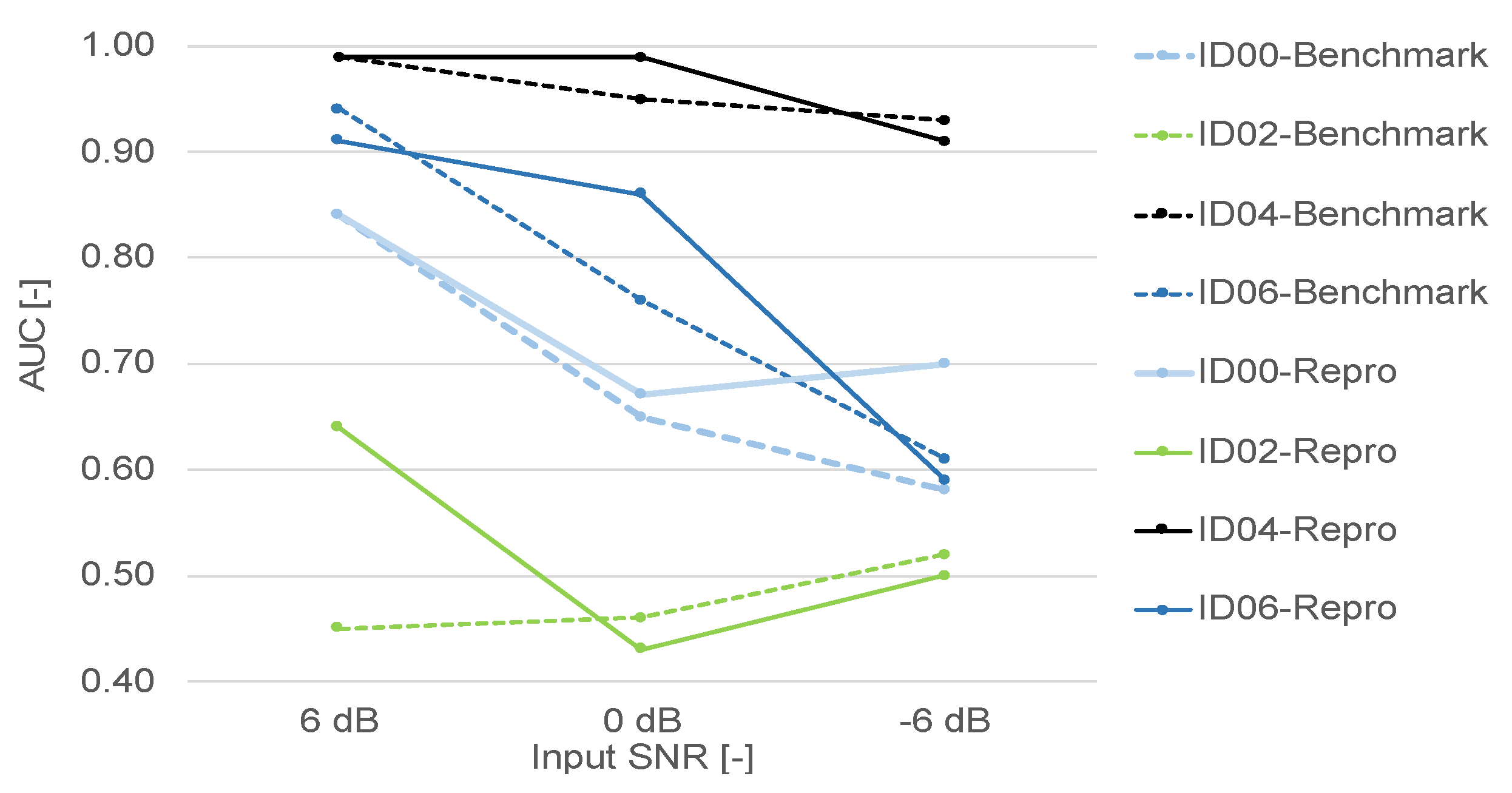
| ID00 | 0.84 | 0.65 | 0.58 | 0.84 | 0.67 | 0.70 |
| ID02 | 0.45 | 0.46 | 0.52 | 0.64 | 0.43 | 0.50 |
| ID04 | 0.99 | 0.95 | 0.93 | 0.99 | 0.99 | 0.91 |
| ID06 | 0.94 | 0.76 | 0.61 | 0.91 | 0.86 | 0.59 |
| Feature Dimensions | Performance Measure | Input SNR | ||
|---|---|---|---|---|
| 6 dB | 0 dB | −6 dB | ||
| 64 × 313 | Accuracy of Normal Condition Data | 0.91 | 0.93 | 0.96 |
| Accuracy of Anomalous Condition Data | 0.78 | 0.40 | 0.58 | |
| 320 | Accuracy of Normal Condition Data | 0.96 | 0.88 | 0.93 |
| Accuracy of Anomalous Condition Data | 0.68 | 0.42 | 0.56 | |
| Model ID | Input SNR | ||
|---|---|---|---|
| 6 dB | 0 dB | −6 dB | |
| ID06 | 0.9537 | TBA | 0.5941 |
| Model ID | Input SNR | ||
|---|---|---|---|
| 6 dB | 6 dB | −6 dB | |
| ID06 | 0.44 | 0.46 | 0.41 |
| Pre-Processing | Loss Function | AUC |
|---|---|---|
| Raw (unprocessed) | MSE | 0.7633 ± 0.0239 (Baseline) |
| MSE MSE with L2 Regularization | 0.7644 ± 0.0165 0.7909 ± 0.0192 | |
| KF | MSE | 0.7764 ± 0.0250 |
| MSE with L2 Regularization | 0.7898 ± 0.0200 | |
| UKF | MSE | 0.7644 ± 0.0165 |
| MSE with L2 Regularization | 0.7909 ± 0.0192 |
| Model ID | Input SNR [36] | Input SNR (This Paper) | ||||
|---|---|---|---|---|---|---|
| 6 dB | 0 dB | −6 dB | 6 dB | 0 dB | −6 dB | |
| ID00 | 0.84 | 0.65 | 0.58 | 0.8212 | 0.6792 | 0.6741 |
| ID02 | 0.45 | 0.46 | 0.52 | 0.5938 | 0.5576 | 0.5293 |
| ID04 | 0.99 | 0.95 | 0.93 | 0.9979 | 0.9753 | 0.9226 |
| ID06 | 0.94 | 0.76 | 0.61 | 0.9281 | 0.7854 | 0.6518 |
Publisher’s Note: MDPI stays neutral with regard to jurisdictional claims in published maps and institutional affiliations. |
© 2021 by the authors. Licensee MDPI, Basel, Switzerland. This article is an open access article distributed under the terms and conditions of the Creative Commons Attribution (CC BY) license (https://creativecommons.org/licenses/by/4.0/).
Share and Cite
Tagawa, Y.; Maskeliūnas, R.; Damaševičius, R. Acoustic Anomaly Detection of Mechanical Failures in Noisy Real-Life Factory Environments. Electronics 2021, 10, 2329. https://doi.org/10.3390/electronics10192329
Tagawa Y, Maskeliūnas R, Damaševičius R. Acoustic Anomaly Detection of Mechanical Failures in Noisy Real-Life Factory Environments. Electronics. 2021; 10(19):2329. https://doi.org/10.3390/electronics10192329
Chicago/Turabian StyleTagawa, Yuki, Rytis Maskeliūnas, and Robertas Damaševičius. 2021. "Acoustic Anomaly Detection of Mechanical Failures in Noisy Real-Life Factory Environments" Electronics 10, no. 19: 2329. https://doi.org/10.3390/electronics10192329
APA StyleTagawa, Y., Maskeliūnas, R., & Damaševičius, R. (2021). Acoustic Anomaly Detection of Mechanical Failures in Noisy Real-Life Factory Environments. Electronics, 10(19), 2329. https://doi.org/10.3390/electronics10192329