Performance Margin and Reliability Modeling Method for Multi-Level Redundant System

Abstract

This study proposes a multi-level performance margin modeling and belief reliability framework for redundant systems. Starting from system performance, a “performance–margin–reliability” linkage is established by defining the performance and margin of multi-level redundant systems and deriving performance, margin, and metric equations that account for failures. For complex redundant systems, a hierarchical Behavior Interaction Priority (BIP) modeling approach is developed to explicitly represent the normal and failure states of atomic component models. The effects of redundant components on the overall system are transformed into variations of performance parameters, enabling quantitative analysis of redundancy mechanisms. This paper proposes a boundary search algorithm for pruning optimization, which breaks through the computational bottleneck of non-analytic threshold sets in high-dimensional topological spaces. A case study on a power supply system with multi-level structural redundancy is conducted. Based on the proposed method, a performance-margin model of the redundant power supply system is constructed, critical states are analyzed, and system reliability is calculated. The results verify the effectiveness of the proposed margin-equation formulation and solution algorithm, offering practical guidance for reliability design of redundant systems.

1. Introduction

As complex systems with high reliability, redundant systems are widely used in aerospace, Internet communication, nuclear energy safety and other fields, especially in electronic systems in key fields. The design of multi-level redundant system is often used. The failure behavior of redundant systems is diverse and the state changes are complex. Therefore, the reliability modeling and analysis of redundant systems have always been a key and active research topic in the field of reliability system engineering. Scientifically and reasonably predicting and evaluating the reliability performance of redundant systems is the foundation for achieving reliable design, risk avoidance, and developing maintenance and support strategies for electronic systems.

The modeling of redundant systems has long been a central research focus in the field of reliability engineering. Existing modeling approaches include traditional methods such as reliability block diagrams (RBD) [1], fault trees [2], Petri nets [3,4], and Markov processes [5]. In recent years, methods based on binary decision diagrams (BDD) [6] and universal generating functions (UGF) [7] have also attracted increasing attention.

The reliability block diagram method represents the most fundamental modeling approach in reliability analysis and is suitable for relatively simple redundant-system modeling problems. Benabid et al. [1] employed the RBD method to evaluate the reliability of a redundant power supply system and compared the results with those obtained using fault tree analysis. Ahmadi et al. [8] conducted a reliability assessment of various redundancy strategies for modular multi-level converters.

Traditional static failure-tree logic gates cannot effectively represent the temporal dynamics of redundant systems. To address this limitation, researchers have developed dynamic fault trees [9], state/event fault trees [2] and fuzzy fault trees [10]. The solution of such complex fault trees often requires transformation into Markov chains [5] or Monte Carlo simulations [11].

The transitions between states in a redundant system can be regarded as a stochastic process. When the state transition is assumed to depend only on the current state and not on the previous ones, the process exhibits the Markov property. Consequently, the Markov processes are frequently employed for modeling redundant systems. Zhong et al. [12] incorporated system state duration into a regenerative-point method and a semi-Markov process to construct a cold-standby system model, addressing the problem of optimal preventive maintenance strategies. Fathizadeh et al. [13] proposed a model for a cold-standby system comprising a single server and two identical units with an imperfect switch, based on a matrix renewal function and a semi-Markov process. However, when applied to complex systems, the Markov modeling approach suffers from a rapid increase in computational complexity as the number of components and states grows, leading to the well-known state-space explosion problem.

Petri nets are capable of describing the dynamic characteristics of complex discrete-event systems and are commonly used for state-transition modeling of redundant systems. Ereau et al. [3] elaborated on the process of modeling redundant systems using Petri nets. Zeng et al. [14] employed Petri nets to conduct quantitative analyses of failure dependencies and common-cause failures within redundant systems. Chen and Zhang [4] proposed a novel emergency supply chain stress evolution modeling methodology based on stochastic Petri nets and corresponding isomorphic Markov chain model. As an information-flow model, however, the Petri net cannot directly support analytical computation; instead, it requires auxiliary analytical or simulation-based methods for quantitative evaluation.

In recent years, decision diagram–based modeling methods have gained widespread attention in redundant-system analysis due to their advantages in handling temporal logic, compatibility with multi-level redundant system, and immunity to the combinatorial explosion problem during computation. For example, Zhai et al. [6] utilized a generalized binary decision diagram to model the reliability of warm-standby systems. For k/n warm-standby systems with component lifetimes following arbitrary distributions, Tannous et al. [15] proposed a system reliability evaluation method based on sequential binary decision diagrams. Jia et al. [16] applied a multi-state multi-valued decision diagram modeling approach to address reliability assessment problems for demand-oriented warm-standby systems in which component degradation follows arbitrary distributions. Mo and Xing [17] integrated binary decision diagrams with multi-valued decision diagrams to perform reliability analysis of warm-standby systems. Yeh et al. [18] proposed an improved d-MP method based on a multistate flow network to study the reliability of logistics delivery in trucks driving on two types of roads under constraints.

The Universal Generating Function (UGF) is essentially a probabilistic computation method that enables the combination of discrete random variables, thereby addressing the problem of state-combination probability calculation in redundant systems. Owing to its simplicity and computational efficiency, the UGF approach has been widely applied to reliability modeling of multi-level redundant system. For active-standby redundant systems, Wang et al. [7] employed the interval UGF method and a discrete approximation approach to solve the reliability optimization problem of heterogeneous cold-standby systems. Levitin et al. [19] integrated the UGF method with the reliability block diagram approach to determine the performance of heterogeneous warm-standby systems under discrete-state and continuous-time processes. Furthermore, they proposed a UGF-based method for obtaining the demand satisfaction probability, which effectively addressed the optimal component allocation and sequencing problem in warm-standby systems [20].

Most existing reliability modeling approaches for redundant systems focus on failure relationships, emphasizing component lifetime distributions or failure rates to establish the link between reliability and failure probability. However, these conventional methods encounter fundamental limitations when applied to complex multi-level architectures: they often suffer from computational state-space explosion, rely on invalid component independence assumptions that overlook dynamic coupling, and, most critically, restrict analysis to binary logical states, thereby failing to capture the ‘Performance Margin’—the quantifiable distance to functional thresholds. Yet, reliability is fundamentally defined as the ability of a system to perform its intended function under specified conditions. This capability is intrinsically evaluated by determining whether system performance satisfies a given threshold; failures, in essence, influence reliability precisely through their impact on this performance [21].

In 2013, Professor Kang [22] proposed the belief reliability approach, which quantifies the influence of specified conditions on system performance through performance equations, describes performance degradation over time through degradation equations, derives performance margins using margin equations to represent whether system performance meets functional requirements, and evaluates the uncertainty of performance margins through metric equations to measure system reliability. The belief reliability method has been widely applied in the reliability modeling of systems. The theory of belief reliability, based on the uncertain maximum likelihood method and the uncertain variational inference algorithm, solves the problem of insufficient data in reliability analysis of two-stage degradation modeling [23]. In order to describe the state transition process of multi-state deteriorating systems under the effect of epistemic uncertainty, a mathematical model called uncertain state transition chain is proposed based on belief reliability [24]. The arithmetic Liu process based on belief reliability is used to model the uncertain performance degradation process of the components in the feedback control system [25]. The hybrid uncertainty of dependent competing failure process system is analyzed and quantified with chance theory based on belief reliability to solve the quantification problem of mixed uncertainty in these systems [26]. These methods have been demonstrated to be a more scientific and comprehensive reliability modeling framework. Within the belief reliability modeling theory, the margin equation defines the system’s performance margin as a distance function between system performance and its threshold. The accuracy of the margin equation directly affects the computation of the metric equation and the overall reliability assessment, making it a critical component of reliability analysis.

A multi-level structure consists of a hierarchical architecture where redundancy strategies are applied at distinct system levels. Unlike single-level designs, this configuration introduces complex cross-level state dependencies. Static methods struggle to represent dynamic transitions between levels, and dynamic methods often suffer from severe state-space explosion. More importantly, modeling the coupling between failure behaviors and performance is practically necessary for high-reliability applications. A system may remain logically functional after a partial failure, yet its performance can degrade significantly, shrinking the safety margin toward a critical threshold. Ignoring this coupling leads to overly optimistic reliability assessments. It fails to identify “grey states” where the system is topologically intact but performance-wise borderline.

However, traditional methodologies face critical challenges in accurately capturing this linkage for multi-level redundant systems. Static tools like RBD and FT fail to model internal failure dependencies or dynamic temporal behaviors, while Markov processes and Petri nets are hindered by state-space explosion or low computational efficiency. Furthermore, decision diagrams and UGF depend heavily on prior statistical data, often overlooking the physical connections between failures and the influence of external operating conditions. To bridge these modeling gaps and quantitatively evaluate performance margins under specified conditions, this study introduces a hierarchical framework based on Behavior Interaction Priority (BIP), which unifies physical laws and logical rules to enable a precise ‘Performance–Margin–Reliability’ linkage.

To address these gaps, this study proposes a hierarchical framework based on Behavior Interaction Priority (BIP). The effectiveness of the proposed approach stems from three core mechanisms: (1) Complexity Reduction: Hierarchical BIP modeling utilizes equivalent connectors to flatten cross-level interactions, representing complex behaviors with minimal layers to bypass the state-space explosion inherent in traditional dynamic methods. (2) Failure-Performance Coupling: The ‘Performance–Margin–Reliability’ linkage maps discrete failure transitions within atomic components directly to continuous performance parameter variations. (3) Analytical Support: A pruning-optimized boundary search algorithm provides a rigorous numerical solution for high-dimensional, non-analytic threshold sets, enabling precise reliability quantification where simple analytical expressions are unavailable.

The innovations of this study are reflected in the following aspects:

(1)

Presents the definitions of performance and margin for multi-level redundant system, together with the basic workflow of performance margin modeling for redundant systems, thereby laying the foundation for belief reliability modeling of redundant systems.

(2)

Investigates a BIP-based modeling method for redundant-system performance that considers system failure behavior coupling. The failure behaviors introduced by adding redundant components to the original system are incorporated into the performance margin modeling, and—under the coupling between system behavior and redundant components—the system’s margin equation is established.

(3)

Addressing the issue that the performance range of complex multi-level redundant systems forms a high-dimensional topological set that is difficult to describe with simple functions, a depth-first search method with pruning optimization is adopted to rapidly obtain numerical solutions for the set boundary (requirement thresholds), thereby avoiding the excessive computational burden of exhaustive enumeration.

The remainder of this paper is organized as follows: Section 2 presents the concepts of performance and margin for multi-level redundant systems and provides the margin expressions and modeling procedure for redundant systems. Section 3 introduces the basic principles of the BIP modeling method, proposes a multi-level redundant system BIP modeling approach that considers the influence of failure behavior coupling, and develops a boundary search algorithm for solving the margin equation. Section 4 takes a multi-level redundant power-supply system as an example to demonstrate the implementation process and results of the proposed modeling method. Section 5 summarizes the paper and discusses potential directions for future research.

2. Performance and Margin Modeling of Multi-Level Redundant System

2.1. Definition of Performance and Margin in Redundant Systems

Professor Rui Kang [24] proposed three fundamental principles of reliability science within the framework of belief reliability theory: the margin reliability principle, the degradation eternity principle, and the uncertainty principle. He further pointed out that the reliability model of a system can be constructed using four fundamental equations—the performance equation, the degradation equation, the margin equation, and the metric equation—among which the performance degradation equation is expressed as follows: [22]

$$P=f_{\overrightarrow{t}=0}(X,Y,t)$$

(1)

where X denotes the internal variable, Y denotes the external variable, t represents reversible time, P represents the vector of system performance parameters (hereinafter referred to as performance parameters), and $f_{\overrightarrow{t}=0}(\cdot )$ a denotes the functional relationship among the aforementioned variables. Equation (1) serves as the general form of the performance degradation equation for various types of systems. For redundant systems, by considering both the failure state and the system state, the performance degradation equation can be expressed as:

$$P(\delta )=\left\{\begin{array}{ll}{F}_0(X,Y,t)\hfill & \delta =0\hfill \\ F_{\delta }(X(\delta ),Y(\delta ),t)\hfill & 0<\delta \le {\delta }_m\hfill \end{array}\right.$$

(2)

In this equation, $\delta$ represents the index of the current state of the redundant system. The system’s state is defined by the combination of failure conditions of its functional components, where each unique combination corresponds to a specific failure configuration. ${\delta }_m$ represents the maximum number of failures that the system can tolerate before it is considered to have completely failed. Thus, $\delta$ tracks the current failure status of the system, while ${\delta }_m$ defines the system’s failure tolerance threshold. When $\delta =0$, the system is in the normal operating state, meaning no failure has occurred. When $0<\delta \le {\delta }_m$, the system is in a failure state, with δ indicating the number of failures that have occurred. For convenience, the representative index of the state in which the redundant system operates normally is denoted as $1-{\delta }_m$. $F_0$ represents the performance equation of the system when no failure has occurred, hereinafter referred to as the performance equation of the initial state of the redundant system. $F_{\delta }$ represents the performance equation of the system after recovery or reconfiguration; if reconfiguration is not considered, then $F_0$ remains equivalent to $F_{\delta }$. It can thus be seen that the performance equation describes the physical law governing system performance, encompassing the dynamic evolutionary behavior of the system caused by failures.

It is assumed that, within the n-dimensional normalized margin space $R^{n^{*}}$ of the redundant system, there exist demand threshold points $P_{th}\in \partial A$, $\forall \delta \le {\delta }_m$, and the performance parameter $P(\delta )$ serves as the unique solution to the performance equation, as illustrated in Figure 1. In this case, the system’s performance parameter is a fixed value—for example, the output voltage of the power supply in electronic equipment. This type of performance parameter does not vary with changes in user demand.

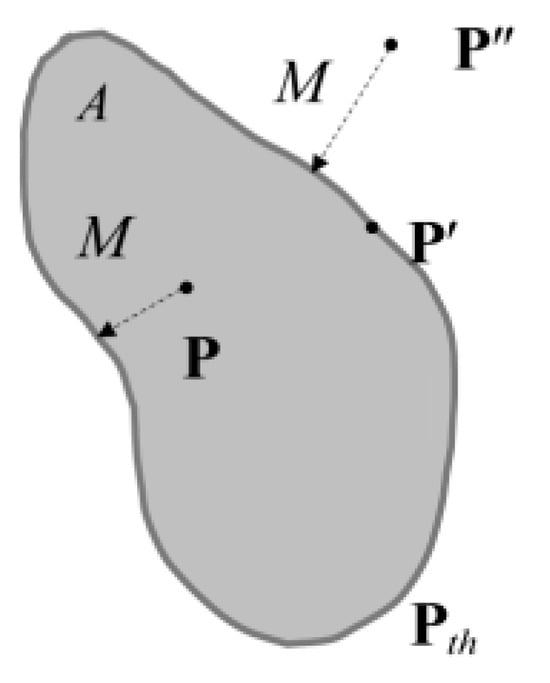
Figure 1. Performance margin diagram of redundant system.

In Figure 1, the dashed arrow represents the margin M, A represents the range of performance parameters that satisfy the functional requirements of the system, while ${\mathbf{P}}_{\mathbf{t}\mathbf{h}}$ denotes the demand threshold. The boundary of the performance index range is a set composed of these demand thresholds. For each point $\forall \delta \le {\delta }_m$, the performance equation has unique solutions $\mathbf{P}$, ${\mathbf{P}}^{\mathbf{\prime }}$, and ${\mathbf{P}}^{\mathbf{″}}$, respectively. For a redundant system, system reliability implies that, for all $\forall \delta \le {\delta }_m$, the solutions of the performance equation must satisfy the functional requirements.

The performance of a redundant system is related to the internal failures that occur within it and can be characterized by the representative failure index $\delta$, which indicates the current functional state combination of the system. When $\forall \delta \le {\delta }_m$, the shortest distance $P(\delta )$ between the performance parameter $M(\delta )$ and its corresponding demand threshold can be used to describe the reliability performance of the redundant system. Accordingly, the performance margin of the redundant system is defined as the expected value of the system’s performance margin $\forall \delta \le {\delta }_m$ over all system states $M(\delta )$.

Without considering system recovery or reconfiguration after failures, the expression of the performance margin $M(\delta )$ is given as follows:

$$M(\delta )=\left\{\begin{array}{ll}\underset{P_{th}\in \partial A_{th}}{\min }{\pi }_1(F_0(X,Y,t),P_{th}){‖F_0(X,Y,t)-P_{th}‖}_2\hfill & \delta =0\hfill \\ \underset{th\in \partial A_{th}}{\min }{\pi }_1(F_0(X(\delta ),Y,t),P_{th}){‖F_0(X(\delta ),Y,t)-P_{th}‖}_2\hfill & 0<\delta \le {\delta }_m\hfill \end{array}\right.$$

(3)

where ${\pi }_1(\cdot )$ denotes the indicator function, $A_{th}$ represents the range of performance parameters that satisfy the functional requirements of the system, and $\partial A_{th}$ represents the boundary of the performance index range $A_{th}$, corresponding to the demand threshold. The value of the indicator function is 1 if and only if C and C both satisfy the specified constraint relationship; otherwise, it is 0.

Let the probability density function of the system being in different performance state combinations be denoted as $f(\delta )$, then the performance margin equation of the redundant system considering uncertainty can be expressed as:

$$M_{re}={\displaystyle {\int }_0^{{\delta }_m}f}(\delta )M(\delta )d\delta$$

(4)

where ${\delta }_m$ represents the maximum representative index of allowable failures in the redundant system. Specifically, when $\delta$ is a discrete variable, Equation (4) can be reduced to a discrete form:

$$M_{re}={\displaystyle \sum _{\delta =0}^{{\delta }_m}f}(\delta )M(\delta )$$

(5)

The system reliability is defined as the probability that the performance margin is greater than zero, i.e., the metric equation is expressed as:

$$R=c\{M_{re}(\delta )>0\}$$

(6)

where $R$ denotes the belief reliability, and $c\{\cdot \}$ represents the mathematical measure used to quantify uncertainty, such as a probability measure.

2.2. Basic Process of Performance Margin Modeling for Complex Redundant Systems

Equation (3) represents the general form of the margin equation for redundant systems. For complex multi-level redundant systems, the margin cannot be expressed in a simple equation form. Instead, an approach involving the construction of a surrogate multi-level diagram model can be used. The process for constructing the margin equation for complex redundant systems is shown in the flow diagram in Figure 2. (a) is the conceptual relationship between belief reliability, performance margin, and the hierarchical BIP model. (b) is the basic process for establishing the margin equation of redundant systems.

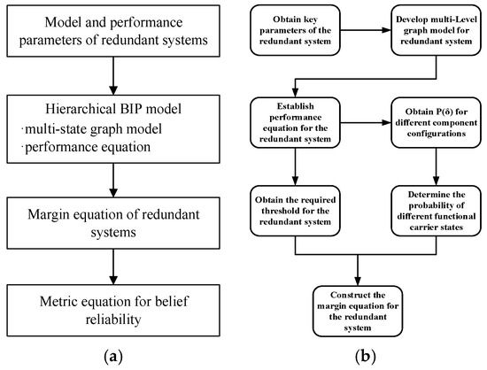
Figure 2. Basic process for establishing the margin equation of redundant systems. (a) The conceptual relationship. (b) Establishing the margin equation.

(1)

By collecting information on the design, structure, functions, and other aspects of the redundant system, key performance parameters of the system are obtained using functional, performance, and margin analysis methods. Based on this, the hierarchical structure and information for modeling the redundant system are organized.

(2)

Using the information obtained in step 1, a multi-state graph model of the redundant system is constructed (e.g., the BIP model described later). The BIP model serves as a surrogate form for the redundant system’s performance equation. During the construction of the BIP model, the first step is to identify the internal and external parameters of the redundant system that need to be analyzed, followed by the selection of the necessary BIP components and modeling methods.

(3)

The system’s performance equation is obtained based on the BIP model. If there are correlations between different key performance parameters, decoupling must be performed first to ensure independent performance equations are derived. By simulating the BIP model, the values of the system performance parameters under the given internal and external parameters can be obtained.

(4)

The demand thresholds of the redundant system are determined, completing the construction of the system’s margin equation. All constraints are integrated, and a functional expression satisfying the demand thresholds is provided. This allows for the determination of the probabilities of the system being in different functional carrier states, thus obtaining the distribution of the system, which is substituted into Equation (4) or (5). Finally, the belief reliability is calculated using Equation (6).

3. BIP Modeling Method for Performance Margin of Redundant Systems

3.1. BIP Modeling Method

The BIP model mentioned in Figure 2, is a formal modeling framework proposed by the Verimag Laboratory in France (founded by Turing Award winner Joseph Sifakis [27]). It is primarily used for the design and verification of complex systems. The core idea of this model is to describe system dynamics through the interactions between components and use a priority mechanism to address concurrency control issues [28].

The BIP model consists of three layers: The bottom layer describes the behavior of atomic components through an extended labeled transition system. The middle layer expresses the interactions between components via connectors, which can be defined on any number of ports. The types of connectors include rendezvous (strong synchronization) and broadcast. The top layer defines interaction priority rules that are used to schedule the sequence of interactions in the bottom layer. These priorities describe the system’s scheduling strategy and allow for the implementation of complex logical relationships.

The atomic component consists of a set of ports (Ports), local variables (Variable), a set of states (States), and several transitions (Transitions). Figure 3 shows the general structure of an atomic component, which primarily includes the port set, state set, variable set, and the set of transitions corresponding to the modeling computation steps.

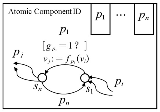
Figure 3. Atomic component structure diagram.

In Figure 3, the ports of the atomic component are generally denoted by $\mathbb{P}=\{p_1,p_2,\dots ,p_n\}$. Ports are operation names used for synchronizing with other components. The state set is represented by $\mathbb{S}=\{s_1,s_2,\dots ,s_n\}$, where the control state indicates the position where the component is waiting for synchronization. The variable set is denoted by $\mathbb{V}=\{v_1,v_2,\dots ,v_n\}$, used to represent the numerical values of variables in the model. The set of transitions consists of multiple transitions. A transition from state $s_i$ to state $s_j$ is represented by the $\left(s_i,p,g_p,f_p,s_j\right)$ tuple, where $p$ denotes the port related to this transition, which can exchange data with other components. $g_p$ represents the guard condition for the transition, specifying the conditions under which the transition can occur, typically evaluated using a Boolean variable. $f_p$ represents the action to be executed when the transition occurs; this action can execute a function on the variable set.

3.2. BIP Modeling Method for Multi-Level Redundant Systems

In the BIP model of a redundant system, each atomic component can represent either a system-level component or a subsystem-level unit. For atomic components representing system-level components, there must be two or more states, with one state being a failure state and the remaining states representing normal or intermediate states. The corresponding set of transitions must include at least one transition whose endpoint is the failure state. The execution action of this transition can represent the performance equation and the dynamic evolution behavior of the system caused by failures. The guard condition for the transition leading to failure represents the failure criterion of the system component at the unit level.

For multi-level redundant systems, the system performance equation based on BIP is constructed by modeling from the lowest layer to the higher layers. The lowest-level components can be represented by BIP atomic components, which describe behavior and interaction. At higher levels, BIP atomic components can describe the redundancy rules at the subsystem level. For the entire system, it is necessary to combine the lower-level BIP atomic components with the higher-level BIP atomic components. Here, we introduce BIP composite components to represent the BIP model for such multi-level systems. The composite component model has ports for interacting with the external environment, and its internal structure consists of interactions between lower-level atomic components, as shown in Figure 4.

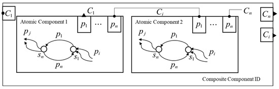
Figure 4. Construction of BIP model composite component.

The BIP model of a system with multi-level redundancy can achieve component-level reuse through the addition of ports and interactions. However, due to the complexity of the system’s multiple level, it becomes difficult to implement the model programmatically. To address this, the logical relationships need to be simplified to describe the global impact of each component’s behavior on the system behavior using the fewest system layers. By using equivalent connectors, the interactions across different levels in the multi-level BIP model can be flattened, i.e., the internal interactions within composite components and the external interactions are mapped to the same level. The three types of connectors shown in Figure 5 are equivalent [29].

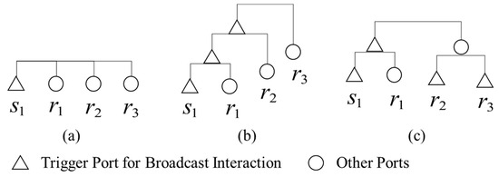
Figure 5. Equivalent transformation of interactions between multi-level and single-level BIP models. (a) Single-level interaction (b) Three-level interaction (c) Two-level interaction.

The performance BIP model of a redundant system can adopt a multi-level BIP model, where the atomic component model includes both normal and failure states. This allows for the consideration of the impact of system failure behavior on the performance of redundant components. The relationship between redundant components represents the new component behavior generated by adding redundant system components to the original system. There is an interaction between system behavior and the redundant component relationships, and the effects of this interaction will be reflected in the changes to the system performance parameters.

3.3. Boundary Search Algorithm for Margin Equation

Based on the characteristics of the margin equation for redundant systems, constructing the margin equation requires obtaining the range A of performance parameters that satisfy the functional requirements of the system, along with their threshold $P_{th}$ (as shown in Figure 1). For complex systems, the range of performance parameters needs to be represented by a set in a high-dimensional topological space, and the boundary of this set corresponds to the threshold. Since it is difficult to describe the boundary of a high-dimensional topological space set using a function, the most straightforward method is to use exhaustive enumeration to obtain the numerical solution of the boundary. However, this approach is computationally expensive and inefficient.

This section proposes a depth-first search method with pruning optimization to quickly obtain the numerical solution for the boundary of the high-dimensional topological space. The core idea is to search the boundary and identify as many points as possible to replace the boundary curve, thereby obtaining the required threshold. To fully explain the algorithm’s process, the following definitions are provided.

Definition 1. 

Let there be a topological space  $(R^n,{\mathcal{T}}_{p_0^n})$ and a set  $x\in R^n$. Using  $x$ as the origin and a step size of  $\lambda$ , the topological space is discretized into a set of evenly spaced points. The resulting new set of points  $U_{x-\lambda }$ is called the gridding of the topological space  $(R^n,{\mathcal{T}}_{p_0^n})$.

Definition 2. 

Let there be a point set  $R^{n^{*}}$ in the normalized margin space  $U_x$,  where the elements in the set satisfy the rule  ${\mathbb{F}}_U$.  By gridding  $R^{n^{*}}$ and using a Boolean value  $b_u$ to distinguish between the points that satisfy rule  ${\mathbb{F}}_U$ and those that do not, a tuple  $\left([x_1,\dots ,x_n],b_u\right)$ is formed. The set composed of these tuples  $ℍ$ is referred to as the grayscale of the normalized margin space.

A complete example of the gridding and grayscale process in a three-dimensional normalized margin space is shown in Figure 6.

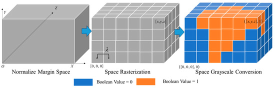
Figure 6. Gridding and Grayscale process of the normalized margin space.

Through the processes of gridding and grayscale transformation, the high-dimensional space can be represented by a discrete set of points, with the original boundary curve approximated by connecting boundary points. The accuracy of this approximation depends on the gridding step size. Based on the grayscale transformation of the space, it can be observed that the boundary points still satisfy the necessary and sufficient conditions for boundary points in the topological space. In this study, a depth-first search method is employed to identify the boundary points, while pruning optimization is applied to terminate the search early for neighboring points of certain boundary points. The principle of this method is illustrated in Figure 7.

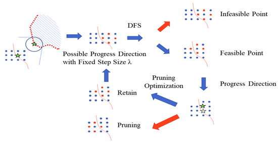
Figure 7. Schematic diagram of the domain boundary search algorithm.

The forward direction and termination conditions of the depth-first search follow the rules below:

(1)

The forward search direction consists of the $3^n-1$ adjacent searchable points of the current point. For example, if the current point is $\left(0,0\right)$, the adjacent searchable points are $\left(1,0\right)$, $\left(0,1\right)$, $\left(1,1\right)$, $\left(-1,0\right)$, $\left(0,-1\right)$, $\left(-1,-1\right)$, $\left(-1,1\right)$ and $\left(1,-1\right)$

(2)

The termination condition is that the Boolean value of the current point equals 1, and within an open ball of radius ${\gamma }_a({\gamma }_a>\lambda )$ centered at the current point $a$, there exist points $B(\mathit{a};{\gamma }_a)=\left\{ \mathit{x}\in {\mathbf{R}}^n\mid {\rho }^n(\mathbf{x},\mathbf{a})<{\gamma }_a\right\}$ with Boolean values of both 1 and 0. In this case, the search continues; otherwise, the search terminates and backtracks to the previous search point.

It is worth noting that the radius of the open ball in the termination condition should not be excessively large, as an overly large radius will always include points with Boolean values of both 1 and 0. Based on empirical experience, the maximum selectable radius should not exceed $\sqrt{9n}\lambda$.

To improve the search speed of the depth-first search algorithm, the following pruning optimization rules are adopted:

(1)

If only one-third or fewer of the adjacent searchable points of the current point do not satisfy the termination condition, then these adjacent points will not be searched. For example, if the current point is $\left(0,0\right)$ and only $\left(1,1\right)$ among its adjacent searchable points can continue the search, while the remaining points satisfy the termination condition, then these remaining adjacent points $\left(1,1\right)$ will not be considered as the next current point in the subsequent search step.

(2)

If the Boolean value of the current point is 0, none of its adjacent searchable points will be searched.

(3)

If three-fourths or more of the adjacent searchable points of the current point do not satisfy the termination condition, then the adjacent points of the current point will also not be searched. For example, if the current point is $\left(0,0\right)$ and among its adjacent searchable points $\left(1,0\right)$, $\left(0,1\right)$, $\left(1,1\right)$, $\left(-1,0\right)$, $\left(0,-1\right)$, $\left(-1,-1\right)$, $\left(-1,1\right)$ and $\left(1,-1\right)$ can continue the search, then the remaining adjacent searchable points will not be considered as the next current points.

Based on the above definitions and rules, the process of the proposed domain boundary search algorithm is shown in Figure 8.

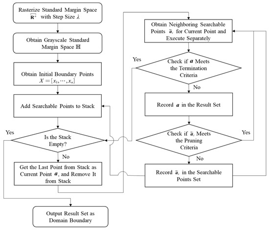
Figure 8. Flowchart of the boundary search algorithm.

3.4. System Reliability Calculation Method

To solve the margin equation of a redundant system, it is first necessary to obtain the shortest distance between the performance parameters and the demand thresholds under each system state. Then, the margin is determined based on the probability of each system state, followed by the calculation of system reliability. The main steps are as follows:

(1)

Generate the set of system states in which the redundant system can operate normally.

(2)

Use the boundary search algorithm to obtain the demand threshold $\partial A_{th}$.

(3)

Based on the system performance equation, calculate $F_0(X,Y,t)$ and $F_0(X(\delta ),Y,t)$; for a given $\delta$, iterate over each ${\mathbf{P}}_{th}\in \partial A_{th}$ to compute the corresponding ${\pi }_1\left(F_0(X(\delta ),Y,t),P_{th}\right){‖F_0(X(\delta ),Y,t)-P_{th}‖}_2$ and take the minimum value, with $\delta$ serving as $M\left(\delta \right)$ under the given condition.

(4)

According to the obtained $f\left(\delta \right)$, select Equation (4) or (5) as appropriate to compute $M_{re}$, and then calculate the system reliability using Equation (6).

4. Case Analysis

4.1. Case Introduction

The power supply system of a certain industrial control device adopts a multi-level redundant system design as shown in Figure 9. The battery simultaneously powers two chargers, each consisting of four charging modules. Two of the modules serve as the primary working components, while the other two are used for hot backup. The two chargers are connected in parallel for redundancy.

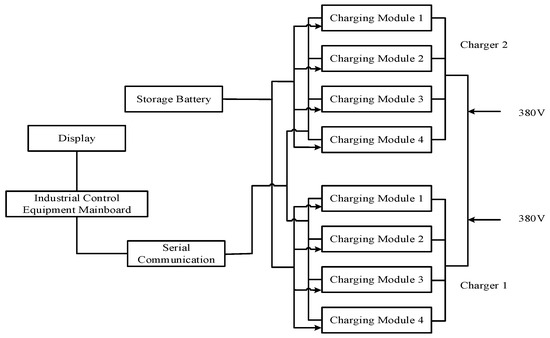
Figure 9. Power supply system structure diagram.

The function of the power supply system is to provide a fixed current output by the charging modules. Failure detection occurs when none of the chargers can meet the required output current. Each charging module is controlled by the device’s mainboard through serial communication, which enables switching between failure and backup modules, as well as the selection and matching of primary working modules and charger output control. The control logic of the device mainboard is as follows: the mainboard monitors the status of each working module. When all charging modules within the same charger are operating normally, the two modules with the highest total output current are selected as the primary modules, while the remaining modules serve as hot backups. When a primary module fails, the charging module with the highest output current among the backup modules is activated as the new primary module. In the two chargers, the charger with the highest output current is selected to supply power. Considering that the effective voltage supplied to the battery must not be too low, there are corresponding requirements for the equivalent internal resistance of the charging modules. Since the output current and the equivalent internal resistance of the charging modules are relatively independent performance parameters, the system’s performance is represented as a two-dimensional vector consisting of output current and equivalent internal resistance.

4.2. Power Supply System BIP Modeling

The first step is to establish the atomic components of the power supply system. Figure 10 illustrates the atomic component construction for a non-repairable single resistor in a parallel resistor configuration. This resistor has two states: $S_1$ represents the abnormal state, and $S_2$ represents the normal state. The operating state corresponds to a self-loop transition $P_2$. $P_1$ denotes an abnormal state caused by over-voltage disconnection or short-circuiting (denoted as $\epsilon =0$). The current flowing through the resistor is represented by $I=0$, while $p_3$ indicates an abnormal state caused by the short circuit. $\alpha =1$ is the short-circuit indicator. The input port in transmits the voltage signal to the resistor, and ports $P_1$, $P_2$, and $p_3$ transmit the state indicator signal and current signal to another parallel resistor and subsequent circuitry, respectively.

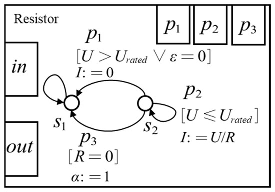
Figure 10. Atomic component construction of a single resistor in a parallel resistor configuration.

The atomic components are combined to form a multi-level BIP model. Figure 11 shows the multi-level BIP model of Charger 1.

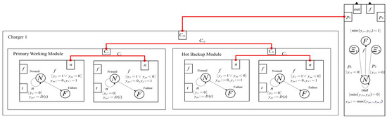
Figure 11. Multi-level BIP model of charger 1.

By applying simplification rules, the BIP model of the system is reduced, as shown in Figure 12.

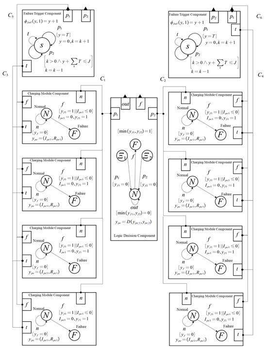
Figure 12. BIP model of the power supply system.

In the redundant system’s BIP model, two failure-triggering components are set up to act on the charging modules in Charger 1 and Charger 2, respectively. The $f$ ports of the four charging modules strongly interact with the failure output port $p_1$ of the failure-triggering components to ensure that failure information is synchronized across all components. The time progression of the failure-triggering components is strongly synchronized with the time progression of each component through port $t$. Each charging module component includes both normal and failure states. The normal state port $n$ connects to the logic decision component port via connectors $C_1$ and $C_2$, where the protective device of the connector judges the status of the charging modules within the charger and performs the action of selecting the charging module as the primary working module. $I_{pe\_1}$ and $I_{pe\_2}$ are assigned to the current outputs of Charger 1 and Charger 2 via the connectors, and their expression is as follows:

$$I_{pe\_1}=\underset{i\ne j}{\max }\left\{I_{i,1}+I_{j,1}\right\}$$

(7)

$$I_{pc\_2}=\underset{i\ne j}{\max }\left\{I_{i,2}+I_{j,2}\right\}$$

(8)

In this model, $I_{\mathrm{i},1}$ represents the output current capability of the charging module in Charger 1, while $i=1,2,3,4$ and $j=1,2,3,4$ represent the states of the logic decision component. The migration constraints for states $s_1$ and $s_2$ in the logic decision component are used to determine whether the charger itself can output normally. When both chargers can output normally, the system’s output current $I_{pe}$ is:

$$I_{pe}=\max \left\{I_{pe\_1},I_{pe\_2}\right\}$$

(9)

When at least one charger is functioning normally, the system state is considered a normal output state. In the case where both chargers fail, the system state transitions from the normal output state to a failure state. The output current during a charger failure is set to zero. The system’s equivalent resistance is calculated using the charger that is outputting and the primary working module’s charging module, based on the circuit’s equivalent resistance formula.

$$R_{pe}={\displaystyle \frac{R_{i,N}{R}_{j,N}}{R_{i,N}+R_{j,N}}}$$

(10)

In this model, $N$ represents the index of the charger with the largest output current from the two chargers, while $i$ and $j$ represent the indices of the two charging modules with the largest output currents in Charger $N$.

4.3. Performance Margin Equation of the Power Supply System

The current state of the redundant system can be represented by a tuple of the number of failures $N_{n-f}$ and the failure-bearing component index $N_{id-f}$. Each state of the redundant system is numbered and labeled as $\delta$, where $\delta =0$ represents the system state with no failures, and $\mathbf{X}\left(\delta \right)$ represents the changes in output current and equivalent internal resistance of the charging modules after a failure occurs. To simplify the description of the system’s performance equation, the physical laws governing the system’s performance at the initial moment (when no failures occur) and the system’s performance after a failure are derived. The simplified performance equation expression is obtained through the BIP model of the system:

$$P_{PS}=\left[\begin{array}{c}{I}_{pe}\\ R_{pe}\end{array}\right]=\left[\begin{array}{c}\underset{N=1,2}{\max }\left\{\underset{i\ne j}{\max }\left\{I_{i,N}(\delta )+I_{j,N}(\delta )\right\}{f}_y(N,\delta )\right\}\\ {\displaystyle \frac{R_{i(\delta ),N(\delta )}{R}_{j(\delta ),N(\delta )}}{R_{i(\delta ),N(\delta )}+R_{j(\delta ),N(\delta )}}}{f}_R(\delta )\end{array}\right]$$

(11)

where, $P_{PS}$ represents the performance parameter vector composed of the output current and equivalent internal resistance of the power supply system. ${\left[y_{pe},R_{pe}\right]}^T$ represents the performance parameters. $N\left(\delta \right)$ indicates the index of the charger selected under different redundant system states. $i\left(\delta \right)$ and $j\left(\delta \right)$ represent the indices of the two charging modules with the largest output currents in the selected charger $N\left(\delta \right)$. $f_y$ is the indicator function for output current; if the number of normally functioning charging modules in charger $\delta$ under the redundant system state represented by state number $N$ is fewer than 2, the function value is 0; otherwise, the function value is 1. $f_R$ represents the indicator function for equivalent internal resistance; if the output current of the redundant system state represented by state number $\delta$ is 0, the function value is $\infty$; otherwise, the function value is 1.

The performance margin equation of the power supply system is:

$$M=\underset{P_{PS}\in \partial A_{th}}{\min }{\pi }_1\left(P_{PS},P_{th}\right){‖P_{PS}-P_{th}‖}_2$$

(12)

4.4. Belief Reliability Analysis of the Power Supply System

The parameter table for each module in Charger 1 and Charger 2 is shown in Table 1. It includes the output current capability, equivalent internal resistance, and the failure detection criteria for the industrial control system.

Table 1. Parameter table for each module of charger 1 and charger 2.

Charger	Charging Module	Output Current (A)	Current Criterion	Equivalent Internal Resistance (mΩ)	Internal Resistance Criterion
Charger 1	1	57	<37.5 A	0.56	>1 mΩ
	2	50		0.44
	3	41		0.67
	4	38		0.80
Charger 2	1	56		0.41
	2	54		0.59
	3	49		0.65
	4	43		0.53

We first solve the performance equation, and the resulting system performance calculation is presented as a set of data points in Figure 13.

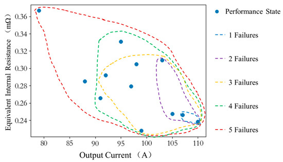
Figure 13. System performance vs. failure parameters in power supply charging.

In Figure 13, the horizontal axis represents the output current (A) and the vertical axis represents the equivalent internal resistance (mΩ). Colored dashed lines depict the boundaries of the system performance parameter set, which vary with failure conditions as the number of component failures increases from 1 to 5.

From Figure 13, we observe that as the number of failures in the failure parameters increases, the system performance shifts toward a lower output current and a higher equivalent internal resistance. Concurrently, the set of performance parameter points continually expands. Consequently, the solution to the system performance equation can be substituted by analyzing the change in the performance point set, which is influenced by the number of failures.

Specifically, when the number of system failures is six, these failure points significantly affect the system’s performance output. Crucially, the power supply system fails (system failure) when the number of system failures is greater than or equal to seven. The output current of the power supply system is constrained to be no less than 75 A and no more than 125 A. The relationship between the equivalent internal resistance limits and the output current is detailed in Table 2.

Table 2. Equivalent internal resistance limits vs. output current in power system.

Output Current Range (A)	Equivalent Internal Resistance Requirement (mΩ)
75 A ≤ I < 85A	Rr ≤ 0.40
85A ≤ I < 95A	Rr ≤ 0.37
95A ≤ I < 105A	Rr ≤ 0.36
105A ≤ I < 115A	Rr ≤ 0.33
115A ≤ I < 125A	Rr ≤ 0.30

The system’s Demand Threshold is governed by the failure criteria defined in Table 3 and the output current, which consequently dictates the rules satisfied by the points within the threshold. The set of points constituting this Demand Threshold is subsequently obtained using the Boundary Search Algorithm, as illustrated in Figure 14.

Table 3. Set of system states for normal power system operation. (Symbol “x”: arbitrary state of a functional carrier).

Serial Number ($\mathit{\delta }$)	System State	Output Current Capacity (A)	Serial Number ($\mathit{\delta }$)	System State	Output Current Capacity (A)
0	(x, x, x, x,1, 1, x, x)	110	7	(1, 0, 0, 1, 0, 0, x, x), (1, 0, 0, 1, x, 0, 0, 0), (1, 0, 0, 1, 0, x, 0, 0)	95
1	(1, 1, x, x, 0, x, x, x), (1, 1, x, x, x, 0, x, x)	107	8	(x, x, x, x, 0, 0, 1, 1), (0, x, x, x, 0, 0, 1, 1), (1, 0, 0, 0, 0, 0, 1, 1)	92
2	(0, x, x, x, 1, 0, 1, x), (x, 0, x, x, 1, 0, 1, x)	105	9	(0, 1, 1, x, 0, x, 0, 0), (0, 1, 1, x, x, 0, 0, 0), (0, 1, 1, x, 0, 0, 0, x), (0, 1, 1, x, 0, 0, x, 0)	91
3	(x, 0, x, x, 0, 1, 1, x), (0, x, x, x, 0, 1, 1, x)	103	10	(0, 1, 0, 1, 0, x, 0, 0), (0, 1, 0, 1, x, 0, 0, 0), (0, 1, 0, 1, 0, 0, 0, x), (0, 1, 0, 1, 0, 0, x, 0)	88
4	(0, x, x, x, 1, 0, 0, 1), (x, 0, x, x, 1, 0, 0, 1)	99	11	(0, 0, 1, 1, x, 0, 0, 0), (0, 0, 1, 1, 0, x, 0, 0), (0, 0, 1, 1, 0, 0, 0, x), (0, 0, 1, 1, 0, 0, x, 0)	79
6	(0, x, x, x, 0, 1, 0, 1), (1, 0, 0, 0, 0, 1, 0, 1)	97	\	\	\

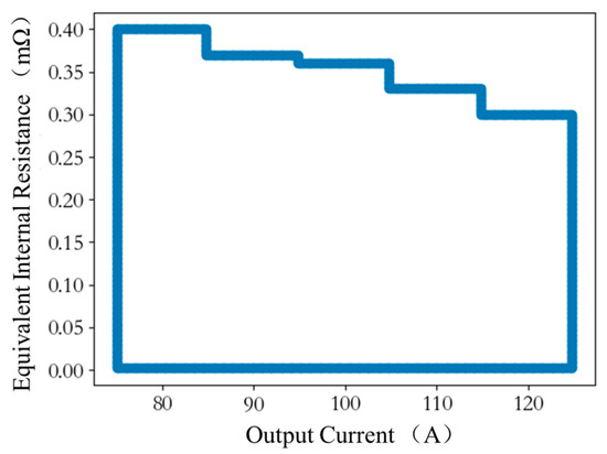
Figure 14. Set of demand threshold points for the power system.

As shown in Figure 14, where the axes and units are consistent with Figure 13, the algorithm solves for the numerical demand threshold set $P_{th}$. This boundary defines the acceptable region for system operation based on the combined constraints of output current and internal resistance.

Based on the configuration of the Redundant Power System, the set of system states enabling normal operation is generated. Specifically, the state of the redundant power system is represented by an octuple composed of the failure or normal status of the charging modules, where 0 and 1 denote the failure and normal status of the charging module’s functional carrier, respectively. A total of 239 system states capable of normal operation were obtained. These states are then consolidated based on the various combinations of operational chargers and charging modules serving as the system output, resulting in the categorized states presented in Table 3.

In Table 3, the symbol “x” denotes an arbitrary state, which can be either a failure or normal condition. The system states were consolidated into twelve distinct states differentiated by their output current capability. $M\left(\delta \right)$ and $f\left(\delta \right)$ are calculated and obtained separately using the Margin Solution Algorithm. It is evident that the performance margin for identical system state $M\left(\delta \right)$ possesses the same magnitude, and the calculation results for $M\left(\delta \right)$ are presented in Table 4.

Table 4. Performance margin for each system state of the power supply system.

System State $\mathit{\delta }$	Performance Margin $\mathit{M}\left(\mathit{\delta }\right)$	System State $\mathit{\delta }$	$\mathbf{Performance} \mathbf{Margin} \mathit{M}\left(\mathit{\delta }\right)$
0	0.091616	6	0.080803
1	0.08360	7	0.028905
2	0.08238	8	0.078051
3	0.050726	9	0.10441
4	0.132043	10	0.084880
5	0.054960	11	0.033311

Based on the failure criteria for charging modules provided in Table 1, the performance margin and belief reliability are calculated for the eight charging modules within the power system. Each charging module is characterized by two performance parameters—output current and equivalent internal resistance—along with their respective demand thresholds.

System uncertainty primarily originates from the parameter uncertainty of the charging modules, which is mainly introduced during the manufacturing process. The uncertainty of the power system’s margin is quantified using the normal distribution in probability theory. This analysis assumes that no failures exist in the industrial control equipment. The probability distributions for the parameters of the respective charging modules are given in Table 5.

Table 5. Probability distribution table of parameters for each charging module.

Charging Machine Serial Number	Output Current Capacity (A)	Equivalent Internal Resistance Requirement (mΩ)
Charger 1	N (57, 42)	N (0.56, 0.052)
	N (50, 5.22)	N (0.44, 0.022)
	N (41, 52)	N (0.67, 0.062)
	N (38, 6.12)	N (0.81, 0.052)
Charger 2	N (56, 3.82)	N (0.40, 0.072)
	N (54, 4.92)	N (0.59, 0.042)
	N (49, 5.22)	N (0.65, 0.062)
	N (43, 6.52)	N (0.53, 0.052)

The calculation results of the belief reliability of the charging module failure are shown in Table 6.

Table 6. The belief reliability of each charging module.

Charging Machine Serial Number	Charger Module	Probability of Sufficient Output Current	Probability of Sufficient Equivalent Internal Resistance	Module Belief Reliability
1	1	0.999999456	0.999999207	0.999998663
	2	0.9918882	1	0.9918882
	3	0.758036348	0.98486986	0.746567152
	4	0.532663607	0.5	0.266331804
2	1	0.999999438	0.999999987	0.999999425
	2	0.999620524	0.999999924	0.999620448
	3	0.986500714	0.993790335	0.980374875
	4	0.801266537	0.999999967	0.801266511

Based on the states of the system as shown in Table 3, the probability results of the system being in each state are presented in Table 7.

Table 7. The possibility of the power system being in various states.

Status Number $\mathit{\delta }$	$\mathbf{The} \mathbf{Possibility} \mathbf{of} \mathbf{the} \mathbf{State} \mathit{f}(\mathit{\delta })$	Status Number $\mathit{\delta }$	$\mathbf{The} \mathbf{Possibility} \mathbf{of} \mathbf{the} \mathbf{State} \mathit{f}(\mathit{\delta })$
0	0.99962	6	1.8593 × 10−11
1	0.00037704	7	8.1185 × 10−10
2	3.0189 × 10−6	8	2.5880 × 10−13
3	4.5718 × 10−9	9	1.4679 × 10−12
4	4.8422 × 10−8	10	1.3271 × 10−13
5	9.0344 × 10−9	11	3.1972 × 10−15

Based on Equation (6), the system’s performance margin $M_{re}=0.091613$ is calculated. By substituting the probability distributions of the output current capability and equivalent internal resistance into the margin equation, the belief reliability $R_B=P\{M_{re}>0\}=0.9611$ of the system is obtained through the analysis of the distribution of the performance margin in this redundant system.

The state of the power supply system can be reflected by the number of fault-bearing components within the system. The curve in Figure 15 provides a sensitivity analysis of the system performance margin $M\left(\delta \right)$. It demonstrates how the minimum margin—measured as the shortest distance to the requirement boundary—decreases as the system is subjected to an increasing number of concurrent component faults, thereby quantifying the degradation of belief reliability performance.

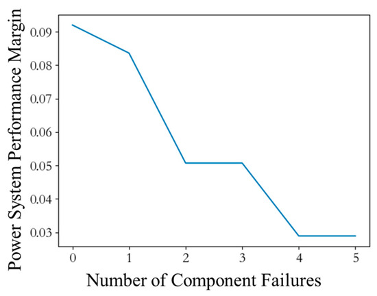
Figure 15. Variation of performance margin with the number of component failures.

5. Conclusions

This study proposes a multi-level modeling approach for Performance Margin and Belief Reliability in Redundant Systems. Unlike traditional methods, the proposed approach establishes a margin equation that explicitly considers degradation and fault states, deriving reliability based on the principle that the performance margin remains greater than zero.

• Starting from the scientific principles of Belief Reliability, the performance and margin of multi-level redundant systems are defined. A performance method, margin equation, and measurement equation that account for system faults are presented. A hierarchical BIP modeling method for complex redundant systems is proposed, defining the normal and fault states of atomic components while considering how fault behaviors influence the performance of redundant components. Consequently, the impact of redundant components on the system is reflected through variations in system performance parameters.
• To address the low computational efficiency of boundary calculations in high-dimensional topological spaces during the threshold solving process of complex redundant system performance parameters, a Boundary Search Algorithm based on pruning optimization is proposed. This method enables numerical computation of demand-threshold sets without requiring analytical expressions.
• This paper provides an efficient numerical solution approach for the threshold set of complex system requirements. Taking the multi-layer redundant power supply system of a certain industrial control equipment as an example, a performance margin model was established to identify the critical failure state, and the system belief reliability was calculated to be 0.9611, verifying the practicality of the proposed method in redundancy design and reliability evaluation.

Future research will be directed towards two primary areas. First, regarding the algorithmic complexity, while the current boundary search algorithm effectively solves the margin equations for the presented engineering case, its computational cost in extremely high-dimensional spaces remains a challenge. Future work will explore the scalability of the algorithm, investigating advanced heuristic techniques to further optimize the complexity for systems with massive module counts and higher levels of redundancy. Finally, we intend to examine the effect of interdependencies between module parameters on the overall system reliability, with particular focus on how these dependencies influence the accuracy and sensitivity of the reliability assessments under the assumptions made in this study.

References

- Benabid, R.; Merrouche, D.; Bourenane, A.; Alzbutas, R. Reliability Assessment of Redundant Electrical Power Supply Systems Using Fault Tree Analysis, Reliability Block Diagram, and Monte Carlo Simulation Methods. In Proceedings of the 2018 International Conference on Electrical Sciences and Technologies in Maghreb (CISTEM); IEEE: New York, YN, USA, 2018; pp. 1–7. [Google Scholar]
- Kaiser, B.; Gramlich, C.; Förster, M. State/Event Fault Trees—A Safety Analysis Model for Software-Controlled Systems. Reliab. Eng. Syst. Saf. 2007, 92, 1521–1537. [Google Scholar] [CrossRef]
- Ereau, J.-F.; Saleman, M.; Valette, R.; Demmou, H. Petri Nets for the Evaluation of Redundant Systems. Reliab. Eng. Syst. Saf. 1997, 55, 95–104. [Google Scholar] [CrossRef]
- Chen, Q.; Zhang, J. Evolution Model of Emergency Material Supply Chain Stress Based on Stochastic Petri Nets—A Case Study of Emergency Medical Material Supply Chains in China. Systems 2025, 13, 423. [Google Scholar] [CrossRef]
- Boudali, H.; Crouzen, P.; Stoelinga, M. A Rigorous, Compositional, and Extensible Framework for Dynamic Fault Tree Analysis. IEEE Trans. Dependable Secur. Comput. 2010, 7, 128–143. [Google Scholar] [CrossRef]
- Zhai, Q.; Peng, R.; Xing, L.; Yang, J. Binary Decision Diagram-Based Reliability Evaluation of k-out-of-(n plus k) Warm Standby Systems Subject to Fault-Level Coverage. Proc. Inst. Mech. Eng. Part O-J. Risk Reliab. 2013, 227, 540–548. [Google Scholar] [CrossRef]
- Wang, W.; Xiong, J.; Xie, M. A Study of Interval Analysis for Cold-Standby System Reliability Optimization under Parameter Uncertainty. Comput. Ind. Eng. 2016, 97, 93–100. [Google Scholar] [CrossRef]
- Ahmadi, M.; Shekhar, A.; Bauer, P. Impact of the Various Components Consideration on Choosing Optimal Redundancy Strategy in MMC. In Proceedings of the 2022 IEEE 20th International Power Electronics and Motion Control Conference (PEMC); IEEE: New York, YN, USA, 2022; pp. 21–26. [Google Scholar]
- Dugan, J.B.; Bavuso, S.J.; Boyd, M.A. Dynamic Fault-Tree Models for Fault-Tolerant Computer Systems. IEEE Trans. Reliab. 1992, 41, 363–377. [Google Scholar] [CrossRef]
- Popa, C.; Stefanov, O.; Goia, I.; Nistor, F. A Hybrid Fault Tree–Fuzzy Logic Model for Risk Analysis in Multimodal Freight Transport. Systems 2025, 13, 429. [Google Scholar] [CrossRef]
- Zhang, P.; Chan, K.W. Reliability Evaluation of Phasor Measurement Unit Using Monte Carlo Dynamic Fault Tree Method. IEEE Trans. Smart Grid 2012, 3, 1235–1243. [Google Scholar] [CrossRef]
- Zhong, C.; Jin, H. A Novel Optimal Preventive Maintenance Policy for a Cold Standby System Based on Semi-Markov Theory. Eur. J. Oper. Res. 2014, 232, 405–411. [Google Scholar] [CrossRef]
- Fathizadeh, M.; Khorshidian, K. An Alternative Approach to Reliability Analysis of Cold Standby Systems. Commun. Stat.—Theory Methods 2016, 45, 6471–6480. [Google Scholar] [CrossRef]
- Zeng, Y.; Duan, R.; Huang, S.; Feng, T. Reliability Analysis for Complex Systems Based on Generalized Stochastic Petri Nets and EDA Approach Considering Common Cause Failure. Eng. Comput. 2019, 37, 1513–1530. [Google Scholar] [CrossRef]
- Tannous, O.; Xing, L.; Dugan, J.B. Reliability Analysis of Warm Standby Systems Using Sequential BDD. In Proceedings of the Annual Reliability and Maintainability Symposium (Rams), 2011 proceedings; IEEE: New York, YN, USA, 2011. [Google Scholar]
- Jia, H.; Ding, Y.; Peng, R.; Song, Y. Reliability Evaluation for Demand-Based Warm Standby Systems Considering Degradation Process. IEEE Trans. Reliab. 2017, 66, 795–805. [Google Scholar] [CrossRef]
- Mo, Y.; Xing, L. An Enhanced Decision Diagram-Based Method for Common-Cause Failure Analysis. Proc. Inst. Mech. Eng. Part O-J. Risk Reliab. 2013, 227, 557–566. [Google Scholar] [CrossRef]
- Yeh, W.-C.; Huang, C.-L.; Wu, H.-S. An Improved d-MP Algorithm for Reliability of Logistics Delivery Considering Speed Limit of Different Roads. Signals 2022, 3, 895–910. [Google Scholar] [CrossRef]
- Levitin, G.; Xing, L.; Dai, Y. Optimizing Dynamic Performance of Multistate Systems With Heterogeneous 1-Out-of-N Warm Standby Components. IEEE Trans. Syst. Man Cybern.-Syst. 2018, 48, 920–929. [Google Scholar] [CrossRef]
- Levitin, G.; Xing, L.; Ben-Haim, H.; Huang, H.-Z. Dynamic Demand Satisfaction Probability of Consecutive Sliding Window Systems with Warm Standby Components. Reliab. Eng. Syst. Saf. 2019, 189, 397–405. [Google Scholar] [CrossRef]
- Kang, R.; Zhang, Q.; Zeng, Z.; Zio, E.; Li, X. Measuring Reliability under Epistemic Uncertainty: Review on Non-Probabilistic Reliability Metrics. Chin. J. Aeronaut. 2016, 29, 571–579. [Google Scholar] [CrossRef]
- Zeng, Z.; Wen, M.; Kang, R. Belief Reliability: A New Metrics for Products’ Reliability. Fuzzy Optim. Decis. Mak. 2013, 12, 15–27. [Google Scholar] [CrossRef]
- Wang, Y.; Kang, R.; Chen, Y. Belief Reliability Modeling for the Two-Phase Degradation System with a Change Point under Small Sample Conditions. Comput. Ind. Eng. 2022, 173, 108697. [Google Scholar] [CrossRef]
- Li, Y.; Chen, Y.; Zhang, Q.; Kang, R. Belief Reliability Analysis of Multi-State Deteriorating Systems under Epistemic Uncertainty. Inf. Sci. 2022, 604, 249–266. [Google Scholar] [CrossRef]
- Chen, Y.; Wang, Y.; Kang, R. Epistemic Uncertainty Propagation and Reliability Evaluation of Feedback Control System. IEEE Trans. Reliab. 2024, 73, 521–535. [Google Scholar] [CrossRef]
- Chen, Y.; Wang, Y.; Li, S.; Kang, R. Hybrid Uncertainty Quantification of Dependent Competing Failure Process with Chance Theory. Reliab. Eng. Syst. Saf. 2023, 230, 108958. [Google Scholar] [CrossRef]
- Basu, A.; Bozga, M.; Sifakis, J. Modeling heterogeneous real-time components in BIP. In Proceedings of the Fourth IEEE International Conference on Software Engineering and Formal Methods (SEFM 2006); IEEE: New York, YN, USA, 2006; pp. 3–12. [Google Scholar] [CrossRef]
- Basu, A.; Bensalem, S.; Bozga, M.; Bourgos, P.; Sifakis, J. Rigorous System Design: The BIP Approach; Lecture Notes in Computer Science (MEMICS 2011); Springer: Berlin/Heidelberg, Germany, 2012; Volume 7119. [Google Scholar] [CrossRef]
- Bliudze, S.; Sifakis, J. The Algebra of Connectors—Structuring Interaction in BIP. IEEE Trans. Comput. 2008, 57, 1315–1330. [Google Scholar] [CrossRef]
Disclaimer/Publisher’s Note: The statements, opinions and data contained in all publications are solely those of the individual author(s) and contributor(s) and not of MDPI and/or the editor(s). MDPI and/or the editor(s) disclaim responsibility for any injury to people or property resulting from any ideas, methods, instructions or products referred to in the content. |
© 2026 by the authors. Licensee MDPI, Basel, Switzerland. This article is an open access article distributed under the terms and conditions of the Creative Commons Attribution (CC BY) license.