Novel Conformable Fractional Order Unbiased Kernel Regularized Nonhomogeneous Grey Model and Its Applications in Energy Prediction

Abstract

Grey models have attracted considerable attention as a time series forecasting tool in recent years. Nevertheless, the linear characteristics of the differential equations on which traditional grey models rely frequently result in inadequate predictive accuracy and applicability when addressing intricate nonlinear systems. This study introduces a conformable fractional order unbiased kernel-regularized nonhomogeneous grey model (CFUKRNGM) based on statistical learning theory to address these limitations. The proposed model initially uses a conformable fractional-order accumulation operator to derive distribution information from historical data. A novel regularization problem is then formulated, thereby eliminating the bias term from the kernel-regularized nonhomogeneous grey model (KRNGM). The parameter estimation of the CFUKRNGM model requires solving a linear equation with a lower order than the KRNGM model, and is automatically calibrated through the Bayesian optimization algorithm. Experimental results show that the CFUKRNGM model achieves superior prediction accuracy and greater generalization performance compared to both the KRNGM and traditional grey models.

1. Introduction

Numerous nations worldwide are presently seeing a transformation in their energy consumption frameworks. A multitude of scholars have exerted considerable effort to devise energy forecasting methodologies intended to precisely estimate national energy use. Lu et al. conducted a literature survey on building energy prediction using artificial neural networks (ANNs), highlighting their potential to improve prediction accuracy and efficiency in energy management systems [1]. Similarly, Wang et al. studied the application of Random Forest algorithms for hourly building energy prediction, revealing their higher precision compared to standard techniques [2]. Fan et al. proposed deep learning-based feature engineering methods to enhance building energy prediction models, leveraging neural networks to automatically extract features from large-scale data, resulting in significant improvements in forecasting accuracy [3]. Additionally, Cammarano et al. introduced the Pro-Energy model, combining solar and wind energy harvesting with wireless sensor networks and offering a promising solution for energy prediction in renewable energy systems [4]. Nevertheless, the swift acceleration of economic expansion renders several statistical models inadequate for managing the significant uncertainty in energy consumption predictions. Indeed, the economic frameworks of numerous nations worldwide have experienced substantial transformations in recent years, rendering only the most current data dependable for forecasting energy consumption. Consequently, numerous researchers have adopted forecasting models adept at managing limited sample sizes [5,6,7,8].

Grey system theory, initially introduced by Deng [9] in 1982, has gained substantial popularity in forecasting and decision-making research due to its strong performance under uncertain conditions and limited data scenarios. Among various grey models, the GM(1,1) model (or GM for short) is the most basic and widely adopted, recognized for delivering reliable forecasts even with minimal data (as few as four points) [10]. Owing to their effectiveness in handling small datasets, grey prediction models have found widespread applications in diverse fields, including traffic safety analysis [11], energy production prediction [12], energy economics forecasting [13], as well as environmental studies [14,15].

Nevertheless, traditional grey models rely on integer order accumulation, which can be inadequate for systems exhibiting strong memory effects or complex dynamics. To address this limitation, fractional calculus—capable of representing long-memory processes and refined dynamical details—has been gradually introduced into grey modeling. In 2013, Wu et al. [16] pioneered the integration of fractional order accumulation (abbreviated as FOA) into fractional grey models (abbreviated as FGM), thereby facilitating effective modeling of nonlinear sequences without additional nonlinear equations. This approach subsequently demonstrated robust performance in emission forecasting [17], clean energy production [18], space-floating target trajectories [19], and building settlement monitoring [20]. Concurrently, researchers have proposed a variety of fractional grey models for different application contexts. For example, Gao et al. [21] proposed a discrete fractional grey model aimed at forecasting China’s CO₂ emissions. Ma et al. [22] employed conformable fractional derivatives and a brute-force approach for optimizing the order. Duan et al. [23] applied particle swarm optimization (abbreviated as PSO) to enhance fractional grey models for forecasting China’s crude oil consumption. Lin et al. [24] introduced fractional operators into a time-delay polynomial grey model, improving its flexibility. Wu et al. [25] adjusted the order of fractional accumulations in GMC(1,N) to forecast electric power consumption in Shandong province. These findings collectively underscore the pronounced advantages of fractional grey models in dealing with nonlinear and nonstationary sequences.

On the other hand, conventional grey models still encounter challenges when subjected to strong nonlinearities or external disturbances. In response, scholars have put forward the nonhomogeneous grey model (abbreviated as NGM) and its various extensions [26,27,28], incorporating time-dependent or other prior information into the whitening equation to capture more complex external drivers. However, adding linear terms alone may not thoroughly capture higher-order nonlinear structures in the data. To address this shortcoming, Ma et al. [29] introduced a kernel-based regularization scheme for nonhomogeneous grey models (abbreviated as KRNGM), which maps the linear model into a high-dimensional feature space, thereby flexibly representing nonlinear dynamics. This concept is grounded in Vapnik’s work on support vector machines (abbreviated as SVMs) [30], which has already gained widespread traction in machine learning [31], clustering [32], and principal component analysis [33]. Furthermore, the least squares support vector machine (abbreviated as LS-SVM) proposed by Suykens et al. [34] has simplified kernel-based methods, enabling successful applications in image classification [35], hydropower consumption forecasting [36], and natural disaster prediction [37].

Despite these developments, existing kernel-based regularized nonhomogeneous grey models still treat the bias term as a separately estimated parameter. This approach can not only complicate the model structure but also introduce biases in parameter estimation, thereby reducing its generalization capability. In order to enhance its practical utility, this study draws on the unbiased perspective proposed by Wang et al. [38] for LS-SVM, which jointly regularizes the bias term and kernel mapping parameters to effectively suppress uncertainties arising from the bias. This unbiased strategy has been extended to multiple applications in computer vision and machine learning. For instance, Jeon et al. [39] employed unbiased learning methods to mitigate convolutional neural networks’ (abbreviated as CNN) reliance on biased training data, while de Mello et al. [40] presented an innovative active learning strategy to curtail the detrimental effects of biased sampling on model performance.

This research advances current understanding by integrating conformable fractional order accumulation into the kernel-based regularized nonhomogeneous grey model. The outcome is the conformable fractional unbiased kernel-regularized nonhomogeneous grey model (CFUKRNGM). This methodology seeks to enhance predictive precision for intricate systems through the utilization of a tunable-order accumulation operator. This operator enables the modulation of historical data weighting. Furthermore, impartial regularization is employed to alleviate overfitting induced by the bias factor. Oil production projections serve as a case study for evaluating the model’s efficacy, illustrating its practical applicability.

2. Kernel-Regularized Nonhomogeneous Grey Model

2.1. Mathematical Basis of GM(1,1)

Grey system theory asserts that real observational data frequently encompass noise, random variations, and other uncertainties, complicating the direct formulation of a dynamic equation from the raw dataset. To resolve this, grey models utilize the accumulation generation operation (AGO), which converts the differential properties of the discrete series into a more uniform sequence, thus reducing significant oscillations that may exist in the raw data. Let the original sequence be specified as

$$X^{\left(0\right)}=\left\{x^{\left(0\right)}\left(1\right),x^{\left(0\right)}\left(2\right),\dots ,x^{\left(0\right)}\left(n\right)\right\},$$

(1)

and define its first-order accumulated operation (abbreviated as 1-AGO) sequence as

$$X^{\left(1\right)}=\left\{x^{\left(1\right)}\left(1\right),x^{\left(1\right)}\left(2\right),\dots ,x^{\left(1\right)}\left(n\right)\right\},$$

(2)

where

$$x^{\left(1\right)}\left(k\right)=\sum _{i=1}^k{x}^{\left(0\right)}\left(i\right),k=1,2,\dots ,n.$$

(3)

Through the 1-AGO operation, the original series is smoothed to some extent, providing a more stable data foundation for subsequent differential equation fitting.

Once the relatively smooth sequence $X^{\left(1\right)}$ is obtained, the core assumption in grey models is that this accumulated sequence can be described by a first-order linear differential equation, namely,

$${\displaystyle \frac{d{x}^{\left(1\right)}\left(t\right)}{dt}}+a{x}^{\left(1\right)}\left(t\right)=b,$$

(4)

where a and b are constants to be estimated. This equation is referred to as the white equation of GM(1,1), which effectively maps a discrete, noise-perturbed sequence onto a relatively simple continuous dynamic system.

To relate Equation (4) to discrete observations, grey modeling introduces the concept of background values by setting

$$z^{\left(1\right)}\left(k\right)={\displaystyle \frac{1}{2}}\left[x^{\left(1\right)}\left(k\right)+x^{\left(1\right)}(k-1)\right],k=2,3,\dots ,n.$$

(5)

Here, $z^{\left(1\right)}\left(k\right)$ approximately represents the average level of $x^{\left(1\right)}\left(t\right)$ over the interval $[k-1,k]$. Meanwhile, at discrete time $t=k$, the differential equation is approximately satisfied by

$${\int }_{k-1}^{k}d{x}^{\left(1\right)}\left(t\right)=x^{\left(1\right)}\left(k\right)-x^{\left(1\right)}(k-1)=x^{\left(0\right)}\left(k\right),$$

(6)

which allows Equation (4) to be discretized at k as

$$x^{\left(0\right)}\left(k\right)+a{z}^{\left(1\right)}\left(k\right)=b,k=2,3,\dots ,n.$$

(7)

This constitutes the GM(1,1) model in discrete form. Rearranging Equation (7) yields the matrix equation

$$\mathbf{Y}=\mathbf{B}\mathbf{H},$$

(8)

where

$$\mathbf{Y}=\left(\begin{array}{c}{x}^{\left(0\right)}\left(2\right)\\ x^{\left(0\right)}\left(3\right)\\ ⋮\\ x^{\left(0\right)}\left(n\right)\end{array}\right),\mathbf{B}=\left(\begin{array}{cc}-z^{\left(1\right)}\left(2\right)& 1\\ -z^{\left(1\right)}\left(3\right)& 1\\ ⋮& ⋮\\ -z^{\left(1\right)}\left(n\right)& 1\end{array}\right),\mathbf{H}=\left(\begin{array}{c}a\\ b\end{array}\right).$$

(9)

By applying the least squares method, one obtains

$$\mathbf{H}={\left({\mathbf{B}}^{\mathrm{T}}\mathbf{B}\right)}^{-1}{\mathbf{B}}^{\mathrm{T}}\mathbf{Y},$$

(10)

thus determining the estimates of a and b. Consequently, the white equation of GM(1,1) captures, to a certain extent, the continuous evolution pattern of the sequence $X^{\left(1\right)}$.

Once a and b are determined, one can analytically solve the continuous form of Equation (4):

$${\widehat{x}}^{\left(1\right)}\left(t\right)=\left[x^{\left(0\right)}\left(1\right)-{\displaystyle \frac{b}{a}}\right]e^{-a(t-1)}+{\displaystyle \frac{b}{a}}.$$

(11)

For discrete time k, substituting $t=k$ and using $x^{\left(1\right)}\left(1\right)=x^{\left(0\right)}\left(1\right)$ yields

$${\widehat{x}}^{\left(1\right)}\left(k\right)=\left[x^{\left(0\right)}\left(1\right)-{\displaystyle \frac{b}{a}}\right]e^{-a(k-1)}+{\displaystyle \frac{b}{a}}.$$

(12)

However, GM(1,1) makes forecasts for the accumulated sequence $X^{\left(1\right)}$. To revert to the original scale $X^{\left(0\right)}$, one must perform an inverse accumulation operation (abbreviated as IAGO):

$${\widehat{x}}^{\left(0\right)}\left(k\right)={\widehat{x}}^{\left(1\right)}\left(k\right)-{\widehat{x}}^{\left(1\right)}(k-1)$$

(13)

This step yields the forecasted value of ${\widehat{x}}^{\left(0\right)}\left(k\right)$ at time k, thereby completing the overall prediction procedure.

In GM(1,1), only the linear term $a{x}^{\left(1\right)}\left(t\right)$ and a constant term b are considered. To accommodate strong nonlinearities or external disturbances, an additional nonhomogeneous term $f\left(t\right)$ is typically introduced, thus giving the whitening equation

$${\displaystyle \frac{d{x}^{\left(1\right)}\left(t\right)}{dt}}+a{x}^{\left(1\right)}\left(t\right)=f\left(t\right)+c,$$

(14)

which corresponds to the NGM(1,1,k,c) model. It allows the incorporation of more external drivers or nonlinear information under the grey model framework, thereby enhancing the depiction of complex systems. Similar to GM(1,1), discretizing $x^{\left(1\right)}\left(t\right)$ and using background values and least squares (or regularization) enables the estimation of a, c, and the parameters of $f\left(t\right)$. When $f\left(t\right)$ is unknown and strongly nonlinear, kernel methods (discussed in the following subsection) can be applied to approximate it.

2.2. Kernel-Regularized Nonhomogeneous Grey Model

As previously mentioned, the NGM(1,1,k,c) model maintains a fundamentally linear structure. To incorporate nonlinear modeling capability, this section proposes introducing kernel regularization into the nonhomogeneous grey model framework.

$${\displaystyle \frac{d{x}^{\left(1\right)}\left(t\right)}{dt}}+a{x}^{\left(1\right)}\left(t\right)=f\left(t\right)+c,$$

(15)

where $f\left(t\right)$ represents a nonlinear transformation with respect to t. If $f\left(t\right)$ is set as the identity function ($f\left(t\right)=t$), the model reduces to the NGM(1,1,k,c) form.

The whitening equation of KRNGM is

$${\displaystyle \frac{d{x}^{\left(1\right)}\left(t\right)}{dt}}+a{x}^{\left(1\right)}\left(t\right)={\mathit{w}}^T\mathit{\phi }\left(t\right)+c,$$

(16)

Here, $\mathbf{\phi }\left(t\right)$ represents a nonlinear transformation mapping inputs into a higher-dimensional feature space, while $\mathit{w}$ denotes the corresponding coefficient vector. After discretizing across the interval $[k-1,k]$ using the trapezoidal rule, the equation becomes:

$$x^{\left(0\right)}\left(k\right)+a{z}^{\left(1\right)}\left(k\right)={\mathit{w}}^T\mathit{\varphi }\left(k\right)+c,$$

(17)

where

$$z^{\left(1\right)}\left(k\right)={\displaystyle \frac{1}{2}}\left[x^{\left(1\right)}\left(k\right)+x^{\left(1\right)}(k-1)\right]\mathrm{and}\mathit{\varphi }\left(k\right)={\displaystyle \frac{1}{2}}\left[\mathit{\phi }\left(k\right)+\mathit{\phi }(k-1)\right].$$

(18)

To estimate the parameters of the KRNGM, the following optimization objective is defined:

$$\begin{array}{cc}\hfill & \underset{a,w,c}{min}\left({\displaystyle \frac{a^2}{2}}+{\displaystyle \frac{{\mathit{w}}^T\mathit{w}}{2}}+{\displaystyle \frac{\gamma }{2}}\sum _{j=2}^n{e}_j^2\right),\hfill \\ \hfill & \mathrm{s}.\mathrm{t}.e_j=x^{\left(0\right)}\left(j\right)+a{z}^{\left(1\right)}\left(j\right)-{\mathit{w}}^T\mathbf{\varphi }\left(j\right)-c,j=2,\dots ,n,\hfill \end{array}$$

(19)

where $\gamma$ is a regularization coefficient that balances the model’s smoothness and fitting error. To solve this quadratic program with linear constraints, the Lagrangian is formulated as

$$L={\displaystyle \frac{a^2}{2}}+{\displaystyle \frac{{\mathit{w}}^T\mathit{w}}{2}}+{\displaystyle \frac{\gamma }{2}}\sum _{j=2}^n{e}_j^2+\sum _{j=2}^n{\lambda }_j\left[x^{\left(0\right)}\left(j\right)+a{z}^{\left(1\right)}\left(j\right)-{\mathit{w}}^T\mathit{\varphi }\left(j\right)-c-e_j\right].$$

(20)

According to the KKT conditions, one obtains

$$\left\{\begin{array}{cc}\hfill {\displaystyle \frac{\partial L}{\partial a}}=0& \Rightarrow a=\sum _{j=2}^n{\lambda }_j{z}^{\left(1\right)}\left(j\right),\hfill \\ \hfill {\displaystyle \frac{\partial L}{\partial \mathit{w}}}=0& \Rightarrow \mathit{w}=\sum _{j=2}^n{\lambda }_j\mathit{\varphi }\left(j\right),\hfill \\ \hfill {\displaystyle \frac{\partial L}{\partial c}}=0& \Rightarrow \sum _{j=2}^n{\lambda }_j=0,\hfill \\ \hfill {\displaystyle \frac{\partial L}{\partial e_j}}=0& \Rightarrow e_j={\displaystyle \frac{{\lambda }_j}{\gamma }},\hfill \\ \hfill {\displaystyle \frac{\partial L}{\partial {\lambda }_j}}=0& \Rightarrow x^{\left(0\right)}\left(j\right)+a{z}^{\left(1\right)}\left(j\right)-{\mathit{w}}^T\mathit{\varphi }\left(j\right)-c=e_j.\hfill \end{array}\right.$$

(21)

By eliminating a, w, and $e_j$ from the KKT conditions, one obtains the following linear system:

$$\left[\begin{array}{cc}0& {\mathbf{1}}_{n-1}^{\top }\\ {\mathbf{1}}_{n-1}& \Omega +{\gamma }^{-1}{I}_{n-1}\end{array}\right]\left[\begin{array}{c}c\\ \mathbf{\lambda }\end{array}\right]=\left[\begin{array}{c}0\\ \mathit{Y}\end{array}\right],$$

(22)

where

$$\begin{array}{cc}\hfill {\mathbf{1}}_{n-1}& ={[1,1,\dots ,1]}_{n-1}^{\top },\hfill \\ \hfill \Omega & ={\left({\mathit{\varphi }}^T\left(i\right)\mathit{\varphi }\left(j\right)-z^{\left(1\right)}\left(i\right)z^{\left(1\right)}\left(j\right)\right)}_{(n-1)\times (n-1)},\hfill \\ \hfill \mathbf{\lambda }& ={[{\lambda }_2,{\lambda }_3,\dots ,{\lambda }_n]}^{\top },\hfill \\ \hfill \mathit{Y}& ={[x^{\left(0\right)}\left(2\right),x^{\left(0\right)}\left(3\right),\dots ,x^{\left(0\right)}\left(n\right)]}^{\top }.\hfill \end{array}$$

and ${\mathit{I}}_{n-1}$ is the $(n-1)$-dimensional identity matrix whose diagonal elements are 1 and whose off-diagonal entries are 0.

By solving the above system, one obtains ${\lambda }_j$ and c. Using the first relation in the KKT conditions provides the parameter a. If the kernel function $K(·,·)$ satisfies $\mathit{\phi }\left(i\right)·\mathit{\phi }\left(j\right)=K(i,j)$, explicit construction of $\mathit{\phi }$ vectors can be avoided. Through this regularization process, one thereby determines the main parameters of the KRNGM model.

2.3. Time-Response Series of the KRNGM

Once the parameters of the KRNGM are determined, the forecasted sequences ${\widehat{X}}^{\left(1\right)}$ and ${\widehat{X}}^{\left(0\right)}$ can be calculated. The initial condition is set as ${\widehat{x}}^{\left(1\right)}\left(1\right)=x^{\left(1\right)}\left(1\right)=x^{\left(0\right)}\left(1\right)$, then

$${\widehat{x}}^{\left(1\right)}\left(t\right)=x^{\left(0\right)}\left(1\right)e^{-a(t-1)}+{\int }_1^t{e}^{-a(t-\tau )}\Psi \left(\tau \right)d\tau ,$$

(23)

where $\Psi \left(t\right)={\mathit{w}}^T\mathit{\phi }\left(t\right)+c$. According to $\mathit{w}={\sum }_{j=2}^n{\lambda }_j\mathit{\varphi }\left(j\right)$, one obtains

$${\mathit{w}}^T\mathit{\phi }\left(t\right)={\displaystyle \frac{1}{2}}\sum _{j=2}^n{\lambda }_j\left[\mathit{\phi }\left(j\right)+\mathit{\phi }(j-1)\right]·\mathit{\phi }\left(t\right)={\displaystyle \frac{1}{2}}\sum _{j=2}^n{\lambda }_j\left[K_{j,t}+K_{j-1,t}\right].$$

(24)

Applying the trapezoidal rule to the integral term in Equation (23) yields

$${\widehat{x}}^{\left(1\right)}\left(k\right)=x^{\left(0\right)}\left(1\right)e^{-a(k-1)}+{\displaystyle \frac{1}{2}}\sum _{\tau =2}^k\left[e^{-a(k-\tau )}\Psi \left(\tau \right)+e^{-a(k-\tau +1)}\Psi (\tau -1)\right].$$

(25)

Finally, to obtain the predicted original series ${\widehat{X}}^{\left(0\right)}$, one applies the difference:

$${\widehat{x}}^{\left(0\right)}\left(k\right)={\widehat{x}}^{\left(1\right)}\left(k\right)-{\widehat{x}}^{\left(1\right)}(k-1).$$

(26)

Through these steps, the KRNGM completes its overall prediction process.

3. Proposed Conformable Fractional Unbiased Kernel Regularized Nonhomogeneous Grey Model

This section introduces an unbiased kernel-regularized nonhomogeneous grey model with conformable fractional order (CFUKRNGM). The CFUKRNGM combines the advantages of the conformable fractional grey model (CFGM) and kernel-regularized models (KRNGM), utilizing an unbiased parameter estimation approach. The suggested CFUKRNGM improves conventional grey models in the analysis of intricate dynamic systems. It achieves this by integrating the flexible memory attributes of conformable fractional-order accumulation. Furthermore, it utilizes the nonlinear modeling potential afforded by kernel regularization.

3.1. The Definition of Conformable Fractional Accumulation and Difference

This subsection presents the definitions of conformable fractional accumulation and difference.

Definition 1.

Given a differential function f, the α order conformable fractional accumulation (abbreviated as α-CFA) [28] of f with α order is

$${\nabla }^{\alpha }f\left(k\right)=\sum _{i=1}^k\left({\displaystyle \genfrac{}{}{0pt}{}{k-i+\left[\alpha \right]-1}{k-i}}\right){\displaystyle \frac{f\left(i\right)}{i^{\left[\alpha \right]-\alpha }}},\alpha >0,$$

(27)

where $\left({\displaystyle \genfrac{}{}{0pt}{}{k-i+\left[\alpha \right]-1}{k-i}}\right)={\displaystyle \frac{(k-i+[\alpha ]-1)!}{(k-i)!\left(\right[\alpha ]-1)!}}$, and $\left[.\right]$ denotes the ceil function, which represents the smallest integer no larger than α.

Definition 2.

Given a differential function f, the α order conformable fractional difference (abbreviated as α-CFD) [28] of f with α order is

$${\Delta }^{\alpha }f\left(k\right)=k^{\left[\alpha \right]-\alpha }\sum _{i=1}^k{(-1)}^{k-i}\left({\displaystyle \genfrac{}{}{0pt}{}{\left[\alpha \right]}{k-i}}\right)f\left(i\right),\alpha >0,$$

(28)

where $\left({\displaystyle \genfrac{}{}{0pt}{}{\left[\alpha \right]}{k-i}}\right)={\displaystyle \frac{\left[\alpha \right]!}{\left(\right[\alpha ]-k+i)!(k-i)!}}$.

The conformable fractional accumulation and the conformable fractional difference satisfy the following relationship:

$${\Delta }^{\alpha }{\nabla }^{\alpha }f\left(k\right)=f\left(k\right),\alpha >0.$$

(29)

Definition 1 is utilized to calculate the cumulative value of the original sequence, whereas Definition 2 determines the recovery value of the model’s fitted sequence. It is significant because, in comparison to conventional fractional order accumulation (FOA), both conformable fractional order accumulation and difference are more straightforward to execute.

3.2. The Conformable Fractional Unbiased Kernel Regularized Nonhomogeneous Grey Model

Based on the definitions of $\alpha$-CFA and $\alpha$-CFD, the CFUKRNGM model is formulated, and the corresponding implementation steps are described as follows.

For the given initial sequence $X^{\left(0\right)}=\left(x^{\left(0\right)}\left(1\right),x^{\left(0\right)}\left(2\right),\dots ,x^{\left(0\right)}\left(n\right)\right)$, we first define its $\alpha$-CFA sequence as $X^{\left(\alpha \right)}=\left(x^{\left(\alpha \right)}\left(1\right),x^{\left(\alpha \right)}\left(2\right),\dots ,x^{\left(\alpha \right)}\left(n\right)\right)$, with the following relationship:

$$x^{\left(\alpha \right)}\left(k\right)={\nabla }^{\alpha }{x}^{\left(0\right)}\left(k\right)=\left\{\begin{array}{cc}\sum _{j=1}^k{\displaystyle \frac{x^{\left(0\right)}\left(j\right)}{j^{\left[\alpha \right]-\alpha }}},\hfill & \hfill 0<\alpha \le 1,\\ \sum _{j=1}^k{x}^{(\alpha -1)}\left(j\right),\hfill & \hfill \alpha >1.\end{array}\right.$$

(30)

Similar to the KRNGM model, the CFUKRNGM is expressed as

$${\displaystyle \frac{d{x}^{\left(\alpha \right)}\left(t\right)}{dt}}+a{x}^{\left(\alpha \right)}\left(t\right)={\mathit{w}}^T\mathit{\phi }\left(t\right)+c.$$

(31)

The differential Equation (31) is referred to as the whitening equation of the CFUKRNGM model. When $\alpha =1$, it reduces to the KRNGM model proposed by Ma et al. [22]. Specifically, if $\mathit{\phi }$ is defined as an identity map and $\alpha =1$, the CFUKRNGM model (31) simplifies to the NGM(1, 1, k, c) model.

3.3. Parameter Estimation for the CFUKRNGM Model

To determine the parameters of the KRNGM model, we begin by discretizing the differential Equation (31). By integrating (31) over the interval $[k-1,k]$, the resulting expression is obtained as follows:

$${\int }_{k-1}^{k}d{x}^{\left(\alpha \right)}\left(t\right)+a{\int }_{k-1}^k{x}^{\left(\alpha \right)}\left(t\right)dt={\mathit{w}}^T{\int }_{k-1}^k\mathit{\phi }\left(t\right)dt+{\int }_{k-1}^{k}cdt.$$

(32)

Noting that ${\int }_{k-1}^{k}d{x}^{\left(\alpha \right)}\left(t\right)=x^{\left(\alpha \right)}\left(k\right)-x^{\left(\alpha \right)}(k-1)$, and ${\int }_{k-1}^{k}cdt=c$. To discretize the remaining integral terms involving $x^{\left(\alpha \right)}\left(t\right)$ and $\mathit{\phi }\left(t\right)$, we apply the two-point trapezoidal rule, which approximates the integral over $[k-1,k]$ as the average of the values at the endpoints of the interval.

$$x^{\left(\alpha \right)}\left(k\right)-x^{\left(\alpha \right)}(k-1)+a{z}^{\left(\alpha \right)}\left(k\right)={\mathit{w}}^T\mathit{\varphi }\left(k\right)+c,$$

(33)

where

$$z^{\left(\alpha \right)}\left(k\right)={\displaystyle \frac{1}{2}}\left(x^{\left(\alpha \right)}\left(k\right)+x^{\left(\alpha \right)}(k-1)\right)$$

(34)

and

$$\mathit{\varphi }\left(k\right)={\displaystyle \frac{1}{2}}\left(\mathit{\phi }\left(k\right)+\mathit{\phi }(k-1)\right).$$

(35)

The exact form of the nonlinear mapping $\mathit{\phi }$ being unknown necessitates a regularization method. The structural risk reduction technique in the KRNGM model notably omits the bias factor c, potentially leading to overfitting and diminishing the model’s generalization capability. This paper integrates the bias term c into the structural risk reduction framework, creating an innovative regularized optimization problem for parameter estimation of the CFUKRNGM model. The mathematical formulation of this optimization problem is expressed as follows:

$$\begin{array}{cc}\hfill & min{\displaystyle \frac{a^2}{2}}+{\displaystyle \frac{1}{2}}{\mathit{w}}^T\mathit{w}+{\displaystyle \frac{c^2}{2{\theta }^2}}+{\displaystyle \frac{\gamma }{2}}\sum e_j^2,\hfill \\ \hfill & \mathrm{s}.\mathrm{t}.e_j=x^{\left(\alpha \right)}\left(j\right)-x^{\left(\alpha \right)}(j-1)+a{z}^{\left(\alpha \right)}\left(j\right)-{\mathit{w}}^T\mathit{\varphi }\left(j\right)-c\hfill \end{array}$$

(36)

Let ${\mathit{w}}_1={\left[{\mathit{w}}^T,{\displaystyle \frac{c}{\theta }}\right]}^T$ and ${\left[{\mathit{\varphi }}^T\left(j\right),\theta \right]}^T={\mathit{\varphi }}_1\left(j\right)$, then the optimization problem (36) can be rewritten as

$$\begin{array}{cc}\hfill & min{\displaystyle \frac{a^2}{2}}+{\displaystyle \frac{1}{2}}{\mathit{w}}_1^T{\mathit{w}}_1+{\displaystyle \frac{\gamma }{2}}\sum e_j^2,\hfill \\ \hfill & \mathrm{s}.\mathrm{t}.e_j=x^{\left(\alpha \right)}\left(j\right)-x^{\left(\alpha \right)}(j-1)+a{z}^{\left(\alpha \right)}\left(j\right)-{\mathit{w}}_1^T{\mathit{\varphi }}_1\left(j\right)\hfill \end{array}$$

(37)

where $\theta$ is a hyperparameter of the CFUKRNGM model. Notice that at this stage, ${\mathit{w}}^T\mathit{\phi }\left(t\right)+c={\mathit{w}}_1^T{\mathit{\phi }}_1\left(t\right)$, where ${\left[{\mathit{\phi }}^T\left(j\right),\theta \right]}^T={\mathit{\phi }}_1\left(j\right)$. Clearly,

$${\mathit{\varphi }}_1\left(k\right)={\displaystyle \frac{1}{2}}\left({\mathit{\phi }}_1\left(k\right)+{\mathit{\phi }}_1(k-1)\right)={\left[{\displaystyle \frac{1}{2}}\left({\mathit{\phi }}^T\left(k\right)+{\mathit{\phi }}^T(k-1)\right),\theta \right]}^T.$$

(38)

The problem (37) is essentially a quadratic programming problem with linear constraints, and therefore, we only need to find its extremum point. We first define the Lagrangian function as

$$L={\displaystyle \frac{a^2}{2}}+{\displaystyle \frac{1}{2}}{\mathit{w}}_1^T{\mathit{w}}_1+{\displaystyle \frac{\gamma }{2}}\sum e_j^2+\sum {\lambda }_j\left[x^{\left(\alpha \right)}\left(j\right)-x^{\left(\alpha \right)}(j-1)+a{z}^{\left(\alpha \right)}\left(j\right)-{\mathit{w}}_1^T{\mathit{\varphi }}_1\left(j\right)-e_j\right].$$

(39)

The Karush–Kuhn–Tucker (abbreviated as KKT) conditions for problem (39) are given by the following:

$$\left\{\begin{array}{cc}\hfill {\displaystyle \frac{\partial L}{\partial a}}& =a+\sum _{j=2}^n{\lambda }_j{z}^{\left(\alpha \right)}\left(j\right)=0\Rightarrow a=-\sum _{j=2}^n{\lambda }_j{z}^{\left(\alpha \right)}\left(j\right),\hfill \\ \hfill {\displaystyle \frac{\partial L}{\partial {\mathit{w}}_1}}& ={\mathit{w}}_1-\sum _{j=2}^n{\lambda }_j\left[{\mathit{\varphi }}_1\left(j\right)\right]=0\Rightarrow {\mathit{w}}_1=\sum _{j=2}^n{\lambda }_j{\left[{\mathit{\varphi }}^T\left(j\right),\theta \right]}^T,\hfill \\ \hfill {\displaystyle \frac{\partial L}{\partial e_j}}& =\gamma e_j-{\lambda }_j=0\Rightarrow e_j={\displaystyle \frac{{\lambda }_j}{\gamma }},\hfill \\ \hfill {\displaystyle \frac{\partial L}{\partial {\lambda }_j}}& =0\Rightarrow x^{\left(\alpha \right)}\left(j\right)-x^{\left(\alpha \right)}(j-1)+a{z}^{\left(\alpha \right)}\left(j\right)-{\mathit{w}}_1^T{\mathit{\varphi }}_1\left(j\right)=e_j.\hfill \end{array}\right.$$

(40)

Set $x^{\left(\alpha \right)}\left(j\right)-x^{\left(\alpha \right)}(j-1)=y^{\left(\alpha \right)}\left(j\right)$. By eliminating a, ${\mathit{w}}_1$, and $e_j$, we obtain

$$y^{\left(\alpha \right)}\left(j\right)=\sum _{i=2}^n{\lambda }_i{z}^{\left(\alpha \right)}\left(j\right)z^{\left(\alpha \right)}\left(i\right)+\sum _{i=2}^n{\lambda }_i\left[{\mathit{\varphi }}^T\left(i\right),\theta \right]\left[\begin{array}{c}\mathit{\varphi }\left(j\right)\\ \theta \end{array}\right]+e_j,j=2,3,\dots ,n.$$

(41)

The KKT conditions are equivalent to the following set of linear equations:

$$({\gamma }^{-1}\mathit{I}+\Omega )\mathbf{\lambda }=\mathit{y},$$

(42)

where

$$\begin{array}{cc}\hfill {\mathit{y}}_k& =x^{\left(\alpha \right)}\left(k\right)-x^{\left(\alpha \right)}(k-1),\hfill \\ \hfill \mathbf{\lambda }& ={({\lambda }_2,\dots ,{\lambda }_n)}^T,\hfill \\ \hfill {\Omega }_{ij}& =z^{\left(\alpha \right)}\left(i\right)z^{\left(\alpha \right)}\left(j\right)+{\mathit{\varphi }}_1^T\left(i\right){\mathit{\varphi }}_1\left(j\right),\hfill \end{array}$$

(43)

and $\mathit{I}$ represents an identity matrix of dimension $(n-1)$ with ones on the diagonal and zeros elsewhere. The parameter a is derived from the initial equation within these conditions (40).

Using the definition of ${\mathit{\varphi }}_1$ in (38), we have

$$\begin{array}{cc}\hfill {\mathit{\varphi }}_1\left(i\right)·{\mathit{\varphi }}_1\left(j\right)& ={\displaystyle \frac{1}{4}}\left(\phi \left(i\right)+\phi (i-1)\right)·\left(\phi \left(j\right)+\phi (j-1)\right)+{\theta }^2\hfill \\ \hfill & ={\displaystyle \frac{1}{4}}\left(\phi \left(i\right)·\phi \left(j\right)+\phi (i-1)·\phi \left(j\right)+\phi \left(i\right)·\phi (j-1)+\phi (i-1)·\phi (j-1)\right)+{\theta }^2\hfill \\ \hfill & ={\displaystyle \frac{1}{4}}\left(K_{ij}+K_{i-1,j}+K_{i,j-1}+K_{i-1,j-1}\right)+{\theta }^2\hfill \end{array}$$

(44)

3.4. The Time Response Series of the CFUKRNGM

The differential equation, under the initial condition ${\widehat{x}}^{\left(1\right)}\left(1\right)=x^{\left(1\right)}\left(1\right)=x^{\left(0\right)}\left(1\right)$, can be solved by applying the method of variation of parameters from differential equations, leading to the following solution:

$${\widehat{x}}^{\left(1\right)}\left(t\right)=x^{\left(0\right)}\left(1\right)e^{-a(t-1)}+{\int }_1^t{e}^{-a(t-\tau )}{\Psi }_1\left(\tau \right)d\tau .$$

(45)

where

$${\Psi }_1\left(\tau \right)d\tau ={\mathit{w}}_1^T{\mathit{\phi }}_1\left(t\right).$$

(46)

From the second equation in the KKT conditions (40), expressed as ${\mathit{w}}_1={\sum }_{j=2}^n{\lambda }_j\mathit{\varphi }\left(j\right)$, the nonlinear function ${\mathit{w}}_1^T{\mathit{\phi }}_1\left(t\right)$ can be reformulated as

$${\mathit{w}}_1^T{\mathit{\phi }}_1\left(t\right)=\left[\sum _{j=2}^n{\lambda }_j{\varphi }_1\left(j\right)\right]·{\phi }_1\left(t\right)={\displaystyle \frac{1}{2}}\sum _{j=2}^n{\lambda }_j\left[{\mathit{\phi }}^T\left(j\right)+{\mathit{\phi }}^T(j-1),2\theta \right]\left[\begin{array}{c}\mathit{\phi }\left(j\right)\\ \theta \end{array}\right].$$

(47)

By substituting (44) into (47), we obtain

$${\mathit{w}}^T\mathbf{\phi }\left(t\right)={\displaystyle \frac{1}{2}}\sum _{j=2}^n{\lambda }_j[\phi \left(j\right)+\phi (j-1)]·\phi \left(t\right)={\displaystyle \frac{1}{2}}\sum _{j=2}^n{\lambda }_j\left[K_{j,t}+K_{j-1,t}+2{\theta }^2\right]$$

(48)

To discretize the integral in (45), we apply the two-point trapezoidal rule, resulting in the discrete-time equivalent:

$${\widehat{x}}^{\left(1\right)}\left(k\right)=x^{\left(0\right)}\left(1\right)e^{-a(k-1)}+{\displaystyle \frac{1}{2}}\sum _{\tau =2}^k\left[e^{-a(k-\tau )}{\Psi }_1\left(\tau \right)+e^{-a(k-\tau +1)}{\Psi }_1(\tau -1)\right].$$

(49)

Finally, the predicted values for $x^{\left(0\right)}$ are obtained as

$${\widehat{x}}^{\left(0\right)}\left(k\right)={\Delta }^{\alpha }{\widehat{x}}^{\left(\alpha \right)}\left(k\right)=k^{\left[\alpha \right]-\alpha }{\Delta }^n{\widehat{x}}^{\left(\alpha \right)}\left(k\right),\alpha \in (n,n+1].$$

(50)

4. Parameters Optimization of CFUKRNGM Model

This section focuses on the optimization of the hyperparameters for the CFUKRNGM model. The performance of the model is highly dependent on the selection of these hyperparameters, which control the trade-off between model complexity and fitting accuracy. To identify the optimal set of parameters, we employ the Bayesian optimization algorithm, an efficient global optimization algorithm that can effectively adjust hyperparameters in high-dimensional spaces.

4.1. Optimization Strategies for Hyperparameters

It is worth noting that, given the known kernel function parameter $\sigma$, regularization coefficient $\gamma$, unbiased coefficient $\theta$, and accumulation order $\alpha$, the system parameters in the new model can be estimated. We select the parameters that minimize the mean absolute percentage error as the optimal parameters, with the mathematical expression given by

$$\begin{array}{cc}\hfill \underset{\Theta }{min}& \mathrm{MAPE}={\displaystyle \frac{1}{n}}\sum _{i=1}^n\left|{\displaystyle \frac{{\widehat{x}}^{\left(0\right)}\left(i\right)-x^{\left(0\right)}\left(i\right)}{x^{\left(0\right)}\left(i\right)}}\right|\times 100\%\hfill \end{array}$$

(51)

where $\Theta$ represents the hyperparameter vector of each model.If the parameter optimization objective is the CFUKRNGM model, then $\Theta =\left(\sigma ,\gamma ,\lambda ,\alpha \right)$. If the parameter optimization objective is the KRNGM model, then $\Theta =\left(\sigma ,\gamma \right)$.

4.2. Bayesian Optimization Algorithm

As indicated by Equation (51), this function exhibits nonlinear properties, making it challenging to derive an analytical solution using conventional methods. In the field of parameter optimization, numerous strategies have been proposed by researchers to enhance model performance and accuracy. Traditional optimization methods, such as grid search [41] and random search [42], are widely applied in hyperparameter tuning. In addition, another class of optimization methods involves heuristic algorithms, such as genetic algorithms [43], PSO [44], and simulated annealing [45]. These methods do not rely on gradient information but instead simulate random behaviors observed in nature or physical processes to find the optimal solution. While these approaches can effectively handle complex optimization problems, they may suffer from early convergence and require longer computational times. With the rapid development of machine learning, the Bayesian optimization algorithm [46] has emerged as a global optimization method based on probabilistic models.

Bayesian optimization is a global optimization technique based on probability theory. It is especially efficacious for optimizing black-box functions. The fundamental concept is to develop a surrogate model that estimates the actual objective function. Gaussian processes are frequently employed for surrogate modeling. The optimization process is directed by an acquisition function that facilitates the efficient identification of the global optimum. Consider the input dataset $X=\{{\mathit{x}}_1,{\mathit{x}}_2,\dots ,{\mathit{x}}_n\}$ and corresponding observed outputs $\mathbf{y}=\{y_1,y_2,\dots ,y_n\}$, where each observed value $y_i=f\left({\mathit{x}}_i\right)+{ϵ}_i$ includes a noise term ${ϵ}_i$, which is independently and identically distributed.

Assumes that the objective function $f\left(\mathit{x}\right)$ is drawn from a gaussian process distribution:

$$f\left(\mathit{x}\right)\sim \mathcal{GP}(m\left(\mathit{x}\right),k(\mathit{x},{\mathit{x}}^{\prime }))$$

(52)

where $m\left(\mathit{x}\right)$ is the mean function, typically taken as $m\left(\mathit{x}\right)=0$, and $k(\mathit{x},{\mathit{x}}^{\prime })$ is the covariance function or kernel, which defines the correlation between different input points.

Based on the Gaussian process model, the predicted value of the objective function at a new input point ${\mathit{x}}^{*}$ can be obtained. Considering the existing observed data points $\mathit{X}$ and their corresponding outputs $\mathit{y}$, the joint distribution between the observed outputs and the prediction at ${\mathit{x}}^{*}$ can be expressed as follows:

$$\left[\begin{array}{c}\mathit{y}\\ f\left({\mathit{x}}^{*}\right)\end{array}\right]\sim \mathcal{N}\left(0,\left[\begin{array}{cc}K(\mathit{X},\mathit{X})+{\sigma }_n^{2}I& K(\mathit{X},{\mathit{x}}^{*})\\ K({\mathit{x}}^{*},\mathit{X})& K({\mathit{x}}^{*},{\mathit{x}}^{*})\end{array}\right]\right)$$

(53)

where $K(\mathit{X},\mathit{X})$ denotes the covariance matrix computed from the training samples, ${\sigma }_n^2$ represents the variance of the noise, and $K(\mathit{X},{\mathit{x}}^{*})$, $K({\mathit{x}}^{*},{\mathit{x}}^{*})$ correspond to covariance values between training data points and the new data point ${\mathit{x}}^{*}$.

The acquisition function serves as a crucial element within Bayesian optimization, guiding the choice of subsequent sampling points according to predictions from the surrogate model. Frequently used acquisition functions are listed as follows:

Expected Improvement (EI): The expected improvement measures the expected amount of improvement over the current best value. Its mathematical expression is

$$\mathrm{EI}\left({\mathit{x}}^{*}\right)=\mathit{E}\left[max\left(0,f_{\mathrm{best}}-f\left({\mathit{x}}^{*}\right)\right)\right]$$

(54)

where $f_{\mathrm{best}}$ denotes the optimal value obtained so far, and $f\left({\mathit{x}}^{*}\right)$ represents the estimated value at the new candidate point.

Probability of Improvement (PI): This acquisition function evaluates the likelihood that a new candidate point will yield better results compared to the current optimal value. Its mathematical definition is as follows:

$$\mathrm{PI}\left({\mathit{x}}^{*}\right)=\Phi \left({\displaystyle \frac{f_{\mathrm{best}}-\mu \left({\mathit{x}}^{*}\right)}{\sigma \left({\mathit{x}}^{*}\right)}}\right)$$

(55)

where $\mu \left({\mathit{x}}^{*}\right)$ represents the predicted mean at the candidate point, and $\sigma \left({\mathit{x}}^{*}\right)$ is its predicted standard deviation; additionally, $\Phi (·)$ denotes the cumulative distribution function of the standard normal distribution.

4.3. Optimization Steps of Parameters

According to the preceding discussion, the algorithmic steps for optimizing the CFUKRNGM model using the Bayesian optimization algorithm are detailed in Algorithm 1. The entire optimization process consists of five steps. The input to Algorithm 1 is the training data, and the output is the optimal hyperparameters for the CFUKRNGM model. For a detailed procedure, refer to Algorithm 1.

Algorithm 1: Bayesian Optimization for Hyperparameter Tuning

Input: Dataset $\mathcal{T}$, initial parameter ${\mathit{\theta }}^0$.    1:  while k < IterMax do    2:      Step 1: Surrogate Model Update    3:      Train the surrogate model using the current dataset ${\mathcal{T}}_{\mathit{k}}$ = {${\mathit{x}}_{\mathit{i}}$, ${\mathit{y}}_{\mathit{i}}$}.    4:      Step 2: Acquisition Function Maximization    5:      Find the ${\mathit{x}}_{\mathit{next}}$ by maximizing the acquisition function A($\mathit{x}$):${\mathit{x}}_{\mathit{next}}$ = arg max A($\mathit{x}$)    6:      Use the predictive value update acquisition function of the surrogate model.    7:      Step 3: Evaluate Objective Function f (${\mathit{x}}_{\mathit{next}}$)    8:      Step 4: Update Dataset    9:      ${\mathcal{T}}_{\mathit{k}+1}$ = ${\mathcal{T}}_{\mathit{k}}$ ∪ {${\mathit{x}}_{\mathit{next}}$, f (${\mathit{x}}_{\mathit{next}}$)}    10:    Step 5: Convergence Check    11:    err = |f (${\mathit{x}}_{\mathit{next}}$) − f (${\mathit{x}}_{\mathit{best}}$)|    12:    if err ≤ ${ϵ}_{\mathit{tol}}$ then    13:        Exit the loop.    14:    end if    15:    k ← k + 1    16:  end while   Output: The optimal hyperparameters ${\mathit{\theta }}^{\ast }$

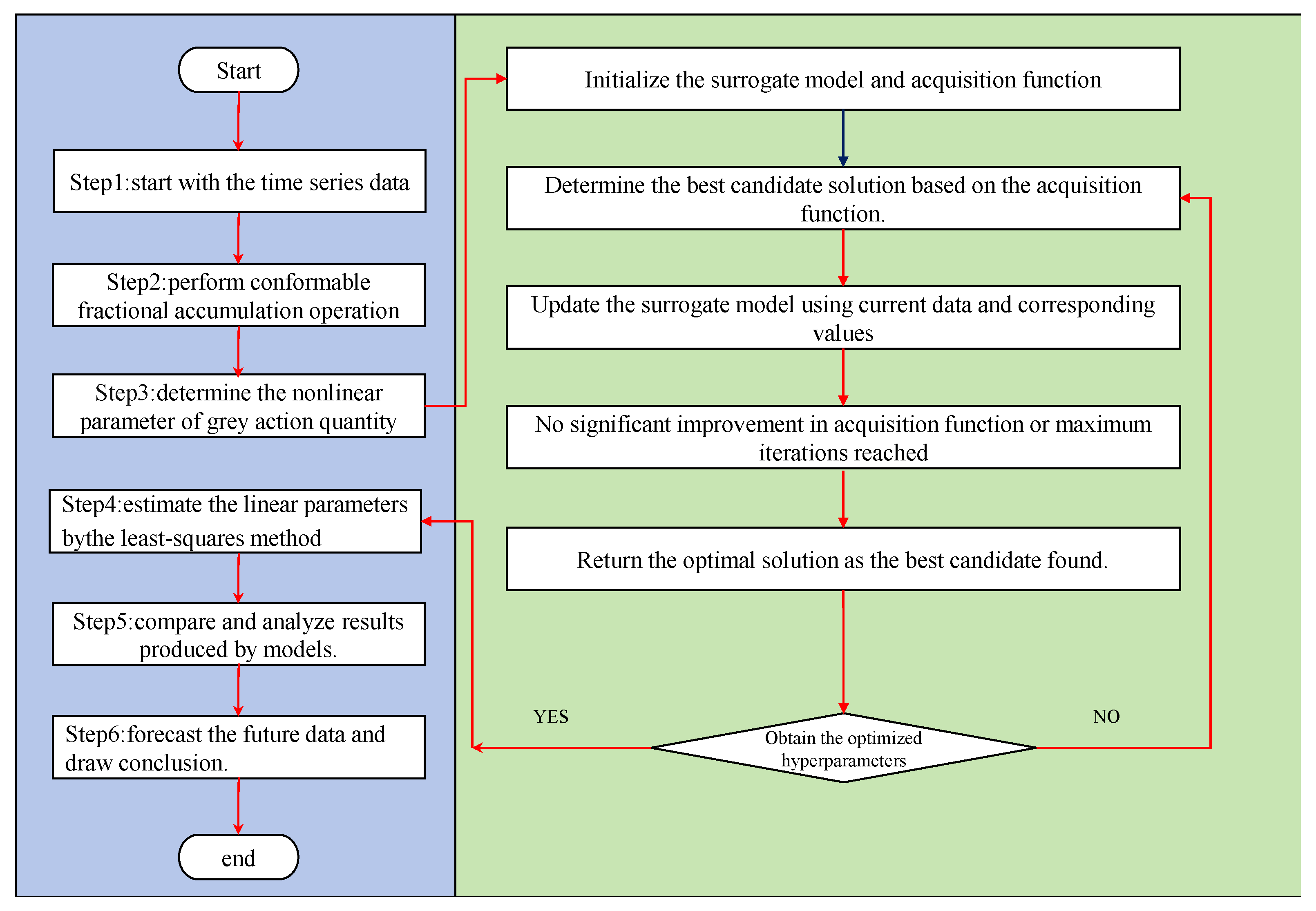
The overall computational steps of CFUKRNGM with Bayesian optimization algorithm are depicted in the flowchart shown in Figure 1. The implementation of the proposed algorithm is publicly available as open-source on GitHub 1

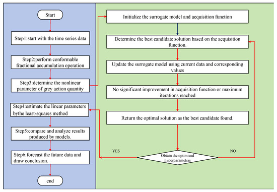
Figure 1. The flowchart of the conformable fractional order unbiased kernel regularized nonhomogeneous grey model.

5. Numerical Experiment

This section employs four publicly available real-world datasets to verify the superiority of the CFUKRNGM model. The models used for comparison are conformable fractional grey system(abbreviated as CFGM) [22], fractional grey system (abbreviated as FGM) [47], kernel regularized nonhomogeneous grey model (abbreviated as KRNGM) [29], grey model (abbreviated as GM) [9], discrete grey forecasting model (abbreviated as DGM) [48], self-adaptive intelligence grey model(abbreviated as SAIGM) [49], time-delayed grey model(abbreviated as TDGM) [50], nonlinear grey model(abbreviated as NGM) [51], and autoregressive grey model(abbreviated as ARGM) [52]. For the grey models with hyperparameters, namely CFUKRNGM, KRNGM, FGM, and CFGM, the Bayesian optimization algorithm is uniformly applied to optimize the hyperparameters. Table 1 briefly summarizes the basic information of each dataset. The four datasets are all sourced from the Energy Institute Statistical Review of World Energy 2.

Table 1. The information of the four datasets and the partitioning.

NO.	Name	Total	Modeling	Prediction
Case 1	China’s Oil Production	20 Months	From 1 to 15	From 16 to 20
Case 2	Carbon Dioxide Emissions from Energy	From 2004 to 2023	From 2004 to 2018	From 2019 to 2023
Case 3	Coal Production	From 2004 to 2023	From 2004 to 2018	From 2019 to 2023
Case 4	Electricity Generation from Gas	From 2004 to 2023	From 2004 to 2018	From 2019 to 2023

5.1. Evaluation Metrics

To evaluate and compare the effectiveness of various models, this study employs multiple performance indicators, including root mean squared error (RMSE), mean absolute error (MAE), normalized RMSE (NRMSE), mean absolute percentage error (MAPE), root mean squared percentage error (RMSPE), mean squared error (MSE), index of agreement (IA), and Theil’s U statistics (U1 and U2). These indicators comprehensively reflect both fitting and forecasting abilities of the CFUKRNGM model. The detailed mathematical definitions are provided in Table 2.

Table 2. The nine evaluation metrics.

Evaluation Metrics	Mathematical Formula
RMSE	${\left({\displaystyle \frac{1}{v}}{\sum }_{m=1}^v{\left(x^{\left(0\right)}\left(m\right)-{\widehat{x}}^{\left(0\right)}\left(m\right)\right)}^2\right)}^{0.5}$
MAE	${\displaystyle \frac{1}{v}}{\sum }_{m=1}^v\left|x^{\left(0\right)}\left(m\right)-{\widehat{x}}^{\left(0\right)}\left(m\right)\right|$
NRMSE	$\left({\displaystyle \frac{1}{\overline{x}}}\sqrt{{\displaystyle \frac{1}{v}}{\sum }_{m=1}^v{\left(x^{\left(0\right)}\left(m\right)-{\widehat{x}}^{\left(0\right)}\left(m\right)\right)}^2}\right)\times 100$
MAPE	${\displaystyle \frac{1}{v}}{\sum }_{m=1}^v\left({\displaystyle \frac{\left|x^{\left(0\right)}\left(m\right)-{\widehat{x}}^{\left(0\right)}\left(m\right)\right|}{\left|x^{\left(0\right)}\left(m\right)\right|}}\right)\times 100$
RMSPE	${\left({\displaystyle \frac{1}{v}}{\sum }_{m=1}^v{\left({\displaystyle \frac{\left(x^{\left(0\right)}\left(m\right)-{\widehat{x}}^{\left(0\right)}\left(m\right)\right)}{x^{\left(0\right)}\left(m\right)}}\right)}^2\right)}^{0.5}\times 100$
MSE	${\displaystyle \frac{1}{v}}{\sum }_{m=1}^v{\left(x^{\left(0\right)}\left(m\right)-{\widehat{x}}^{\left(0\right)}\left(m\right)\right)}^2$
IA	$1-{\displaystyle \frac{{\sum }_{m=1}^v{\left(x^{\left(0\right)}\left(m\right)-{\widehat{x}}^{\left(0\right)}\left(m\right)\right)}^2}{{\sum }_{m=1}^v{\left(\left|x^{\left(0\right)}\left(m\right)-\overline{x}\right|+\left|{\widehat{x}}^{\left(0\right)}\left(m\right)-\overline{x}\right|\right)}^2}}$
U1	${\left({\sum }_{m=1}^v{\left(x^{\left(0\right)}\left(m\right)-{\widehat{x}}^{\left(0\right)}\left(m\right)\right)}^2\right)}^{0.5}{\left({\left({\sum }_{m=1}^v{x}^{\left(0\right)}{\left(m\right)}^2\right)}^{0.5}+{\left({\sum }_{m=1}^v{\widehat{x}}^{\left(0\right)}{\left(m\right)}^2\right)}^{0.5}\right)}^{-1}$
U2	${\left({\sum }_{m=1}^v{\left(x^{\left(0\right)}\left(m\right)-{\widehat{x}}^{\left(0\right)}\left(m\right)\right)}^2\right)}^{0.5}{\left({\sum }_{m=1}^v{x}^{\left(0\right)}{\left(m\right)}^2\right)}^{-0.5}$

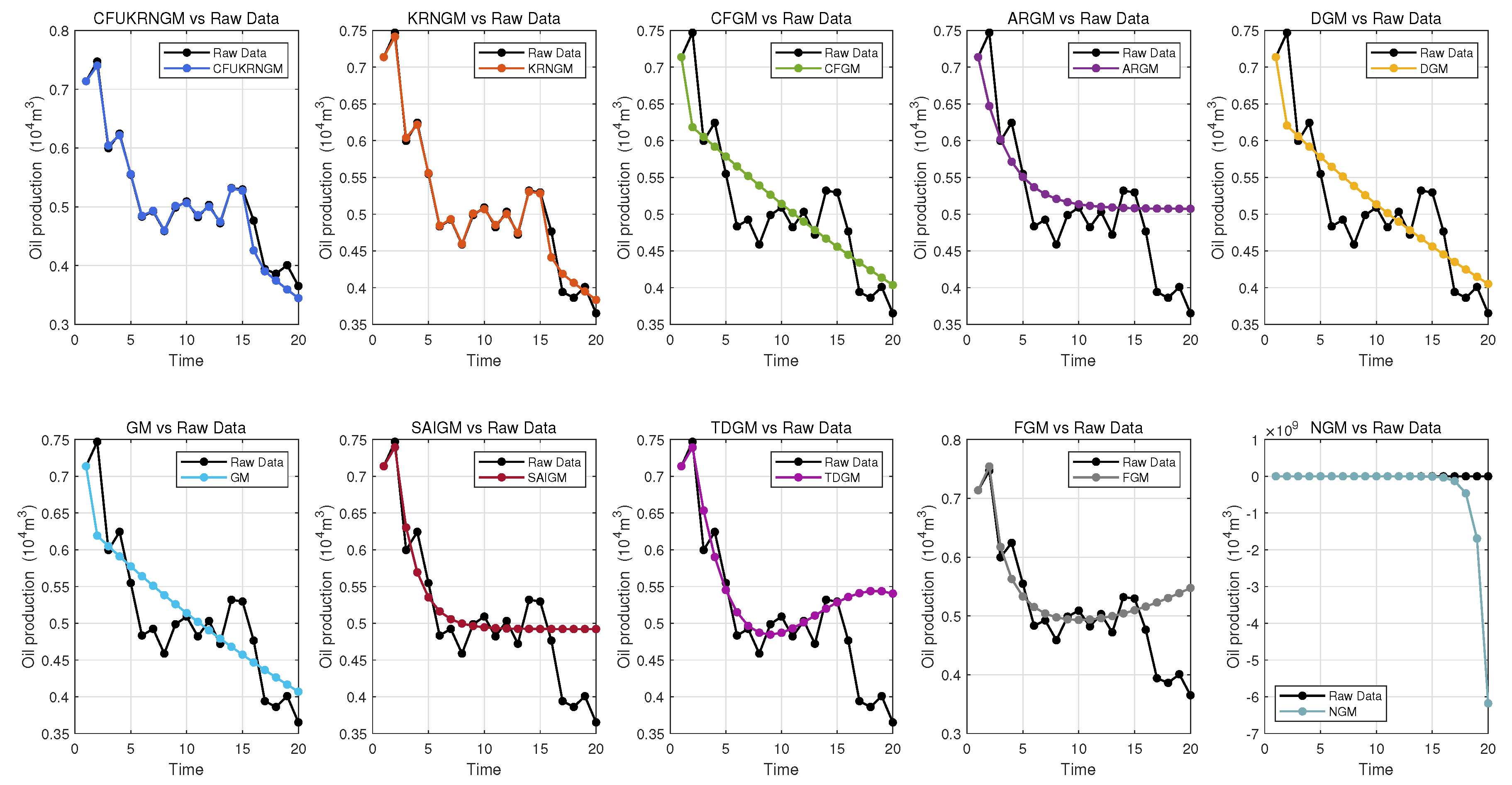
5.2. Case 1: Forecasting Oil Production in Block L

In this scenario, the CFUKRNGM model, along with other grey models for comparison, is utilized to simulate and predict oil production in Block L of the North China Oilfield (${10}^4{\mathrm{m}}^3$). Table 3 displays the oil production data spanning 20 months. Among these, the first 15 data points are used as the training set for model construction, while the remaining 5 are reserved for evaluating predictive performance. It is noteworthy that this dataset partitioning approach is consistent with the method adopted in [29].

Table 3. Raw data of monthly oil production (${10}^4{\mathrm{m}}^3$) of the block-L in North China oilfield.

Month	1	2	3	4	5	6	7	8	9	10
Oil production	0.7137	0.747	0.5997	0.6244	0.5548	0.4834	0.4924	0.4588	0.4988	0.5091
Month	11	12	13	14	15	16	17	18	19	20
Oil production	0.4822	0.5032	0.4721	0.532	0.5296	0.4765	0.3941	0.3862	0.4009	0.3652

Table 4 presents a comprehensive account of the predicted outcomes of the CFUKRNGM model alongside other grey models. The hyperparameters for the FGM, CFGM, KRNGM, and CFUKRNGM models were derived using the Bayesian optimization algorithm. In these models, hyperparameter adjustment is essential for improving model performance. The symbol $\gamma$ in the table represents the penalty parameter, utilized to control the model’s complexity and degree of fit. In the CFUKRNGM model, $\theta$ is a constant intricately linked to its structural attributes. $\alpha$ denotes the accumulation order of the FGM model, affecting the model’s fitting precision to the data. r denotes the accumulation order of the CFGM model, which dictates the model’s adaptability and fitting proficiency. $\sigma$ is the bandwidth of the radial basis function (RBF) kernel, which regulates the model’s smoothness and generalization capacity. The optimized hyperparameters yield the most effective configurations for the models during fitting and prediction, hence guaranteeing their efficiency and accuracy in practical applications.

Table 4. The oil production forecast results for the L block of the North China Oilfield.

Month	Oil Production	CFUKRNGM ($\mathit{\gamma }=97.8481$, $\mathit{\theta }=87.7075$, $\mathit{\alpha }=0.9809$, $\mathit{\sigma }=0.0815$)	ARGM	CFGM ($\mathit{\alpha }=0.9817$)	DGM	FGM ($\mathit{r}=1.3059$)	GM	KRNGM ($\mathit{\gamma }=99.9977$, $\mathit{\sigma }=0.0942$)	NGM	SAIGM	TDGM
1	0.7137	0.7137	0.7137	0.7137	0.7137	0.7137	0.7137	0.7137	$7.1370\times {10}^{-1}$	0.7137	0.7137
2	0.7470	0.7412	0.6471	0.6173	0.6206	0.7471	0.6192	0.7415	$3.5300\times {10}^{-2}$	0.7395	0.7392
3	0.5997	0.6040	0.6019	0.6056	0.6061	0.6175	0.6050	0.6038	$-1.2017\times {10}^0$	0.6303	0.6534
4	0.6244	0.6217	0.5714	0.5928	0.5919	0.5646	0.5910	0.6217	$-5.7169\times {10}^0$	0.5693	0.5902
5	0.5548	0.5558	0.5507	0.5797	0.5780	0.5353	0.5774	0.5558	$-2.2198\times {10}^1$	0.5353	0.5453
6	0.4834	0.4844	0.5367	0.5664	0.5645	0.5173	0.5641	0.4843	$-8.2359\times {10}^1$	0.5162	0.5151
7	0.4924	0.4932	0.5272	0.5531	0.5513	0.5061	0.5511	0.4931	$-3.0196\times {10}^2$	0.5056	0.4966
8	0.4588	0.4596	0.5207	0.5400	0.5383	0.4992	0.5384	0.4595	$-1.1035\times {10}^3$	0.4997	0.4871
9	0.4988	0.5010	0.5164	0.5270	0.5257	0.4954	0.5260	0.5008	$-4.0295\times {10}^3$	0.4964	0.4846
10	0.5091	0.5068	0.5134	0.5142	0.5134	0.4938	0.5138	0.5069	$-1.4710\times {10}^4$	0.4945	0.4871
11	0.4822	0.4855	0.5114	0.5016	0.5014	0.4941	0.5020	0.4854	$-5.3695\times {10}^4$	0.4935	0.4931
12	0.5032	0.5002	0.5101	0.4892	0.4897	0.4957	0.4904	0.5002	$-1.9600\times {10}^5$	0.4929	0.5013
13	0.4721	0.4747	0.5091	0.4771	0.4782	0.4985	0.4791	0.4747	$-7.1544\times {10}^5$	0.4926	0.5106
14	0.5320	0.5307	0.5085	0.4653	0.4670	0.5024	0.4681	0.5306	$-2.6115\times {10}^6$	0.4924	0.5199
15	0.5296	0.5281	0.5081	0.4537	0.4561	0.5071	0.4573	0.5283	$-9.5325\times {10}^6$	0.4923	0.5285
16	0.4765	0.4383	0.5078	0.4423	0.4454	0.5125	0.4467	0.4413	$-3.4796\times {10}^7$	0.4923	0.5358
17	0.3941	0.4131	0.5076	0.4312	0.4350	0.5187	0.4364	0.4188	$-1.2701\times {10}^8$	0.4922	0.5410
18	0.3862	0.4001	0.5075	0.4204	0.4248	0.5254	0.4264	0.4067	$-4.6362\times {10}^8$	0.4922	0.5438
19	0.4009	0.3876	0.5074	0.4098	0.4148	0.5328	0.4166	0.3949	$-1.6923\times {10}^9$	0.4922	0.5437
20	0.3652	0.3754	0.5073	0.3994	0.4051	0.5407	0.4070	0.3834	$-6.1772\times {10}^9$	0.4922	0.5404

Figure 2 presents a comparative assessment of the CFUKRNGM model against nine alternative grey prediction models in the simulation and forecasting of oil production in Block L of the North China Oilfield. An exhaustive evaluation of the prediction results reveals that the CFUKRNGM model demonstrates much superior predictive accuracy relative to its counterparts.

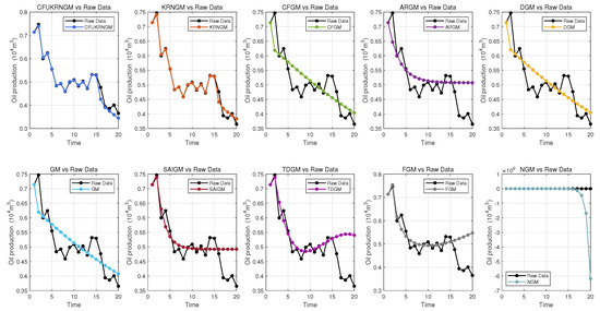
Figure 2. The performance of 10 grey models’ predictions in Case 1.

For the oil production data of Block L in the North China Oilfield, Table 5 presents the evaluation metrics for both fitting and prediction performance across different models. Among these, the CFUKRNGM model consistently outperforms others, demonstrating superior accuracy across multiple metrics. In terms of fitting performance, CFUKRNGM achieves the lowest RMSE of 0.0026 and the smallest MAE of 0.0022, highlighting its strong capability in reducing prediction errors.

Table 5. The computed evaluation metrics for the prediction results of 10 grey models in Case 1.

Metrics	CFUKRNGM	ARGM	CFGM	DGM	FGM	GM	KRNGM	NGM	SAIGM	TDGM
Fitting RMSE (↓)	0.0026	0.0403	0.0561	0.0547	0.0255	0.0547	0.0547	2.5592$\times {10}^6$	0.0273	0.0238
MAE (↓)	0.0022	0.0299	0.0421	0.0411	0.0201	0.0410	0.0410	8.7529$\times {10}^5$	0.0224	0.0180
NRMSE (↓)	0.4796	7.3630	10.2683	10.0119	4.6681	10.0114	10.0114	4.6808$\times {10}^8$	4.9895	4.3456
MAPE (↓)	0.3922	5.5111	7.7636	7.5837	3.8495	7.5684	7.5684	1.6643$\times {10}^8$	4.2266	3.4135
RMSPE (↓)	0.4536	7.0912	10.0954	9.8440	4.8004	9.8207	9.8207	4.8342$\times {10}^8$	5.1117	4.4707
MSE (↓)	0.0000	0.0016	0.0032	0.0030	0.0007	0.0030	0.0030	6.5495$\times {10}^{12}$	0.0007	0.0006
IA (↑)	0.9990	0.7737	0.5599	0.5816	0.9090	0.5817	0.5817	−9.1441$\times {10}^{14}$	0.8961	0.9212
U1 (↓)	0.0024	0.0364	0.0509	0.0496	0.0231	0.0496	0.0496	1.0000	0.0247	0.0214
U2 (↓)	0.0047	0.0728	0.1015	0.0989	0.0461	0.0989	0.0989	4.6257$\times {10}^6$	0.0493	0.0429
Prediction RMSE (↓)	0.0214	0.1097	0.0315	0.0344	0.1299	0.0354	0.0230	2.8724$\times {10}^9$	0.0955	0.1422
MAE (↓)	0.0189	0.1030	0.0297	0.0329	0.1214	0.0339	0.0209	1.6989$\times {10}^9$	0.0876	0.1364
NRMSE (↓)	5.2983	27.1047	7.7872	8.4996	32.1106	8.7605	5.6785	7.0998$\times {10}^{11}$	23.5976	35.1374
MAPE (↓)	4.5128	26.4543	7.4040	8.2577	31.2333	8.5461	5.0912	4.5463$\times {10}^{11}$	22.6392	34.8273
RMSPE (↓)	4.8874	28.5656	7.8880	8.7339	33.9029	9.0402	5.4627	7.8163$\times {10}^{11}$	24.9476	36.8284
MSE (↓)	0.0005	0.0120	0.0010	0.0012	0.0169	0.0013	0.0005	8.2508$\times {10}^{18}$	0.0091	0.0202
IA (↑)	0.6802	−7.3690	0.3092	0.1770	−10.7458	0.1257	0.6327	−5.7421$\times {10}^{21}$	−5.3434	−13.0645
U1 (↓)	0.0265	0.1200	0.0381	0.0414	0.1393	0.0425	0.0282	1.0000	0.1063	0.1501
U2 (↓)	0.0528	0.2699	0.0775	0.0846	0.3197	0.0872	0.0565	7.0688$\times {10}^9$	0.2349	0.3498

Note: ↑ indicates that a larger value is preferred (higher-is-better), while ↓ indicates that a smaller value is preferred (lower-is-better). The same convention applies to all subsequent tables.

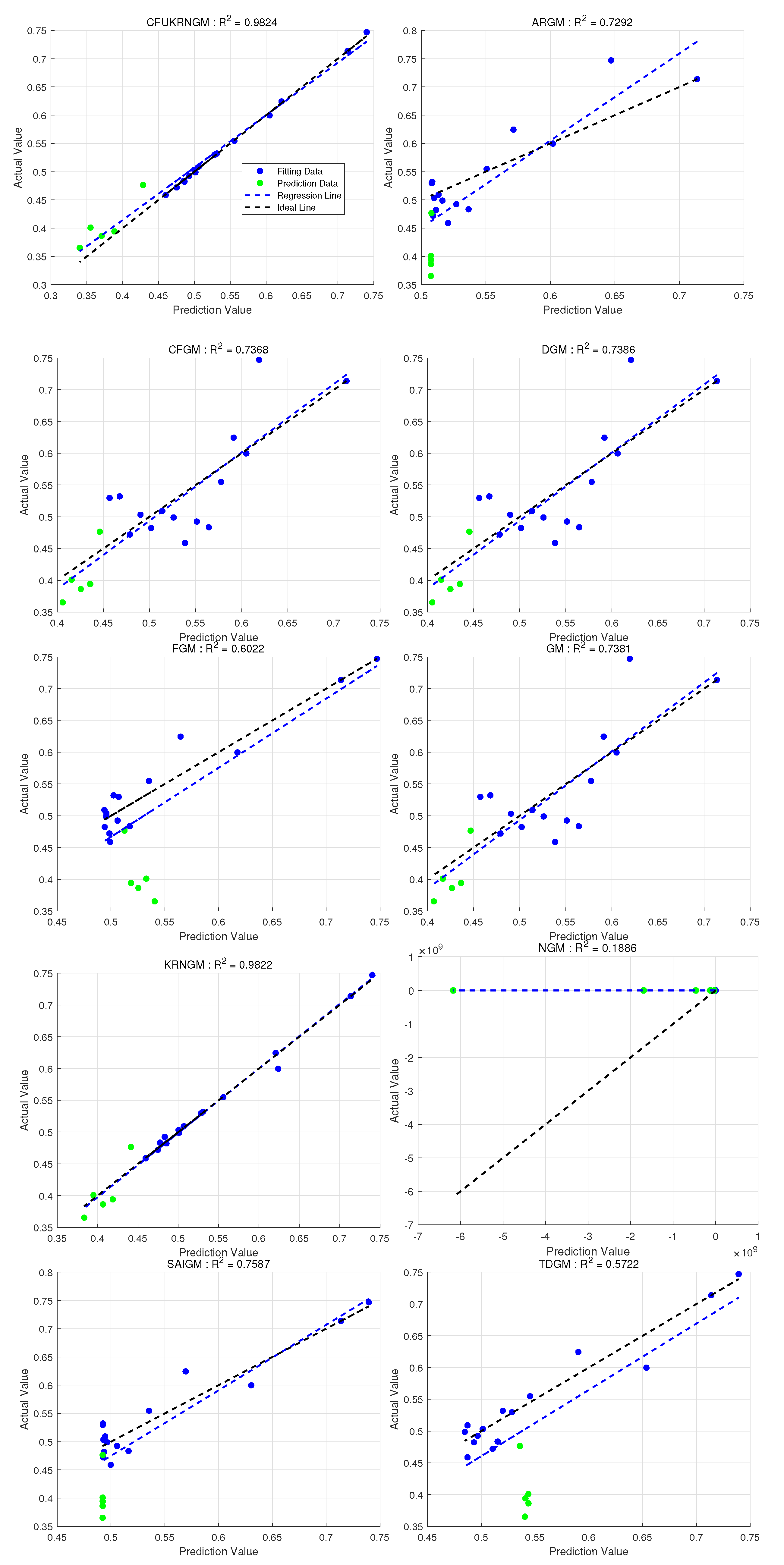
Figure 3 illustrates the detailed outcomes for all 10 models. The results clearly show that the majority of points predicted by CFUKRNGM closely align with the actual data, and the model achieves the highest overall R value. Therefore, in this validation case, CFUKRNGM proves to be the most effective model.

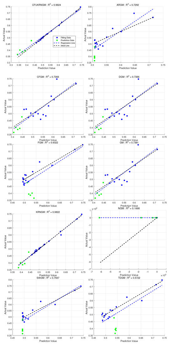
Figure 3. The regression performance of ten grey models in Case 1. $R^2$ represents the coefficient of determination between the raw data and the predicted values of the models (Overall).

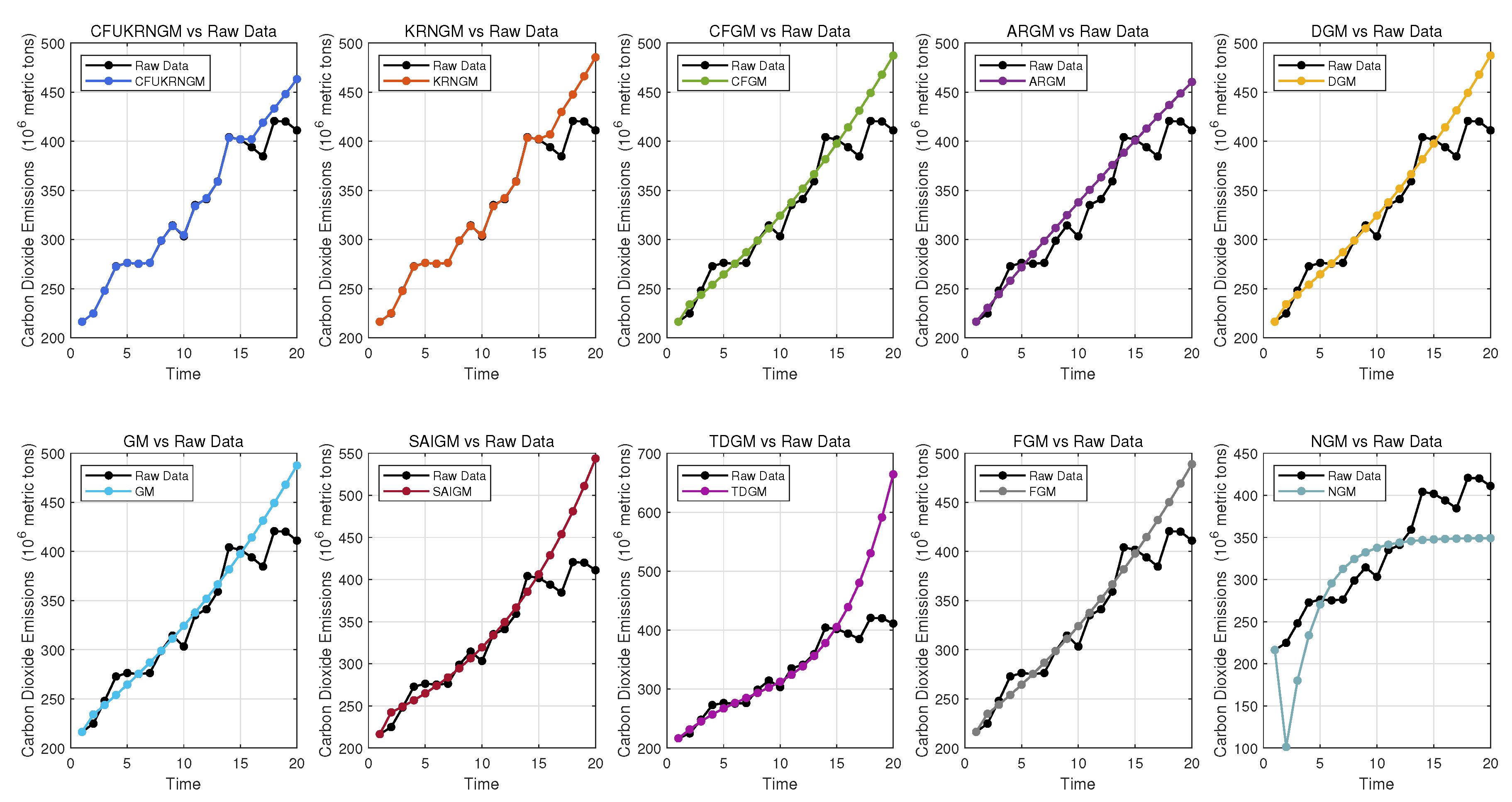
5.3. Case 2: Forecasting Carbon Dioxide Emissions in Turkey

Table 6 lists the carbon dioxide emission data for Turkey from 2004 to 2023. In this case, the hyperparameters of the FGM, CFGM, KRNGM, and CFUKRNGM models employed were meticulously tuned using the Bayesian optimization algorithm.

Table 6. Carbon dioxide emissions in Turkey from 2004 to 2023 (unit: million metric tons).

Year	2004	2005	2006	2007	2008	2009	2010	2011	2012	2013
Emission	216.4	224.8	248.0	272.8	276.3	275.3	276.3	298.8	314.4	303.3
Year	2014	2015	2016	2017	2018	2019	2020	2021	2022	2023
Emission	335.1	341.1	359.2	404.2	401.8	394.0	384.6	420.7	420.4	411.1

Simulation forecasts were conducted for Turkey’s carbon dioxide emissions data spanning from 2004 to 2023, and the optimized hyperparameters are detailed in Table 7. Furthermore, metrics for assessing the fitting and predictive performance of each model are systematically presented in Table 8. A comprehensive analysis of the data in Table 7 and Table 8 reveals that the CFUKRNGM model not only demonstrates superior performance in fitting historical carbon dioxide emission data of Turkey but also outperforms other models in predicting data beyond the sample range, thereby confirming its significant advantages in terms of robustness and predictive accuracy.

Table 7. The carbon dioxide emissions forecast results for Turkey from 2004 to 2023.

Year	Carbon Dioxide Emissions	CFUKRNGM ($\mathit{\gamma }=91.5762$, $\mathit{\theta }=29.3618$, $\mathit{\alpha }=0.8293$, $\mathit{\sigma }=0.0108$)	ARGM	CFGM ($\mathit{\alpha }=0.9953$)	DGM	FGM ($\mathit{r}=1.0028$)	GM	KRNGM ($\mathit{\gamma }=99.9993$, $\mathit{\sigma }=0.0185$)	NGM	SAIGM	TDGM
2004	216.4	216.4000	216.4000	216.4000	216.4000	216.4000	216.4000	216.4000	216.4000	216.4000	216.4000
2005	224.8	224.9704	230.4513	233.9799	234.1835	234.5877	234.0667	224.9704	101.2048	242.3103	231.4886
2006	248	247.6885	244.3601	243.7709	243.9169	244.0031	243.8046	247.6885	179.9963	249.1465	245.0977
2007	272.8	272.4826	258.1279	253.9461	254.0547	253.9683	253.9477	272.4826	233.7770	256.6431	256.8477
2008	276.3	276.2969	271.7562	264.5313	264.6139	264.4261	264.5127	276.2969	270.4861	264.8639	267.1155
2009	275.3	275.4745	285.2463	275.5482	275.6120	275.3669	275.5173	275.4745	295.5425	273.8790	276.3172
2010	276.3	276.3359	298.5996	287.0170	287.0672	286.7962	286.9797	276.3359	312.6453	283.7650	284.9122
2011	298.8	298.8901	311.8176	298.9578	298.9985	298.7263	298.9189	298.8901	324.3191	294.6061	293.4076
2012	314.4	313.8068	324.9015	311.3912	311.4257	311.1730	311.3549	313.8068	332.2873	306.4946	302.3634
2013	303.3	304.6087	337.8528	324.3383	324.3694	324.1547	324.3082	304.6087	337.7262	319.5316	312.3980
2014	335.1	333.8528	350.6728	337.8208	337.8511	337.6913	337.8005	333.8528	341.4386	333.8282	324.1941
2015	341.1	342.0929	363.3629	351.8612	351.8931	351.8044	351.8541	342.0929	343.9726	349.5059	338.5053
2016	359.2	358.7860	375.9242	366.4830	366.5188	366.5171	366.4923	358.7860	345.7022	366.6983	356.1640
2017	404.2	403.4932	388.3583	381.7105	381.7523	381.8534	381.7396	403.4932	346.8828	385.5516	378.0889
2018	401.8	402.3295	400.6663	397.5689	397.6190	397.8388	397.6211	402.3295	347.6886	406.2263	405.2947
2019	394	406.9946	412.8495	414.0846	414.1452	414.5000	414.1634	406.9946	348.2386	428.8985	438.9014
2020	384.6	429.8464	424.9092	431.2850	431.3582	431.8648	431.3939	429.8464	348.6140	453.7610	480.1458
2021	420.7	447.6455	436.8466	449.9624	449.2866	449.9624	449.3413	447.6455	348.8703	481.0254	530.3934
2022	420.4	466.1816	448.6630	467.8548	467.9602	468.8233	468.0353	466.1816	349.0452	510.9239	591.1520
2023	411.1	485.4853	460.3596	487.2848	487.4099	488.4791	487.5071	485.4853	349.1646	543.7110	664.0860

Table 8. The computed evaluation metrics for the prediction results of 10 grey models in Case 2.

Metrics	CFUKRNGM	ARGM	CFGM	DGM	FGM	GM	KRNGM	NGM	SAIGM	TDGM
Fitting RMSE (↓)	0.5915	15.5371	11.1719	11.1371	11.1191	11.1374	0.6231	46.0347	10.3180	10.1745
MAE (↓)	0.4266	12.6907	8.4843	8.4474	8.4115	8.4371	0.4597	33.6663	8.2478	7.8018
NRMSE (↓)	0.1951	5.1246	3.6848	3.6733	3.6674	3.6734	0.2055	15.1836	3.4032	3.3559
MAPE (↓)	0.1345	4.1206	2.7748	2.7672	2.7585	2.7637	0.1421	11.9358	2.7632	2.5084
RMSPE (↓)	0.1851	5.0301	3.6197	3.6181	3.6194	3.6180	0.1909	17.9738	3.5653	3.1263
MSE (↓)	0.3499	241.4020	124.8118	124.0343	123.6341	124.0410	0.3883	2119.1920	106.4605	103.5211
IA(↑)	0.9999	0.9205	0.9589	0.9591	0.9593	0.9591	0.9999	0.3019	0.9649	0.9659
U1(↓)	0.0010	0.0249	0.0181	0.0181	0.0181	0.0181	0.0010	0.0760	0.0167	0.0166
U2(↓)	0.0019	0.0504	0.0363	0.0361	0.0361	0.0361	0.0020	0.1494	0.0335	0.0330
Prediction RMSE (↓)	9.4834	19.0895	19.0895	27.6822	28.0097	27.7173	26.5472	34.1332	48.5939	88.0666
MAE (↓)	4.2268	10.1885	10.1885	14.6240	14.8058	14.6427	13.6902	19.1245	25.8347	44.9252
NRMSE (↓)	2.3349	4.7000	4.7000	6.8156	6.8962	6.8242	6.5361	8.4039	11.9642	21.6827
MAPE (↓)	1.0500	2.5205	2.5205	3.5961	3.6405	3.6006	3.3635	4.6723	6.3313	10.9646
RMSPE (↓)	2.3620	4.7346	4.7346	6.7954	6.8750	6.8039	6.5131	8.2826	11.8650	21.3910
MSE (↓)	89.9352	364.4101	364.4101	766.3015	784.5446	768.2483	704.7523	1165.0730	2361.3699	7755.7298
IA(↑)	-0.2832	−4.1995	−4.1995	−9.9337	−10.1940	−9.9615	−9.0555	−15.6234	−32.6924	−109.6600
U1(↓)	0.0199	0.0392	0.0392	0.0559	0.0566	0.0560	0.0538	0.0783	0.0944	0.1600
U2(↓)	0.0404	0.0814	0.0814	0.1180	0.1194	0.1181	0.1131	0.1455	0.2071	0.3753

Figure 4 and Figure 5 respectively illustrate the forecasting outcomes of various grey prediction models. The analysis clearly indicates that the CFUKRNGM model outperforms the others in predictive accuracy. Notably, the coefficient of determination $R^2$ for CFUKRNGM reaches 0.982, exhibiting only a slight deviation from the theoretical optimal value of 1, which strongly validates its superior predictive performance and generalization ability.

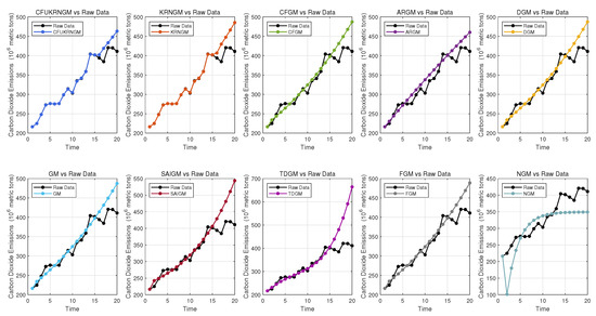
Figure 4. The performance of 10 grey models’ predictions in Case 2.

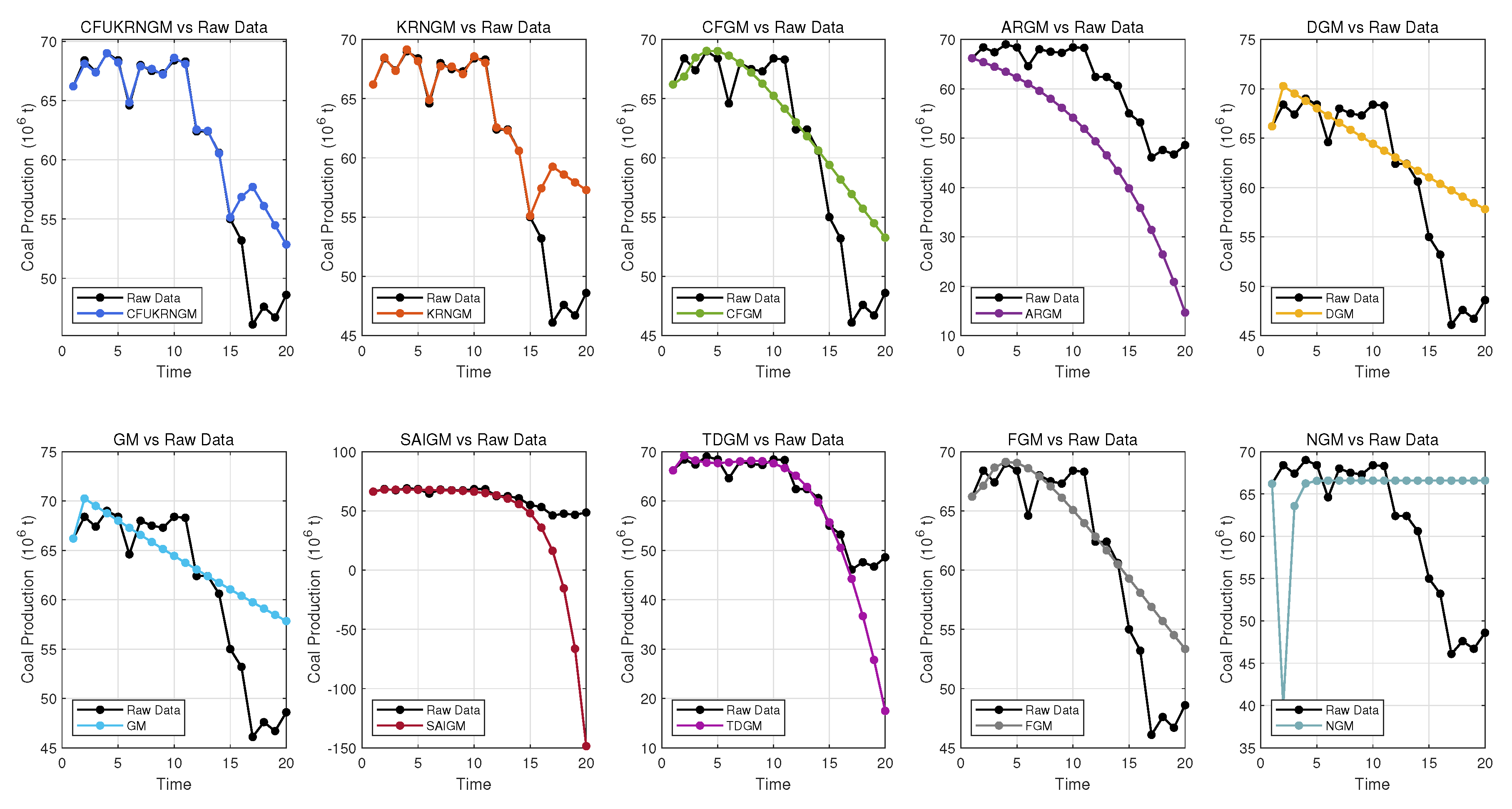
5.4. Case 3: Forecasting Coal Production of Canada

In this case, grey models are used to simulate and predict coal production. The data in Table 9 represents Canada’s coal production from 2004 to 2023.

Table 9. Coal production of Canada from 2004 to 2023 (unit: ${10}^6\mathrm{tonnes}$).

Year	2004	2005	2006	2007	2008	2009	2010	2011	2012	2013
Production	66.2	68.4	67.4	69.0	68.4	64.6	68.0	67.5	67.3	68.4
Year	2014	2015	2016	2017	2018	2019	2020	2021	2022	2023
Production	68.3	62.4	62.4	60.6	55.0	53.2	46.1	47.6	46.7	48.6

The prediction results of the 10 grey models are summarized in Table 10. The hyperparameter optimization results for the FGM, CFGM, KRNGM, and CFUKRNGM models are also provided in Table 10. Clearly, the CFUKRNGM model exhibits the best predictive performance for out-of-sample data, demonstrating superior generalization ability and better capturing future trends.

Table 10. The coal production forecast results for Canada from 2004 to 2023.

Year	Coal Production	CFUKRNGM ($\mathit{\gamma }=90.9921$, $\mathit{\theta }=74.8937$, $\mathit{\alpha }=0.6321$, $\mathit{\sigma }=0.0106$)	ARGM	CFGM ($\mathit{\alpha }=0.8691$)	DGM	FGM ($\mathit{r}=0.8796$)	GM	KRNGM ($\mathit{\gamma }=99.9935$, $\mathit{\sigma }=0.1159$)	NGM	SAIGM	TDGM
2004	66.2	66.2000	66.2000	66.2000	66.2000	66.2000	66.2000	66.2000	66.2000	66.2000	66.2000
2005	68.4	68.2216	65.3821	66.8776	70.2773	67.0168	70.2553	68.4647	39.8600	67.9255	69.2202
2006	67.4	67.3750	64.4665	68.4679	69.5186	68.6201	69.5003	67.3433	63.5703	67.9008	68.2143
2007	69	69.1399	63.4417	69.0294	68.7681	69.1478	68.7534	69.1417	66.2411	67.8611	67.7561
2008	68.4	68.1894	62.2945	69.0133	68.0257	69.0778	68.0145	68.1654	66.5420	67.7971	67.6783
2009	64.6	64.9392	61.0104	68.6314	67.2914	68.6395	67.2836	64.8975	66.5759	67.6940	67.8204
2010	68	67.8849	59.5729	68.0019	66.5649	67.9578	66.5605	67.7324	66.5797	67.5278	68.0290
2011	67.5	67.7206	57.9639	67.1974	65.8463	67.1086	65.8452	67.7056	66.5802	67.2599	68.1567
2012	67.3	67.1785	56.1628	66.2665	65.1355	66.1412	65.1376	67.0754	66.5802	66.8283	68.0625
2013	68.4	68.6506	54.1467	65.2429	64.4323	65.0893	64.4375	68.5674	66.5802	66.1327	67.6114
2014	68.3	68.0281	51.8898	64.1512	63.7367	63.9773	63.7450	68.0254	66.5802	65.0118	66.6737
2015	62.4	62.5462	49.3636	63.0096	63.0486	62.8229	63.0600	62.5710	66.5802	63.2054	65.1253
2016	62.4	62.3902	46.5358	61.8321	62.3680	61.6398	62.3823	62.3121	66.5802	60.2944	62.8475
2017	60.6	60.5245	43.3704	60.6299	61.6947	60.4382	61.7119	60.5895	66.5802	55.6033	59.7262
2018	55	55.0397	39.8272	59.4114	61.0286	59.2263	61.0487	55.1032	66.5802	48.0435	55.6522
2019	53.2	53.4582	35.8609	58.1837	60.3698	58.0107	60.3926	57.4318	66.5802	35.8609	50.5211
2020	46.1	51.1536	31.4212	56.9523	59.7181	56.7963	59.7436	59.2572	66.5802	16.2286	44.2325
2021	47.6	49.0311	26.4514	55.7218	59.0734	55.5873	59.1015	58.5940	66.5802	−15.4090	36.6903
2022	46.7	46.9494	20.8884	54.4960	58.4356	54.3870	58.4664	57.9383	66.5802	−66.3933	27.8027
2023	48.6	44.9155	14.6613	53.2779	57.8048	53.1982	57.8381	57.2900	66.5802	−148.5548	17.4813

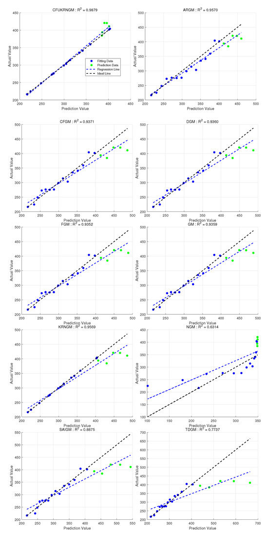
Figure 5. The regression performance of ten grey models in Case 2. $R^2$ represents the coefficient of determination between the raw data and the predicted values of the models (Overall).

Figure 5. The regression performance of ten grey models in Case 2. $R^2$ represents the coefficient of determination between the raw data and the predicted values of the models (Overall).

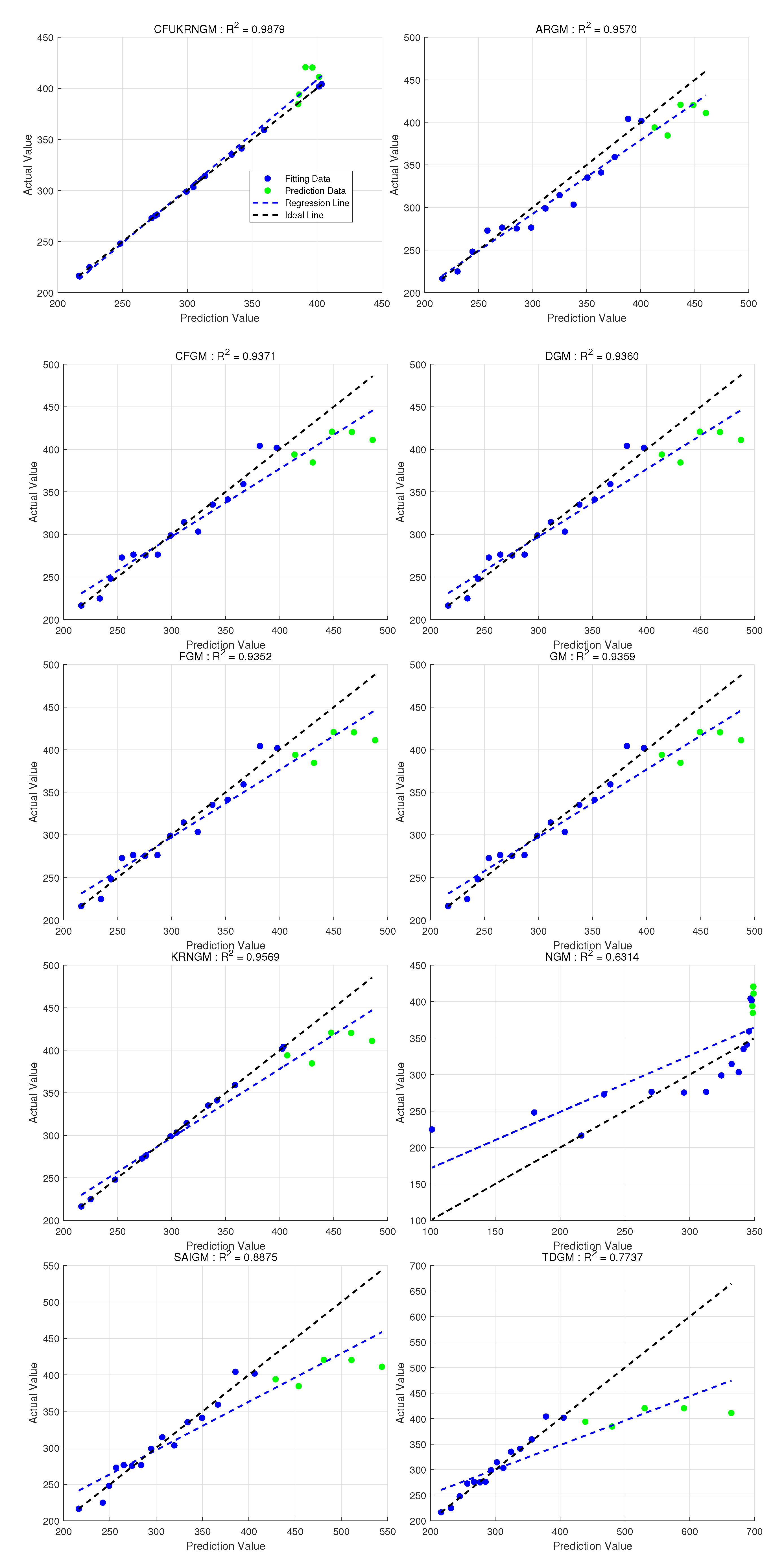
Figure 6 and Figure 7 present the prediction results of the 10 models. It is evident that most of the points generated by CFUKRNGM closely match the raw data, while the results from the other models are noticeably inferior, and CFUKRNGM achieves the highest overall $R^2$value. Hence, in this validation case, CFUKRNGM outperforms all the other models.

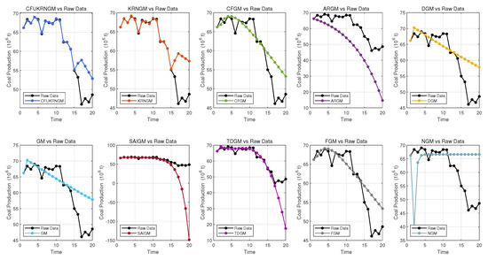
Figure 6. The performance of 10 grey models’ predictions in Case 3.

Table 11 presents the evaluation of the prediction results of the 10 grey models for Canada’s coal production. Based on these metric values, the KRNGM and CFUKRNGM models exhibit smaller fitting errors, indicating a better ability to capture historical data trends. However, the CFUKRNGM model achieves lower prediction errors for future data, making it more accurate in forecasting future trends.

Table 11. The computed evaluation metrics for the prediction results of 10 grey models in Case 3.

Metrics	CFUKRNGM	ARGM	CFGM	DGM	FGM	GM	KRNGM	NGM	SAIGM	TDGM
Fitting RMSE (↓)	0.1887	10.9724	2.1378	2.5750	2.1580	2.5750	0.1801	8.4009	2.6659	1.3385
MAE (↓)	0.1505	9.4848	1.4354	1.9254	1.4844	1.9256	0.1539	4.7655	1.8277	1.0255
NRMSE (↓)	0.2876	16.7279	3.2591	3.9257	3.2900	3.9257	0.2746	12.8076	4.0643	2.0405
MAPE (↓)	0.2256	14.7713	2.2416	3.0036	2.3109	3.0044	0.2324	7.4134	2.9465	1.5764
RMSPE (↓)	0.2825	17.3293	3.4052	4.1534	3.4125	4.1558	0.2707	12.7990	4.5000	2.0723
MSE (↓)	0.0356	120.3936	4.5701	6.6307	4.6571	6.6306	0.0324	70.5751	7.1072	1.7915
IA (↑)	0.9975	−7.3195	0.6842	0.5418	0.6782	0.5418	0.9978	−3.8769	0.5089	0.8762
U1 (↓)	0.0014	0.0897	0.0163	0.0196	0.0164	0.0196	0.0014	0.0643	0.0205	0.0102
U2 (↓)	0.0029	0.1670	0.0325	0.0392	0.0328	0.0392	0.0027	0.1279	0.0406	0.0204
Prediction RMSE (↓)	3.3936	23.5858	7.6118	10.8715	7.4209	10.8991	10.1361	18.3152	106.6051	17.0597
Prediction MAE (↓)	2.7258	22.5834	7.2649	10.6403	7.0669	10.6684	9.6623	18.1402	84.0935	13.0944
Prediction NRMSE (↓)	7.0057	48.6907	15.7139	22.4432	15.3197	22.5003	20.9251	37.8100	220.0765	35.2183
Prediction MAPE (↓)	5.6870	46.7934	15.2135	22.2381	14.8042	22.2965	20.3074	37.8034	175.5199	27.3004
Prediction RMSPE (↓)	7.0590	48.9523	16.1097	22.9149	15.7136	22.9725	21.4948	38.4112	221.8091	35.5089
Prediction MSE (↓)	11.5163	556.2899	57.9397	118.1896	55.0691	118.7912	102.7406	335.4455	11364.6431	291.0341
Prediction IA (↑)	−0.8055	−86.2146	−8.0837	−17.5297	−7.6337	−17.6240	−15.1076	−51.5909	−1780.7389	−44.6281
Prediction U1 (↓)	0.0355	0.3127	0.0730	0.1010	0.0713	0.1013	0.0951	0.1591	0.8619	0.1990
Prediction U2 (↓)	0.0700	0.4863	0.1569	0.2241	0.1530	0.2247	0.2090	0.3776	2.1978	0.3517

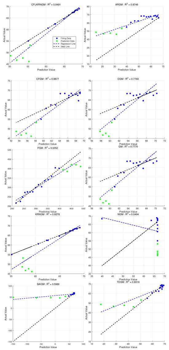
Figure 7. The regression performance of ten grey models in Case 3. $R^2$ represents the coefficient of determination between the raw data and the predicted values of the models (Overall).

Figure 7. The regression performance of ten grey models in Case 3. $R^2$ represents the coefficient of determination between the raw data and the predicted values of the models (Overall).

5.5. Case 4: Forecasting Natural Gas Electricity Generation in U.S.

This case study employs grey models to simulate and predict natural gas electricity generation in the United States. The original statistical data on U.S. natural gas electricity generation from 2003 to 2023 is provided in Table 12. Table 13 summarizes the simulation and forecasting results across ten grey models; the optimized hyperparameters for the FGM, CFGM, KRNGM, and CFUKRNGM models are also detailed in Table 13.

Table 12. Natural gas electricity generation in the U.S from 2004 to 2023 (unit: Terawatt-hours).

Year	2004	2005	2006	2007	2008	2009	2010	2011	2012	2013
Generation	763.5	818.2	877.9	964.1	949.4	990.3	1062.0	1090.0	1318.2	1209.5
Year	2014	2015	2016	2017	2018	2019	2020	2021	2022	2023
Generation	1211.4	1435.1	1483.1	1395.4	1582.6	1708.1	1749.2	1698.1	1814.1	1937.7

Table 13. The electricity generation from gas forecast results for United States from 2004 to 2023.

Year	Electricity Generation	CFUKRNGM ($\mathit{\gamma }=97.6935$, $\mathit{\theta }=1.7422$) ($\mathit{\alpha }=0.7297$, $\mathit{\sigma }=0.2376$)	ARGM	CFGM ($\mathit{\alpha }=0.9589$)	DGM	FGM ($\mathit{r}=0.9729$)	GM	KRNGM ($\mathit{\gamma }=99.9965$, $\mathit{\sigma }=0.0308$)	NGM	SAIGM	TDGM
2004	763.5	763.5000	763.5000	763.5000	763.5000	763.5000	763.5000	763.5000	763.5000	763.5000	763.5000
2005	818.2	817.7287	841.7479	830.5556	842.6334	829.8193	841.8743	818.2038	349.0039	824.7984	831.7717
2006	877.9	877.7716	915.5636	878.0895	883.8792	878.3379	883.1496	877.1191	616.2725	872.6037	874.5524
2007	964.1	963.6613	985.1980	925.2792	927.1440	925.7748	926.4486	963.7392	816.1849	921.6595	920.5546
2008	949.4	949.3191	1050.8881	973.2401	972.5265	973.7472	971.8704	949.2829	965.7162	971.9986	969.5025
2009	990.3	993.4805	1112.8573	1022.5145	1020.1304	1022.9408	1019.5191	992.9757	1077.5631	1023.6545	1021.1078
2010	1062	1056.9566	1171.3163	1073.4344	1070.0645	1073.7430	1069.5039	1056.9827	1161.2228	1076.6616	1075.0693
2011	1090	1098.1911	1226.4639	1126.2379	1122.4428	1126.4179	1121.9394	1097.5235	1223.7988	1131.0554	1131.0718
2012	1318.2	1305.7601	1278.4878	1181.1166	1177.3849	1181.1711	1176.9457	1305.0361	1270.6047	1186.8720	1188.7860
2013	1209.5	1221.6999	1327.5648	1238.2375	1235.4689	1238.1781	1295.1811	1222.7420	1305.6147	1244.1488	1247.8675
2014	1211.4	1204.9476	1373.8620	1297.7546	1295.4689	1297.5990	1295.1811	1204.0768	1331.8016	1302.9238	1307.9563
2015	1435.1	1438.0868	1417.5367	1359.8157	1358.8804	1359.5862	1358.6811	1437.4796	1351.3890	1363.2364	1368.6760
2016	1483.1	1478.2894	1458.7374	1424.5659	1425.3958	1424.2892	1425.2943	1478.9293	1366.0400	1425.1267	1429.6330
2017	1395.4	1403.5242	1497.6044	1492.1507	1495.1671	1491.8571	1495.1734	1403.8016	1376.9987	1488.6359	1490.4160
2018	1582.6	1575.7005	1534.2699	1562.7174	1568.3537	1562.4413	1568.4786	1574.9704	1385.1957	1553.8065	1550.5948
2019	1708.1	1738.6849	1568.8584	1636.4168	1645.1226	1636.1961	1645.3778	1759.9234	1391.3269	1620.6819	1609.7199
2020	1749.2	1720.6003	1601.4878	1713.4036	1725.6492	1713.2805	1726.0471	1770.3782	1395.9129	1689.3067	1667.3209
2021	1698.1	1796.0167	1632.2688	1793.8378	1810.1175	1793.8587	1810.6715	1862.4934	1399.3432	1759.7266	1722.9065
2022	1814.1	1874.1510	1661.3064	1877.8849	1898.7205	1878.1007	1899.4449	1959.4017	1401.9090	1831.9886	1775.9628
2023	1937.7	1955.1344	1688.6991	1965.7168	1991.6604	1966.1832	1992.5706	2061.3523	1403.8281	1906.1410	1825.9526

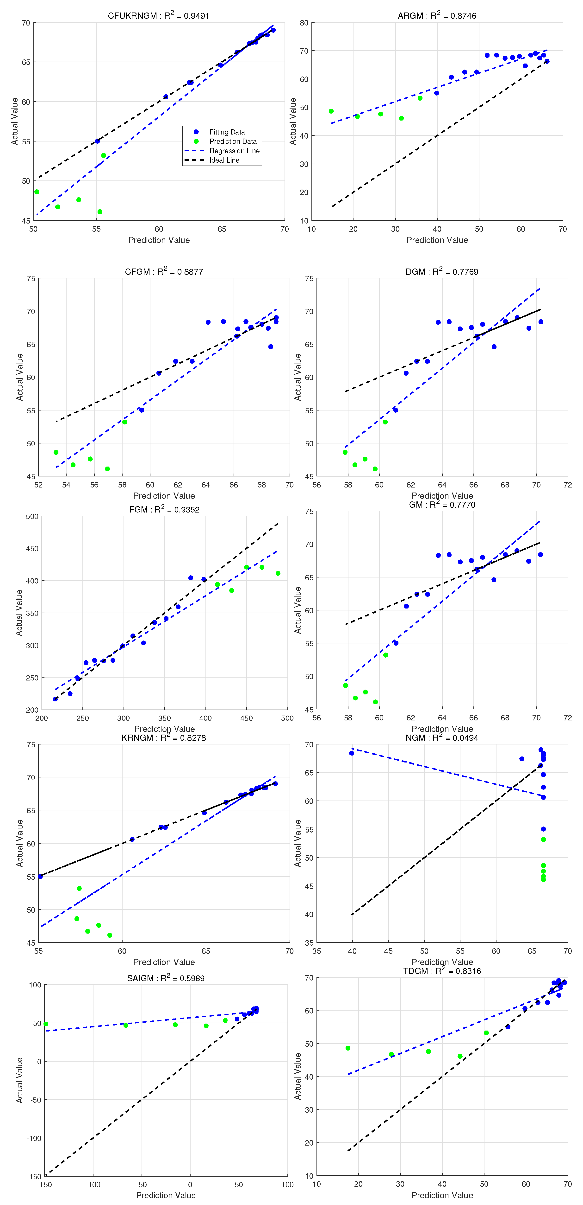
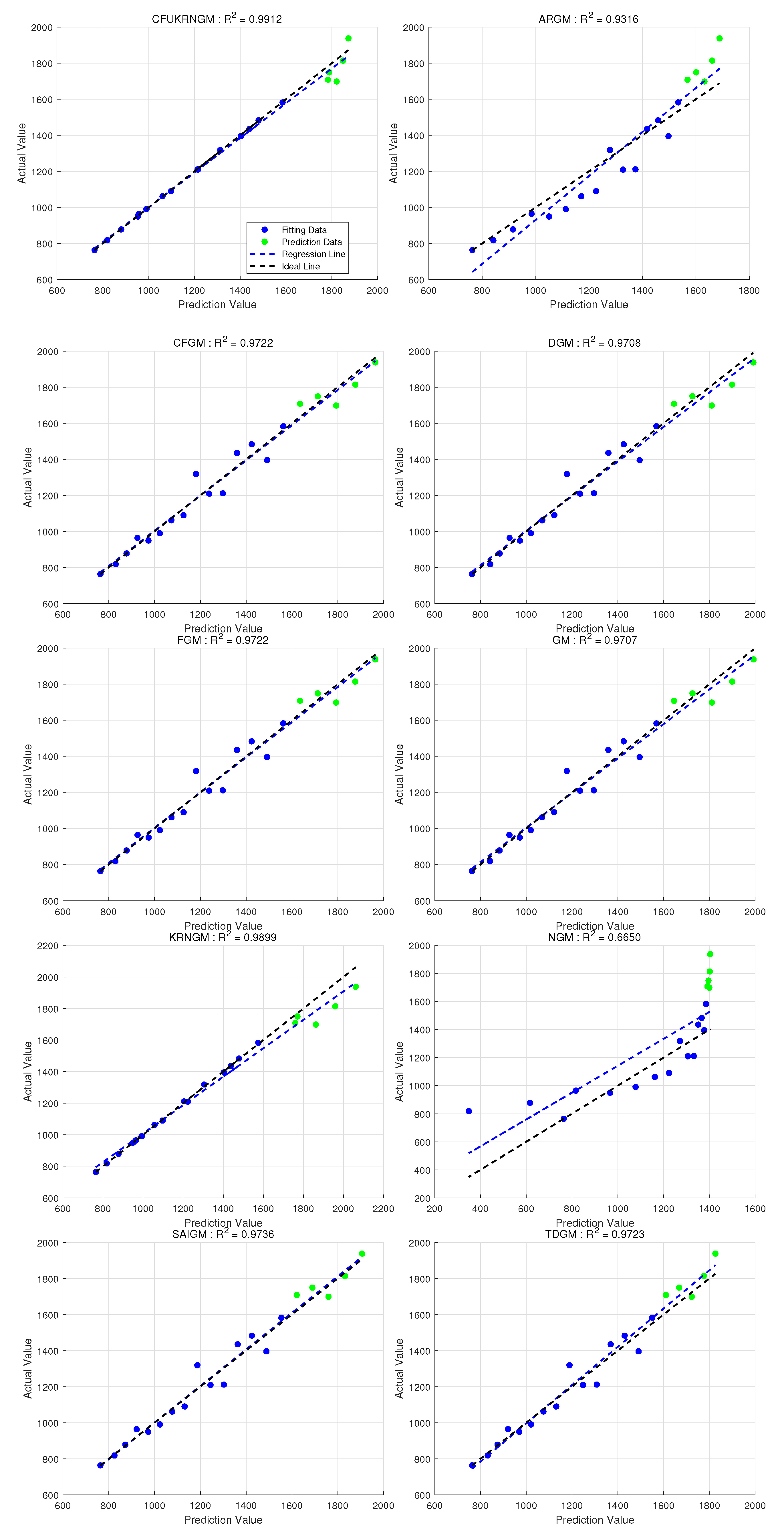
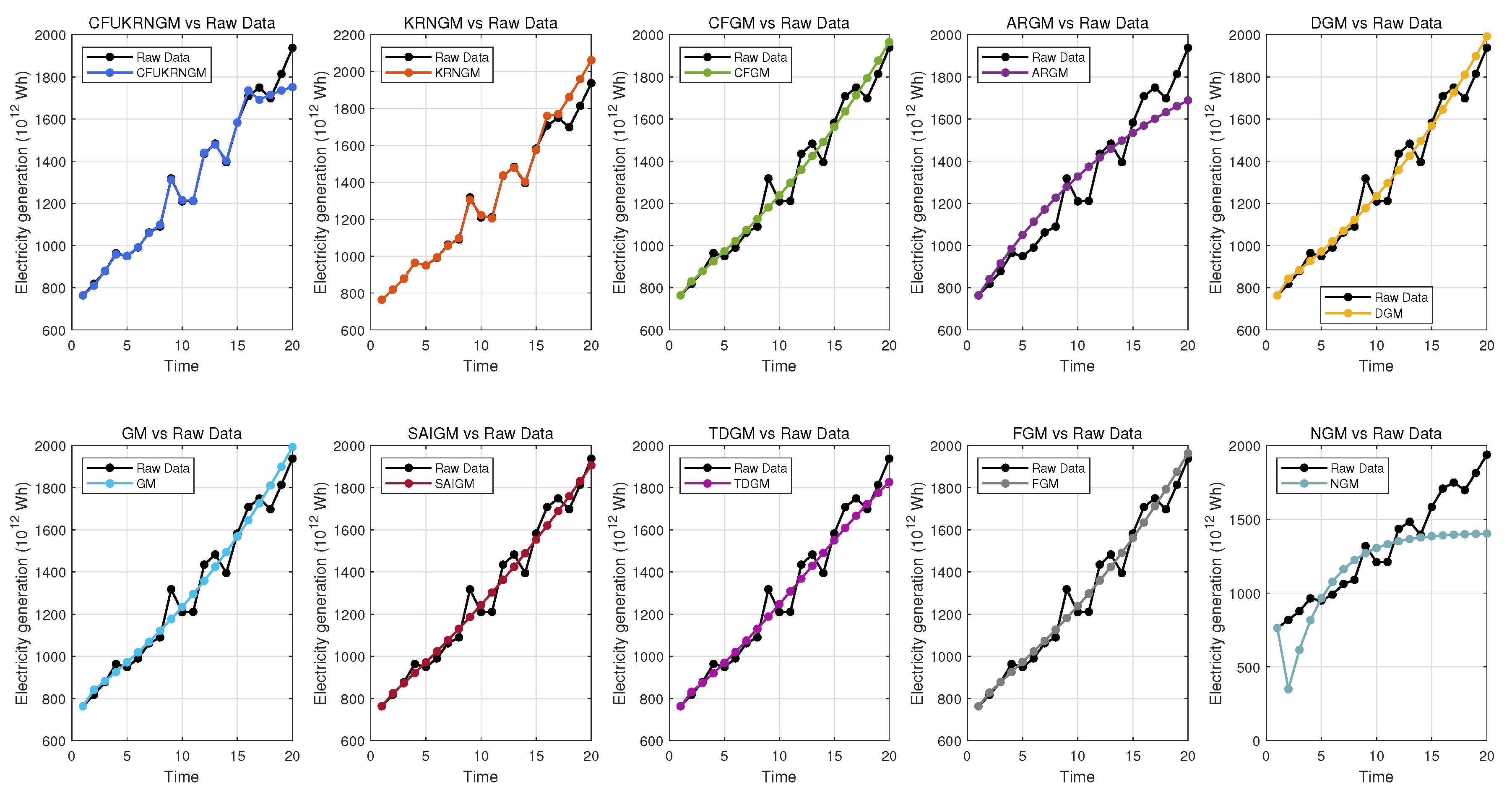
Figure 8 offers an exhaustive comparison of predictive accuracy across all ten models, distinctly demonstrating their individual fitting and forecasting capabilities. The visual comparisons indicate that the CFUKRNGM model’s predictions show an extraordinary level of alignment with the actual data points, as its associated linear regression line closely approximates the ideal reference line. This demonstrates that the CFUKRNGM model accurately reflects the fundamental dynamics and trends of the examined dataset. Thus, through both qualitative visual assessment and quantitative accuracy metrics, the CFUKRNGM model demonstrates the highest reliability and precision in this validation context. Moreover,The anticipated values produced by several grey models, in conjunction with the actual observed data, are depicted in Figure 9.

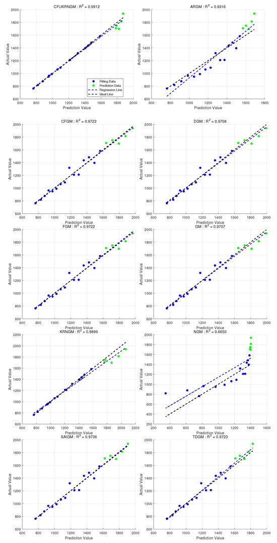
Figure 8. The regression performance of ten grey models in Case 4. $R^2$ represents the coefficient of determination between the raw data and the predicted values of the models (Overall).

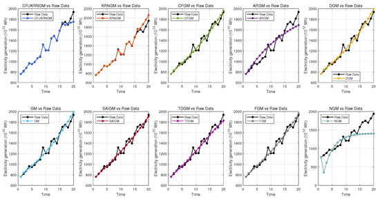
Figure 9. The performance of 10 grey models’ predictions in Case 4.

Table 14 delineates the calculated evaluation metrics for each grey model in this instance. Table 14 demonstrates that the CFUKRNGM model surpasses the others in both fitting historical data and attaining superior predictive accuracy for future data. The CFUKRNGM model exhibits superior performance in both fitting and prediction.

Table 14. The computed evaluation metrics for the prediction results of 10 grey models in Case 4.

Metrics	CFUKRNGM	ARGM	CFGM	DGM	FGM	GM	KRNGM	NGM	SAIGM	TDGM
Fitting RMSE (↓)	5.8836	87.1415	58.0112	58.5286	58.0764	58.5268	6.6559	169.7289	57.8895	57.8325
MAE (↓)	4.7493	70.9890	44.2124	43.9447	43.9046	43.7341	4.9861	126.4018	45.0248	45.1177
NRMSE (↓)	0.5146	7.6214	5.0737	5.1189	5.0794	5.1188	0.5821	14.8445	5.0630	5.0580
MAPE (↓)	0.3895	6.3110	3.5592	3.5779	3.5350	3.5551	0.3957	12.2434	3.6338	3.6539
RMSPE (↓)	0.4744	7.8017	4.5080	4.5499	4.5069	4.5448	0.5253	18.5457	4.5192	4.5315
MSE (↓)	34.6167	7593.6389	3365.2959	3425.5957	3372.8670	3425.3854	44.3007	28807.9108	3351.1989	3344.5959
IA (↑)	0.9994	0.8762	0.9451	0.9441	0.9450	0.9441	0.9993	0.5302	0.9453	0.9455
U1 (↓)	0.0025	0.0365	0.0248	0.0250	0.0248	0.0250	0.0028	0.0737	0.0248	0.0247
U2 (↓)	0.0050	0.0745	0.0496	0.0500	0.0496	0.0500	0.0057	0.1451	0.0495	0.0494
Prediction RMSE (↓)	43.9885	161.7951	60.5482	60.5482	63.4389	74.0770	115.3784	392.2584	57.1716	78.6640
MAE (↓)	39.0028	150.9159	54.9020	54.9020	58.5168	67.7324	101.2688	382.9760	51.6771	70.9901
NRMSE (↓)	14.4429	45.9183	41.5274	42.1727	41.6295	42.2044	39.3578	59.1307	34.3863	19.1493
MAPE (↓)	12.9037	46.3896	41.8662	42.5365	41.9723	42.5695	39.5093	59.9959	34.2980	16.2495
RMSPE (↓)	15.5456	48.9127	44.2576	44.9317	44.3648	44.9644	42.2001	62.4097	36.6595	19.9406
MSE (↓)	298.4790	3017.0218	2467.6132	2544.8987	2479.7622	2548.7300	2216.5021	5003.0382	1691.9107	524.7003
IA (↑)	−0.9758	−18.9711	−15.3343	−15.8459	−15.4147	−15.8712	−13.6721	−32.1174	−10.1995	−2.4732
U1 (↓)	0.0685	0.1872	0.1724	0.1746	0.1727	0.1747	0.1650	0.2285	0.1471	0.0910
U2 (↓)	0.1437	0.4568	0.4131	0.4195	0.4141	0.4198	0.3915	0.5882	0.3421	0.1905

6. Conclusions

In this work, a CFUKRNGM model was proposed to address the limitations of traditional grey models in handling complex nonlinear time series. By integrating CFA into the grey modeling process, the method extracts richer long-memory information from the data. Furthermore, a kernel function satisfying Mercer’s condition was introduced into the nonhomogeneous grey model framework, effectively embedding nonlinearity into the model and eliminating the bias term present in the original KRNGM, thus resulting in an unbiased modeling formulation. The parameter estimation for CFUKRNGM is achieved by solving only a single linear equation of reduced order (lower than that of the standard KRNGM), which simplifies the computational procedure. In addition, the key hyperparameters are automatically tuned using a Bayesian optimization algorithm. These innovations yield a model that preserves the efficiency of grey system models for small-sample forecasting while substantially enhancing their capacity to capture complex, nonlinear patterns in the data.

From a practical application perspective, the CFUKRNGM model has demonstrated strong predictive performance across various energy-related datasets, such as oil production, carbon dioxide emissions, and electricity generation. This not only validates the methodological advancement of the model but also highlights its broad real-world applicability. The model is capable of accurately forecasting energy production trends even with limited sample data, thereby providing quantitative support for energy scheduling, resource planning, and policy formulation. For instance, in oilfield production forecasting, accurately predicting output trends over a future time horizon can help enterprises optimize production plans and reduce resource waste. In the context of carbon emission prediction, the model’s outputs can inform the development of more scientifically grounded emission reduction strategies and energy transition policies. The results demonstrate that the removal of the bias factor and the incorporation of a nonlinear kernel function enhance the CFUKRNGM model’s alignment with the dynamic characteristics of complex data, therefore minimizing prediction errors and effectively mitigating overfitting across diverse settings. Nonetheless, it is important to acknowledge that the model’s effectiveness may still be limited by specific conditions. Excessive noise in the dataset, inadequate training samples, or the use of kernel functions ill-suited to the structural properties of a certain domain may result in diminished predictive accuracy. Furthermore, in situations characterized by significant non-stationarity or sudden alterations in data, the model may find it challenging to reliably identify underlying trends, which potentially leads to discrepancies in predictions. The limits of these models will be essential to our future research endeavors.

In summary, this work presents a unified and efficient grey modeling approach that bridges fractional order techniques with kernel regularization to overcome the linearity and bias limitations of previous models. The CFUKRNGM expands the methodological toolbox of grey system theory, offering a more flexible and accurate framework for time series forecasting under uncertainty. The results suggest that combining advanced mathematical tools (such as conformable fractional operators) with machine learning ideas (such as kernel methods and automatic hyperparameter tuning) can make grey models much better at modeling. Such an approach is not only effective for the cases examined in this study but also holds promise for a wide range of applications involving complex, nonlinear, and small-sample data. Future research can build upon the CFUKRNGM framework to explore other kernel functions or fractional operators and apply this model to diverse domains (e.g., energy consumption, economic indicators, or engineering systems), further extending the reach of grey system modeling in capturing real-world complexities.

References

- Lu, C.; Li, S.; Lu, Z. Building energy prediction using artificial neural networks: A literature survey. Energy Build. 2022, 262, 111718. [Google Scholar] [CrossRef]
- Wang, Z.; Wang, Y.; Zeng, R.; Srinivasan, R.S.; Ahrentzen, S. Random Forest based hourly building energy prediction. Energy Build. 2018, 171, 11–25. [Google Scholar] [CrossRef]
- Fan, C.; Sun, Y.; Zhao, Y.; Song, M.; Wang, J. Deep learning-based feature engineering methods for improved building energy prediction. Appl. Energy 2019, 240, 35–45. [Google Scholar] [CrossRef]
- Cammarano, A.; Petrioli, C.; Spenza, D. Pro-Energy: A novel energy prediction model for solar and wind energy-harvesting wireless sensor networks. In Proceedings of the 2012 IEEE 9th International Conference on Mobile Ad-Hoc and Sensor Systems (MASS 2012), Las Vegas, NV, USA, 8–11 October 2012; pp. 75–83. [Google Scholar]
- He, X.; Wang, Y.; Zhang, Y.; Ma, X.; Wu, W.; Zhang, L. A novel structure adaptive new information priority discrete grey prediction model and its application in renewable energy generation forecasting. Appl. Energy 2022, 325, 119854. [Google Scholar] [CrossRef]
- Feng, S.; Ma, Y.; Song, Z.; Ying, J. Forecasting the energy consumption of China by the grey prediction model. Energy Sources Part Econ. Planning Policy 2012, 7, 376–389. [Google Scholar] [CrossRef]
- Tsai, S.B. Using grey models for forecasting China’s growth trends in renewable energy consumption. Clean Technol. Environ. Policy 2016, 18, 563–571. [Google Scholar] [CrossRef]
- Duan, H.; Pang, X. A multivariate grey prediction model based on energy logistic equation and its application in energy prediction in China. Energy 2021, 229, 120716. [Google Scholar] [CrossRef]
- Ju-Long, D. Control problems of grey systems. Syst. Control Lett. 1982, 1, 288–294. [Google Scholar] [CrossRef]
- Julong, D. Essential Topics on Grey System: Theory and Application. In A Report on the Project of National Science Foundation of China; China Ocean Press: Beijing, China, 1988. [Google Scholar]
- Mao, M.; Chirwa, E.C. Application of grey model GM (1, 1) to vehicle fatality risk estimation. Technol. Forecast. Soc. Change 2006, 73, 588–605. [Google Scholar] [CrossRef]
- Wang, Y.; He, X.; Zhou, Y.; Luo, Y.; Tang, Y.; Narayanan, G. A novel structure adaptive grey seasonal model with data reorganization and its application in solar photovoltaic power generation prediction. Energy 2024, 302, 131833. [Google Scholar] [CrossRef]
- Li, X.; Li, N.; Ding, S.; Cao, Y.; Li, Y. A novel data-driven seasonal multivariable grey model for seasonal time series forecasting. Inf. Sci. 2023, 642, 119165. [Google Scholar] [CrossRef]
- Zhou, W.; Wu, X.; Ding, S.; Ji, X.; Pan, W. Predictions and mitigation strategies of PM2. 5 concentration in the Yangtze River Delta of China based on a novel nonlinear seasonal grey model. Environ. Pollut. 2021, 276, 116614. [Google Scholar] [CrossRef] [PubMed]
- Zhou, W.; Wu, X.; Ding, S.; Cheng, Y. Predictive analysis of the air quality indicators in the Yangtze River Delta in China: An application of a novel seasonal grey model. Sci. Total Environ. 2020, 748, 141428. [Google Scholar] [CrossRef] [PubMed]
- Wu, L.; Liu, S.; Yao, L.; Yan, S.; Liu, D. Grey system model with the fractional order accumulation. Commun. Nonlinear Sci. Numer. Simul. 2013, 18, 1775–1785. [Google Scholar] [CrossRef]
- Wu, L.; Liu, S.; Chen, D.; Yao, L.; Cui, W. Using gray model with fractional order accumulation to predict gas emission. Nat. Hazards 2014, 71, 2231–2236. [Google Scholar] [CrossRef]
- Wang, Y.; Chi, P.; Nie, R.; Ma, X.; Wu, W.; Guo, B. Self-adaptive discrete grey model based on a novel fractional order reverse accumulation sequence and its application in forecasting clean energy power generation in China. Energy 2022, 253, 124093. [Google Scholar] [CrossRef]
- Wensong, J.; Zhongyu, W.; Mourelatos, Z.P. Application of Nonequidistant Fractional-Order Accumulation Model on Trajectory Prediction of Space Manipulator. IEEE/ASME Trans. Mechatronics 2016, 21, 1420–1427. [Google Scholar] [CrossRef]
- Zhang, J.; Qin, Y.; Zhang, X.; Che, G.; Sun, X.; Duo, H. Application of non-equidistant GM (1, 1) model based on the fractional-order accumulation in building settlement monitoring. J. Intell. Fuzzy Syst. 2022, 42, 1559–1573. [Google Scholar] [CrossRef]
- Gao, M.; Mao, S.; Yan, X.; Wen, J. Estimation of Chinese CO2 Emission Based on A Discrete Fractional Accumulation Grey Model. J. Grey Syst. 2015, 27, 114–130. [Google Scholar]
- Ma, X.; Wu, W.; Zeng, B.; Wang, Y.; Wu, X. The conformable fractional grey system model. ISA transactions 2020, 96, 255–271. [Google Scholar] [CrossRef]
- Duan, H.; Lei, G.R.; Shao, K. Forecasting Crude Oil Consumption in China Using a Grey Prediction Model with an Optimal Fractional-Order Accumulating Operator. Complexity 2018, 2018, 3869619. [Google Scholar] [CrossRef]
- Chen, L.; Liu, Z.; Ma, N. Time-Delayed Polynomial Grey System Model with the Fractional Order Accumulation. Math. Probl. Eng. 2018, 2018, 3640625. [Google Scholar] [CrossRef]
- Wu, L.; Gao, X.; Xiao, Y.; Yang, Y.; Chen, X. Using a novel multi-variable grey model to forecast the electricity consumption of Shandong Province in China. Energy 2018, 157, 327–335. [Google Scholar] [CrossRef]
- Cai, M. Non-homogeneous Grey Model NGM (1, 1) with initial value modification and its application. In Proceedings of the 2010 2nd International Conference on Industrial and Information Systems, Dalian, China, 10–11 July 2010; Volume 1, pp. 102–104. [Google Scholar]
- Jiang, J.; Zhang, Y.; Liu, C.; Xie, W. An improved nonhomogeneous discrete grey model and its application. Math. Probl. Eng. 2020, 2020, 4638296. [Google Scholar] [CrossRef]
- Wu, W.; Ma, X.; Zeng, B.; Zhang, P. A Conformable Fractional Non-homogeneous Grey Forecasting Model with Adjustable Parameters CFNGMA (1, 1, k, c) and its Application. J. Grey Syst. 2024, 36, 1–12. [Google Scholar]
- Ma, X.; Hu, Y.s.; Liu, Z.b. A novel kernel regularized nonhomogeneous grey model and its applications. Commun. Nonlinear Sci. Numer. Simul. 2017, 48, 51–62. [Google Scholar] [CrossRef]
- Vapnik, V. Statistical Learning Theory; John Wiley & Sons Google Schola: Hoboken, NJ, USA, 1998; Volume 2, pp. 831–842. [Google Scholar]
- Hofmann, T.; Schölkopf, B.; Smola, A.J. Kernel methods in machine learning. Ann. Stat. 2008, 36, 1171–1220. [Google Scholar] [CrossRef]
- Camastra, F.; Verri, A. A novel kernel method for clustering. IEEE Trans. Pattern Anal. Mach. Intell. 2005, 27, 801–805. [Google Scholar] [CrossRef]
- Blanchard, G.; Bousquet, O.; Zwald, L. Statistical properties of kernel principal component analysis. Mach. Learn. 2007, 66, 259–294. [Google Scholar] [CrossRef]
- Suykens, J.A.; Vandewalle, J. Chaos control using least-squares support vector machines. Int. J. Circuit Theory Appl. 1999, 27, 605–615. [Google Scholar] [CrossRef]
- Wang, H.; Fu, G.; Cai, Y.; Wang, S. Multiple feature fusion based image classification using a non-biased multi-scale kernel machine. In Proceedings of the 2015 12th International Conference on Fuzzy Systems and Knowledge Discovery (FSKD), Zhangjiajie, China, 15–17 August 2015; pp. 700–704. [Google Scholar]
- Wang, S.; Tang, L.; Yu, L. SD-LSSVR-based decomposition-and-ensemble methodology with application to hydropower consumption forecasting. In Proceedings of the 2011 Fourth International Joint Conference on Computational Sciences and Optimization, Kunming and Lijiang City, China, 15–19 April 2011; pp. 603–607. [Google Scholar]
- Juyal, A.; Sharma, S. A Study of landslide susceptibility mapping using machine learning approach. In Proceedings of the 2021 Third International Conference on Intelligent Communication Technologies and Virtual Mobile Networks (ICICV), Tirunelveli, India, 4–6 February 2021; pp. 1523–1528. [Google Scholar]
- Wang, H.Q.; Sun, F.C.; Cai, Y.N.; Ding, L.G.; Chen, N. An unbiased LSSVM model for classification and regression. Soft Comput. 2010, 14, 171–180. [Google Scholar] [CrossRef]
- Jeon, M.; Kim, D.; Lee, W.; Kang, M.; Lee, J. A conservative approach for unbiased learning on unknown biases. In Proceedings of the IEEE/CVF Conference on Computer Vision and Pattern Recognition, New Orleans, LA, USA, 18–24 June 2022; pp. 16752–16760. [Google Scholar]
- de Mello, C.E.R. Active Learning: An Unbiased Approach. Ph.D. Thesis, Ecole Centrale Paris. Universidade federal do Rio de Janeiro, Paris, France, 2013. [Google Scholar]
- Syarif, I.; Prugel-Bennett, A.; Wills, G. SVM parameter optimization using grid search and genetic algorithm to improve classification performance. TELKOMNIKA Telecommun. Comput. Electron. Control 2016, 14, 1502–1509. [Google Scholar] [CrossRef]
- Bergstra, J.; Bengio, Y. Random search for hyper-parameter optimization. J. Mach. Learn. Res. 2012, 13, 281–305. [Google Scholar]
- Holland, J.H. Genetic algorithms. Sci. Am. 1992, 267, 66–73. [Google Scholar] [CrossRef]
- Kennedy, J.; Eberhart, R. Particle swarm optimization. In Proceedings of the ICNN’95-International Conference on Neural Networks, Perth, WA, Australia, 27 November–1 December 1995; Volume 4, pp. 1942–1948. [Google Scholar]
- Bertsimas, D.; Tsitsiklis, J. Simulated annealing. Stat. Sci. 1993, 8, 10–15. [Google Scholar] [CrossRef]
- Brochu, E.; Cora, V.M.; De Freitas, N. A tutorial on Bayesian optimization of expensive cost functions, with application to active user modeling and hierarchical reinforcement learning. arXiv 2010, arXiv:1012.2599. [Google Scholar]
- Mao, S.; Gao, M.; Xiao, X.; Zhu, M. A novel fractional grey system model and its application. Appl. Math. Model. 2016, 40, 5063–5076. [Google Scholar] [CrossRef]
- Xie, N.m.; Liu, S.f. Discrete grey forecasting model and its optimization. Appl. Math. Model. 2009, 33, 1173–1186. [Google Scholar] [CrossRef]
- Zeng, B.; Meng, W.; Tong, M. A self-adaptive intelligence grey predictive model with alterable structure and its application. Eng. Appl. Artif. Intell. 2016, 50, 236–244. [Google Scholar] [CrossRef]
- Ma, X.; Mei, X.; Wu, W.; Wu, X.; Zeng, B. A novel fractional time delayed grey model with Grey Wolf Optimizer and its applications in forecasting the natural gas and coal consumption in Chongqing China. Energy 2019, 178, 487–507. [Google Scholar] [CrossRef]
- Shaikh, F.; Ji, Q.; Shaikh, P.H.; Mirjat, N.H.; Uqaili, M.A. Forecasting China’s natural gas demand based on optimised nonlinear grey models. Energy 2017, 140, 941–951. [Google Scholar] [CrossRef]
- Wu, L.; Liu, S.; Chen, H.; Zhang, N. Using a novel grey system model to forecast natural gas consumption in China. Math. Probl. Eng. 2015, 2015, 686501. [Google Scholar] [CrossRef]
Disclaimer/Publisher’s Note: The statements, opinions and data contained in all publications are solely those of the individual author(s) and contributor(s) and not of MDPI and/or the editor(s). MDPI and/or the editor(s) disclaim responsibility for any injury to people or property resulting from any ideas, methods, instructions or products referred to in the content. |
© 2025 by the authors. Licensee MDPI, Basel, Switzerland. This article is an open access article distributed under the terms and conditions of the Creative Commons Attribution (CC BY) license (https://creativecommons.org/licenses/by/4.0/).