Abstract
Fraud in financial services—especially account opening fraud—poses major operational and reputational risks. Static rules struggle to adapt to evolving tactics, missing novel patterns and generating excessive false positives. Machine learning promises adaptive detection, but deployment faces severe class imbalance: in the NeurIPS 2022 BAF Base benchmark used here, fraud prevalence is 1.10%. Standard metrics (accuracy, f1_weighted) can look strong while doing little for the minority class. We compare Logistic Regression, SVM (RBF), Random Forest, LightGBM, and a GRU model on N = 1,000,000 accounts under a unified preprocessing pipeline. All models are trained to minimize their loss function, while configurations are selected on a stratified development set using validation-weighted F1-score f1_weighted. For the four classical models, class weighting in the loss (class_weight ) is treated as a hyperparameter and tuned. Similarly, the GRU is trained with a fixed class-weighted CrossEntropy loss that up-weights fraud cases. This ensures that both model families leverage weighted training objectives, while their final hyperparameters are consistently selected by the f1_weighted metric. Despite similar AUCs and aligned feature importance across families, the classical models converge to high-precision, low-recall solutions (1–6% fraud recall), whereas the GRU recovers 78% recall at 5% precision (AUC ). Under extreme imbalance, objective choice and operating point matter at least as much as architecture.
1. Introduction
Fraud in the financial services sector is a persistent and evolving threat, extending far beyond transaction-level scams. A particularly costly and growing danger is bank account opening fraud, where criminals use stolen or synthetic identities to establish new accounts [1]. These accounts then serve as conduits for money laundering, unauthorized credit access, and other financial crimes, costing institutions billions annually and posing significant operational and reputational risks [2]. These challenges are not unique to banking; the insurance industry faces analogous problems in claims fraud and identity-related schemes, which present the same data-driven challenges [3,4,5].
Historically, the first line of defense was traditional detection frameworks built on static, hard-coded rules (e.g., flagging mismatched addresses). The core challenge of these systems is their rigidity. As fraud tactics evolve, these static rules fail to adapt, leading to a dual failure: they miss novel fraudulent patterns while simultaneously overwhelming investigators with a high volume of false positives. The velocity of modern digital finance renders these manual or static systems infeasible, creating an urgent need for automated, adaptive solutions [6].
To overcome these limitations, machine learning (ML) has been widely adopted for its ability to learn subtle, complex patterns from heterogeneous data [7]. These models are now critical components of modern FinTech platforms, often deployed on cloud infrastructure to provide the low-latency predictions essential for real-time decisions. However, applying ML in this domain introduces its own formidable challenge: severe class imbalance [8]. In the dataset for this study, fraudulent applications constitute only 1.10% of all cases. This imbalance creates a paradox: models trained to optimize standard metrics (like accuracy or weighted-F1) are incentivized to predict the majority (non-fraud) class, creating a misleading illusion of performance while failing to detect the very events they were built to find [9].
The application of machine learning to financial fraud is well-documented, with extensive surveys highlighting the persistent challenge of class imbalance and rare event detection [10,11]. These comprehensive reviews emphasize a critical pitfall in fraud analytics: the reliance on accuracy-focused evaluation metrics, which can mask poor performance on the minority class. To combat this, the literature has proposed various remediation strategies, ranging from data-level techniques to algorithm-level approaches such as cost-sensitive learning and anomaly detection [12]. However, while these individual methods are well-established, there is often ambiguity regarding the comparative impact of the model architecture versus the optimization objective in extremely imbalanced settings (<1% prevalence). This study builds upon this literature by isolating these factors; rather than proposing a novel complex architecture, we provide a controlled evaluation demonstrating that the choice of objective function outweighs the choice of model family.
This paper provides a rigorous empirical comparison of classical and deep learning approaches on a large-scale, public benchmark for bank account fraud detection [13]. We systematically evaluate a suite of models: Logistic Regression (LR) [14], Support Vector Machine (SVM) [15], Random Forest (RF) [16], LightGBM (LGBM) [17], and a custom Gated Recurrent Unit (GRU) network [18]. We specifically investigate how these models behave under a common hyperparameter-tuning rule while retaining the default training objectives of their respective Python 3.12.12 implementations. Concretely, all models share the same preprocessing pipeline and are tuned on a stratified development set using the validation-weighted F1-score (f1_weighted) as the selection metric, while each model optimises the default loss provided by its underlying Python function, with class weighting enabled when selected during hyperparameter search.
Our results demonstrate two key findings. First, we confirm that all classical models optimized for standard metrics show limited efficacy, identifying almost no fraudulent cases (1–6% recall). Second, we show that the GRU model, trained with a class-weighted loss function, successfully overcomes this challenge, identifying 78% of all fraud. However, this success exposes the central, practical challenge of this domain: a severe precision–recall trade-off [19]. The high recall is achieved at the cost of extremely low precision (5%), creating a significant operational burden of false positives.
1.1. Motivation and Research Questions
We frame the study around three research questions (RQs) that the industry faces under extreme imbalance:
- RQ1: How do classical models (LR, SVM, RF, LGBM) behave when tuned and selected using f1_weighted on a 1.10% prevalence dataset, and what failure modes emerge for the minority class?
- RQ2: To what extent can a class-weighted objective (here, with a GRU) recover minority-class recall, and what precision (false-positive workload) trade-offs does this entail?
- RQ3: Do model families converge on the same high-signal features, implying that objective choice—not signal scarcity—drives minority-class performance gaps?
1.2. Contributions
This paper makes four contributions aligned with those questions:
- A controlled, apples-to-apples comparison on the 1M-example BAF “Base” benchmark with a unified preprocessing pipeline across classical models and a GRU architecture.
- An explicit demonstration of the objective-induced failure: using f1_weighted as the selection criterion yields negligible fraud recall despite apparently strong aggregate scores.
- Evidence that class-weighted training substantially increases recall (to 78%) while quantifying the implied review burden (low precision); we report simple workload proxies (e.g., FPs per TP) alongside standard metrics.
- A cross-family feature importance concordance showing that all models surface the same core signals (e.g., name_email_similarity, velocity_24h), supporting the claim that objective choice—not feature discovery—explains the gap.
1.3. Terminology and Evaluation Framing
Throughout, we use operational cost to denote the human-review workload implied by false positives at the chosen operating threshold. While ROC-AUC remains informative for ranking, at 1.10% prevalence we emphasize precision–recall behavior and report weighted-F1 only to reflect legacy selection practices that can mislead in this setting.
1.4. Scope and Limitations
The focus is account opening fraud on the BAF synthetic benchmark; we do not model post-opening transactional streams, cost-sensitive training beyond class weighting, or production controls (e.g., case management, feedback loops). As the dataset is synthetic, external validity may vary by institution and geography; nevertheless, the imbalance-driven phenomena we document are generic to credit, banking, and insurance onboarding contexts.
Finally, through a comparative feature importance analysis, we show that all models—both the failing classical ones and the successful GRU—demonstrate a high degree of consensus on the most predictive features, such as name_email_similarity and velocity_24h. This provides the critical insight that the failure of the classical models was not one of feature identification, but one of objective. This paper’s contribution is a rigorous analysis of this trade-off, demonstrating how, in an imbalanced domain, the problem shifts from one of detection (recall) to one of operational cost (precision).
2. Methods
This section presents the methodological framework developed to systematically evaluate the effectiveness of classical and deep learning models for a highly imbalanced financial fraud detection task [6]. We begin by describing the dataset and the robust preprocessing pipeline constructed to handle mixed numerical and categorical data types. Next, we outline the architectures and optimization procedures for traditional machine learning (LR, SVM, RF, LGBM) and an advanced recurrent neural model (GRU), including the specific hyperparameter tuning strategies employed. We then define the quantitative evaluation metrics, with a focus on statistical validation via bootstrapping, which is essential for imbalanced classification. Finally, we detail the model-specific and model-agnostic techniques used to compute and compare feature importance, a critical step for model interpretability.
2.1. Data Preprocessing and Preparation
This study utilizes the Bank Account Fraud (BAF) dataset, a large-scale, privacy-preserving benchmark for tabular fraud detection released at NeurIPS 2022 [13]. We use the “Base” variant, which contains approximately one million (N = 1,000,000) synthetic bank account applications generated from a real-world, anonymized source. Each record is described by a range of features and includes a binary label, fraud_bool (1: fraud; 0: non-fraud), to indicate if the application was fraudulent.
It is important to clarify the provenance of this data. The BAF dataset is synthetic, generated using a tabular Generative Adversarial Network (GAN) trained on real-world transaction data to preserve privacy while maintaining statistical fidelity. As a synthetic dataset, it avoids the privacy constraints of real banking data but relies on the assumption that the GAN successfully captured the complex interactions of real-world fraud. It specifically models “synthetic identity fraud,” where criminals combine real (e.g., social security numbers) and fake (e.g., names/emails) information to create a new, fictitious identity.
A defining characteristic of this dataset is its severe class imbalance. Fraudulent applications constitute only 1.10% of the total records (11,029 fraud instances vs. 988,971 non-fraud instances). This severe imbalance is the central methodological challenge that informs our strategies for model training, hyperparameter tuning, and evaluation [20].
To ensure consistent and reproducible feature engineering, a comprehensive preprocessing pipeline was constructed using scikit-learn’s ColumnTransformer [21]. The raw dataset contains 32 columns. After excluding the target label (fraud_bool), 31 potential features remain. From these, we explicitly removed two uninformative columns, source and month, resulting in exactly 29 input features used for modeling. These comprised 16 numerical features (e.g., income, velocity_6h, customer_age) and 13 categorical features (e.g., payment_type, employment_status, device_os). The pipeline applied distinct transformations to each data type:
- Numerical Feature Pipeline: Numerical features were processed with a two-step sequence. First, missing values were imputed using the median value of the respective column. Second, all numerical features were standardized using StandardScaler, transforming them to have a mean of 0 and a standard deviation of 1.
- Categorical Feature Pipeline: Categorical features were similarly processed. First, missing values were imputed with a constant string placeholder ("__missing__"). Second, the features were transformed using OneHotEncoder, which creates a sparse binary vector for each unique category.
This preprocessor object was fit only
The original training data, X_train, consisted of 800,000 records and 31 features. For the deep learning approach (GRU), the 29 selected raw features were used directly as an input sequence (). For the classical models, after applying the preprocessor, which uses 16 numerical features and 13 categorical features, the categorical variables were expanded, meaning the final, transformed data matrix had 59 features. This resulted from the 16 numerical features being scaled and the 13 categorical features being one-hot encoded into 43 distinct columns. The final test set was similarly transformed from (200,000, 31) to (200,000, 59).
2.2. Experimental Setup
To facilitate rigorous model development and evaluation, the dataset was partitioned into several distinct sets:
- Training and Test Split: The full dataset (N = 1,000,000) was divided into a primary training set (80%, or 800,000 records) and a final, held-out test set (20%, or 200,000 records). This split was stratified by the fraud_bool label to ensure the 1.10% positive class ratio was precisely maintained in both partitions.
- Hyperparameter Tuning Set: As grid-searching on 800,000 records is computationally prohibitive, a smaller development set (N = 10,000) was created by subsampling from the training set, again using stratification. This smaller, balanced set was used for the GridSearchCV process for all classical machine learning models.
- Deep Learning Split: For the GRU model, the 800,000-record training set was further subdivided into a new training partition (80%, or 640,000 records) and a validation partition (20%, or 160,000 records). This split was used for the randomized hyperparameter search and for early stopping during model training.
Reproducibility and Environment
All experiments were executed in Google Colab using the standard CPU/GPU runtimes available at the time of study. Because Colab environments are ephemeral and hardware/library versions may vary across sessions, we fixed global random seeds across Python/numpy/scikit-learn/PyTorch and kept all preprocessing fit strictly on the training split. Hyperparameter searches were bounded by a per model family wall-clock budget with graceful early termination, returning the incumbent best configuration. These practices allowed re-runs in Colab to match our reported performance within expected stochastic variation, without relying on a fixed machine image.
2.3. Model Architectures
We implemented and evaluated a suite of four classical machine learning models and one deep learning model, each selected to represent a different class of algorithmic approach to this classification problem.
2.3.1. Classical Machine Learning Models
Logistic Regression (LR)
Logistic regression serves as a high-performing, interpretable linear baseline [14]. Given the preprocessed feature vector , the probability of the positive class () is modeled as
where is the coefficient vector, b is the bias, and is the sigmoid function. Parameters are estimated by minimizing the regularized binary CrossEntropy loss:
where is the predicted probability for sample i and is the regularization strength.
Support Vector Machine (SVM)
The Support Vector Machine (SVM) is a non-linear classifier that finds an optimal separating hyperplane by maximizing the margin between classes [15,22]. For a given dataset where , the SVM solves the following primal optimization problem:
where C is a regularization hyperparameter that controls the trade-off between maximizing the margin and minimizing classification error, are slack variables that permit misclassifications, and is a kernel function that maps the input data into a higher-dimensional feature space. In this study, we evaluated the Radial Basis Function (RBF) kernel, defined as
where is a kernel hyperparameter.
Random Forest (RF)
Random Forest is an ensemble-based algorithm that constructs a multitude of decision trees at training time [23] and outputs the class that is the mode of the classes’ output by individual trees [16,24]. By introducing randomness through two mechanisms, it reduces the high variance and overfitting propensity of individual decision trees.
- Bagging (Bootstrap Aggregating): Each tree in the forest is trained on a different bootstrapped sample (a random sample with replacement) from the training data.
- Feature Randomness: At each node in a tree, a split is determined by searching over only a random subset of m features (where , the total number of features).
For a forest of B trees , the final prediction for a binary class is determined by a majority vote:
where is the indicator function.
Light Gradient Boosting Machine (LightGBM)
LightGBM is a high-performance framework based on the principles of gradient boosting [25] that builds an ensemble of decision trees sequentially [17]. Unlike Random Forest, which builds independent trees, boosting builds trees in an additive, stage-wise manner, where each new tree is fit to correct the errors (residuals) of the previous model :
where is the learning rate. The model is optimized by minimizing a loss function using gradient descent. At each step m, the new tree is fit to the negative gradient (pseudo-residual) of the loss:
LightGBM introduces two key innovations for efficiency: (1) Gradient-based One-Side Sampling (GOSS), which prioritizes training on data points with larger gradients (i.e., those that are poorly classified); (2) Exclusive Feature Bundling (EFB), which groups sparse, mutually exclusive features to reduce dimensionality.
2.3.2. Deep Learning Model: Gated Recurrent Unit (GRU) Model
To capture complex, non-linear feature interactions, we designed a custom deep learning model (GRUSentimentModel) that treats the tabular data as an ordered sequence. The core of this model is the Gated Recurrent Unit (GRU) [18], an advanced recurrent neural network (RNN) cell designed to mitigate the vanishing gradient problem.
Unlike the classical models which utilize sparse one-hot encoded vectors, the GRU processes the raw feature values directly. From the 31 available raw features in the dataset, we excluded two columns (source and month) to prevent noise, resulting in an input sequence length of . The ordering of features in the sequence is deterministic, following the column index of the raw dataframe (e.g., income at index 0, name_email_similarity at index 1). This ensures that the model learns temporal-like dependencies between specific attribute pairs across the dataset.
Given an input sequence of feature embeddings , the GRU computes a hidden state at each step t using two gates: an update gate and a reset gate .
The reset gate determines how to combine the new input with the previous memory, and the update gate controls how much of the previous memory to keep. A candidate hidden state is then computed:
Finally, the output hidden state is an interpolation between the previous state and the candidate state , controlled by the update gate :
where is the sigmoid function, tanh is the hyperbolic tangent, ⊙ is element-wise multiplication, and are learnable parameters. The final hidden state is passed through a Dropout and a final fully-connected layer for classification.
To explicitly address the severe class imbalance during optimization, we implemented a class-weighted training pipeline. The full training procedure, including the calculation of inverse-frequency weights and their application to the CrossEntropy loss, is detailed in Algorithm 1.
| Algorithm 1 Class-Weighted GRU Training Pipeline |
Input: Dataset X (), Binary Labels y, Positive Class Count Hyperparameters: Epochs E, Batch Size B, Learning Rate Output: Optimized Model Parameters // 1. Calculate Inverse-Frequency Class Weights Define Loss Function // 2. Training Loop Initialize GRU parameters (Embedding , Hidden H, Output Linear) for epoch to E do for batch in do
{Shape: } {Apply Class-Weighted Loss} end for end for Return |
2.4. Model Training and Hyperparameter Tuning
All models were optimized using strategies appropriate for their architecture and the severe class imbalance.
- Classical Models (LR, SVM, RF, LGBM): These models were tuned using an exhaustive GridSearchCV with 3-fold cross-validation, performed on the stratified development set. The primary scoring metric used for hyperparameter selection was the validation-weighted F1-score (f1_weighted).
- GRU Model: The deep learning model was tuned using a randomized search () on the 640k/160k train/validation split. The search optimized key hyperparameters including embedding_dim (150–250), hidden_dim (256–768), and learning_rate (–). The best configuration was likewise selected using the validation weighted F1-score (f1_weighted) on the development set, consistent with the classical models.
- Imbalance Handling: This was the primary focus of training.
- For classical models, the class_weight=’balanced’ parameter was included in the grid search, which automatically adjusts weights inversely proportional to class frequencies.
- For the GRU model, this was implemented by calculating class weights on the training set and passing them to the nn.CrossEntropyLoss(weight=...) function. This penalizes misclassifications of the minority (fraud) class more heavily.
To facilitate complete reproduction of these results and allow other researchers to build upon this work, the full source code—including the preprocessing pipeline, class-weight implementation, and model training scripts—are available on the first author’s GitHub (https://github.com/wn-nwN/fraud-detection-project-Nov2025, accessed on 1 December 2025).
2.5. Evaluation Metrics
Given the severe class imbalance, accuracy is a misleading metric [20]. Our evaluation focused on a suite of metrics that provide a nuanced view of model performance on both the minority and majority classes [19]. For a binary classification problem, we define true positives (TPs), false positives (FPs), and false negatives (FNs).
Precision measures the proportion of positive (fraud) predictions that were correct. High precision is critical to minimizing operational costs from false alarms.
Recall (or True Positive Rate) measures the proportion of actual fraud cases that the model successfully identifies. High recall is critical for minimizing risk and preventing fraudulent transactions.
The F1-score is the harmonic mean of precision and recall, providing a single score that balances this trade-off [19]. We report the weighted F1-score as a primary metric, which accounts for the class imbalance.
For all point-estimate metrics (precision, recall, F1), we utilize the standard classification threshold of . While we acknowledge that operational thresholds in fraud detection are typically tuned to specific cost constraints (as discussed in Section 4), utilizing a fixed, neutral threshold of 0.5 allows for a consistent, “ceteris paribus” comparison of the intrinsic probability distributions generated by the different architectures.
Furthermore, we assess the model’s ability to distinguish between classes using the Receiver Operating Characteristic (ROC) curve and its corresponding Area Under the Curve (AUC).
The AUC represents the probability that the model will rank a randomly chosen positive sample higher than a randomly chosen negative sample.
To assess the stability of our point-estimate metrics, we implemented a bootstrapping procedure ( iterations) to compute the 95% Confidence Intervals (CIs) for both the weighted F1-Score and the AUC on the test set.
2.6. Feature Importance Analysis
To ensure model interpretability and understand the key drivers of fraud, we employed a combination of model-specific and model-agnostic techniques.
- Coefficient-Based (LR): For the Logistic Regression model, the absolute values of the fitted coef_ corresponding to each feature were used as direct measures of importance.
- Tree-Based (RF, LGBM): For the ensemble tree models, the native feature_importances_ attribute was used. This score is typically based on Gini impurity reduction (RF) or gain (LGBM) aggregated across all trees in the ensemble.
- Permutation Importance (SVM, GRU): For the non-linear ‘rbf’ SVM and the ‘black-box’ GRU model, we used permutation feature importance. This model-agnostic technique measures the decrease in the model’s F1-score when the values of a single feature are randomly shuffled. This procedure was executed for 6–10 repeats on a 3000-record subsample for computational efficiency. For the GRU, this was performed on the original features (e.g., income) before the embedding stage to maintain interpretability.
3. Results
This section presents the empirical results of the machine learning and deep learning models, evaluated on the held-out test set (N = 200,000). The analysis is presented in two parts. First, we examine the performance of the classical models as optimized by the GridSearchCV process, which used f1_weighted as its primary scoring metric. Second, we analyze the performance of models specifically re-trained using the class_weight=’balanced’ technique to address the severe class imbalance.
3.1. Hyperparameter Optimization and Tuning Cost
Table 1 summarizes the best settings identified by cross-validated search (see Section 2) and the wall-clock time required to complete tuning for each model. The classical baselines converged quickly (5.4–46.6 s): the SVM favored an RBF kernel with and , while Logistic Regression selected regularization with the lbfgs solver. For tree/boosting models, the optimizer preferred using class weighting (class_weight=balanced); Random Forest settled on a moderate depth () with 200 trees, and LightGBM retained a compact configuration (, , 100 estimators).

Table 1.
Optimal hyperparameters and tuning times for all models.
In contrast, the GRU required substantially more compute to tune (4118.1 s), with the selected setting using an embedding dimension , a large hidden size , a low learning rate (), and eight epochs. This was ∼763× slower than Logistic Regression, ∼189× slower than SVM, and ∼88–144× slower than the tree/boosting models, reflecting the higher search cost of neural architectures relative to classical methods.
Overall, tuning time spans nearly three orders of magnitude across models, which has practical implications for iteration speed and deployment. When compute or turnaround time is constrained, the linear, SVM, and tree/boosting families provide more favorable tuning efficiency than the GRU, while still allowing targeted adjustments (e.g., class weighting for imbalanced data). All timings were obtained under the same environment; details are provided in Methods.
3.2. Analysis of Model Performance
The results reveal two distinct patterns of model behavior, highlighting the critical impact of class imbalance and the choice of loss function.
3.2.1. Performance Limitations of Classical Models
As shown in Table 2, the four classical machine learning models (SVM, LR, RF, LGBM) all appear to perform exceptionally well, with weighted precision, recall, and F1-scores at or above 0.98. However, these metrics are highly misleading. Because the models were tuned using validation-weighted F1-score (f1_weighted) as the hyperparameter selection metric, a quantity dominated by the 98.9% majority (non-fraud) class, they learned to achieve a high score by simply predicting “non-fraud” for nearly every case.
Table 2.
Overall performance of all models on the test set.
It is crucial to note that for Random Forest and LightGBM, the hyperparameter search explicitly selected class_weight=‘balanced’ (see Table 1). Despite this mechanism—which increases penalties for minority class errors—the models still converged on a high-precision/low-recall solution. This underscores a critical finding: simply enabling a “balanced” mode in standard libraries is often insufficient to overcome the inertia of the majority class if the global validation metric (here, f1_weighted) does not explicitly prioritize recall.
This limited effectiveness to solve the practical problem is confirmed in Table 3. The Class 1 recall is minimal: the SVM and LR models detect only 1% of fraudulent transactions, while the RF and LGBM models detect only 6%. Despite achieving high overall AUCs, these models are insufficient for deployment as they fail to identify the target class.
Table 3.
Minority fraud class (Class 1) performance of all models.
3.2.2. The Precision–Recall Trade-Off in the GRU Model
In stark contrast, the Gated Recurrent Unit (GRU) model, which was trained with a class-weighted loss function, successfully learned to identify the minority class. This is immediately visible in Table 2, where its weighted recall (0.83) is much lower than the other models, indicating it is not just predicting the majority class.
Table 3 shows the true result: the GRU model successfully identified 78% of all fraudulent transactions (recall = 0.78), a substantial improvement over the classical models. Furthermore, its AUC of 0.8800 was the highest of all models, confirming its superior ability to distinguish between the two classes.
However, this success in detection reveals the central challenge of this dataset. The high recall was achieved at the cost of extremely low precision. With a Class 1 precision of 0.05, the model generates approximately 19 false positives for every one true positive it finds. This demonstrates a classic precision–recall trade-off, where the model is effective at finding fraud but creates a significant operational burden in doing so.
3.3. Operational Impact and Workload Analysis
To contextualize operations, we report the implied review load at the chosen threshold. With Class 1 precision , the ratio of false positives to true positives is
i.e., roughly 19 alerts to review for each correctly detected fraud.
To quantify this for a business context, consider a financial institution processing N = 1,000,000 applications with the dataset’s 1.1% fraud prevalence (11,000 fraud cases).
- Detection Volume: With 78% recall, the model correctly identifies 8580 fraud cases.
- False Alert Volume: At 5% precision, these 8580 cases represent only 1/20th of the total flag volume. The model generates approximately 163,000 false positives.
- Total Review Queue: The total volume of alerts requiring human review would be ≈171,600.
- Staffing Implication: Assuming a fraud analyst can review 50 cases per day, this model configuration would require approximately 13–14 full-time analysts working for a full year (260 working days) just to clear the backlog for one million applications.
This calculation explicitly demonstrates the resource cost mentioned by the reviewers: high recall comes with a substantial labor overhead.
3.4. Feature Importance and Model Interpretation
To understand the predictive logic of the models, we computed feature importances for all five architectures (Figure 1, Figure 2, Figure 3, Figure 4 and Figure 5). For LR, RF, and LGBM, we used their native model-based importances (coefficient magnitude or Gini/gain). For the non-linear SVM and the GRU, we used permutation importance based on the drop in the F1-score.
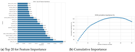
Figure 1.
SVM feature importance (permutation).
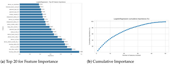
Figure 2.
Logistic Regression feature importance (absolute coefficients).
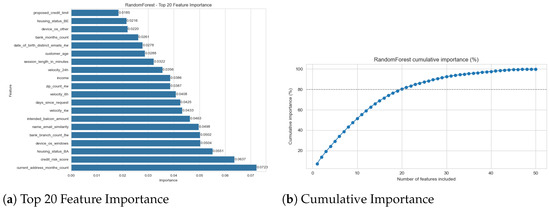
Figure 3.
Random Forest Feature Importance (Gini).
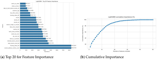
Figure 4.
LightGBM feature importance (gain).
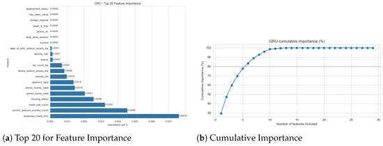
Figure 5.
GRU feature importance (permutation).
The most significant finding is the high degree of consensus across all models. Despite their vastly different architectures and performance, all models identified the same core set of features as the most predictive. The feature name_email_similarity was the undisputed top predictor for all five models, often by a significant margin (see Figure 1a and Figure 2a, etc.). To clarify, this feature represents a normalized string distance metric (ranging from 0 to 1) between the applicant’s provided name and their email user handle. A low score indicates a mismatch (e.g., “John Doe” using “hacker123@email.com”), which is a primary indicator of synthetic identity fraud where criminals use burner email addresses with stolen personal details.
This consensus extends to other top-tier features. The high importance of velocity_24h and velocity_6h is similarly logical; these features track the count of applications associated with the same device or IP address within a 6 h or 24 h sliding window. High values are a proxy for automated “bot” attacks or “bust-out” fraud schemes where criminals attempt to open multiple accounts in rapid succession. The income feature is also a key differentiator, likely because fraudulent applications may use anomalously high or low values that deviate from the patterns of legitimate applicants. The consistency of these findings provides strong evidence that all models, regardless of their success, are identifying the correct, fundamental signals in the data.
This analysis provides a critical insight when combined with the performance results from Section 3. The performance gap of the classical models (LR, SVM, RF, LGBM) was not a failure of feature identification; they correctly identified the same predictive features as the successful GRU model. Their failure was one of objective. This is, in itself, an important finding: the feature importance plots for the classical models effectively show us the hallmarks of a non-fraudulent application.
Summary
Taken together with the performance analysis, these attributions indicate that the classical models did not fail to discover informative signals; rather, tuning for f1_weighted as the selection criterion under 1.10% prevalence biased them toward confident non-fraud predictions, whereas the class-weighted GRU leveraged the same signals to recover minority-class recall at the expected cost in precision.
4. Discussion
The empirical results of this study provide a clear and nuanced narrative regarding the application of machine learning to a severely imbalanced fraud detection task. Our findings are discussed in three parts: an interpretation of the primary precision–recall trade-off, the practical implications for real-world systems, and the limitations of this study.
4.1. Interpretation of Key Findings
The central finding of this paper is not simply that one model outperformed another, but that the choice of optimization objective is profoundly more important than the choice of model architecture.
The four classical models (SVM, LR, RF, LGBM) were not inherently “bad.” On the contrary, their high AUC scores (see Table 2) and their feature importance plots (Figure 2, Figure 3 and Figure 4) prove they were highly effective at one task: identifying the correct features. The feature importance analysis shows a clear consensus: all models, including the GRU, agreed that features like name_email_similarity and velocity_24h were the most predictive. The failure of the classical models was one of objective. Tuned using f1_weighted as the validation selection metric, a quantity dominated by the 98.9% majority class, the models learned it was statistically “safer” to ignore the rare fraud signals and become expert detectors of non-fraud. Their resulting 1–6% fraud recall is a direct and predictable outcome of this objective mismatch. This confirms the warnings found in earlier surveys [10] regarding the dangers of accuracy-driven optimization, but extends those findings by quantifying exactly how much ‘architecture’ matters when the objective is misaligned.
The GRU model, in contrast, was a statistical success precisely because its objective (a class-weighted loss) was aligned with the problem. It was explicitly instructed to find the rare class, and it did, achieving a 78% recall. This confirms that the predictive signals for fraud do exist in the data and that a deep learning architecture can effectively leverage them. However, this statistical success immediately exposed the true challenge of this domain: a severe precision–recall trade-off [19].
4.2. Practical Implications: An Operational Bottleneck
The GRU model’s performance—78% recall at 5% precision—perfectly illustrates the difference between a statistical solution and a practical one. While identifying 78% of fraud is a significant achievement, the 5% precision is operationally untenable in many business contexts. This metric implies that for every 100 applications flagged for manual review, 95 are false positives. This would overwhelm a human investigation team and likely be more costly than the fraud it prevents.
This necessitates a shift from purely performance-based evaluation to economic cost considerations, as demonstrated by Vanini et al. [12]. In their work, integrating economic costs into the model selection process led to substantial loss reductions by optimizing for low false-positive rates. Similarly, our findings suggest that a bank cannot simply deploy the “best AUC” model; they must determine an “optimal” threshold based on their specific risk appetite and regulatory tolerance.
For instance, a regulated institution facing heavy fines for money laundering (AML) violations might tolerate the high operational cost of the 5% precision model to ensure maximum recall. Conversely, a FinTech platform focused on frictionless user experience might prefer a stricter threshold to reduce customer friction. In a hypothetical scenario used for illustration, such an institution might accept a lower recall of 50% in exchange for a precision of 20%. This alignment of model thresholds with institutional strategy resonates with broader finance research on risk behavior, where the salience of specific risks drives decision-making [26]. Ultimately, the “right” model is not defined by the F1-score, but by the institution’s capacity to absorb the cost of intervention versus the cost of fraud losses.
The practical value of this GRU model, therefore, is not as a final decision-maker. Instead, it should be viewed as an exceptionally effective triage and filtering tool. It successfully reduced the problem from 1 million “unknown” applications to a much smaller, high-risk pool, which can then be fed into a more specialized (or costly) second-stage analysis. This suggests a hybrid approach, where the high-recall/low-precision model serves as the first-pass filter for a system designed to manage, rather than eliminate, the operational cost of false positives.
4.3. Limitations and Future Work
This study’s findings, while clear, are bounded by several methodological choices that open avenues for future research.
- Choice of Imbalance Technique: We focused exclusively on one technique: class-weighted loss. This is a powerful method, but it is not the only one. Future work should compare our GRU’s performance against other strategies, such as algorithm-level approaches (e.g., Focal Loss [8]) or data-level approaches (e.g., SMOTE oversampling or undersampling the majority class).
- Deep Learning Architectures: The GRU, a recurrent model, was used to process tabular data as a sequence. While effective, it is not a traditional architecture for this data type. A valuable next step would be to benchmark this model against transformers designed specifically for tabular data, such as a TabTransformer, to see if attention-based mechanisms can better model the feature interactions.
- Generalizability and Fraud Prevalence: Our analysis relies on the BAF dataset with a fixed 1.1% fraud prevalence. While this is representative of many onboarding scenarios, findings may differ in domains with moderately higher prevalence (e.g., credit card fraud at 5–10%) or different feature distributions. Future studies should simulate varying prevalence rates (e.g., by subsampling negatives) to determine the “break-even” point where classical models might recover performance.
- Alternative Strategies (Ensembles): We treated models as competitors, but in practice, they can be collaborators. A promising avenue for future work is to explore ensemble or two-stage architectures. For example, the high-recall GRU could serve as a “nominator” to flag potential fraud, while a high-precision Random Forest could serve as a “validator” to filter out false positives. Such hybrid approaches could potentially optimize the precision–recall trade-off better than any single model.
- Threshold Tuning: Our results report metrics at the default 0.5 classification threshold. Given the severe precision–recall trade-off, this is not the optimal threshold for deployment. A critical next step, which we recommend for any practical application, is to analyze the full precision–recall curve (which is more informative than the ROC curve in imbalanced settings [9,20]). By “moving the threshold,” an organization could select a different operating point, for example, hypothetically accepting a lower recall of 50% in exchange for a more manageable precision of 20%.
- Analysis of False Positives: The 5% precision of the GRU model is not merely a performance deficit; it is a source of data. A qualitative analysis of the false positives—the legitimate cases that “look” fraudulent to the model—could reveal new insights, identify feature engineering opportunities, or highlight biases in the dataset [27].
4.4. Concluding Remarks
Taken together, our results show that in extremely imbalanced onboarding settings the decisive levers are what we optimize and where we operate, rather than model family per se. On the BAF benchmark, standard f1_weighted selection produced classical baselines with superficially strong aggregate scores yet negligible fraud recall, whereas a class-weighted GRU recovered minority detection (78% recall) at the expected cost in precision (5%). For practice, this reframes fraud modeling as a joint objective–threshold design problem: align the training objective with minority-class capture and set the operating point to the review budget and risk tolerance. For research, it motivates reporting precision–recall behavior and simple workload proxies (e.g., FPs per TP) alongside aggregate metrics to make operational trade-offs explicit. This clarity—of objective, operating point, and reporting—provides a principled path from statistical performance to deployable value.
Author Contributions
Conceptualization, S.X.; Methodology, W.S. and Q.S.; Software, W.S. and Q.S.; Validation, Q.M.; Investigation, Y.G.; Resources, T.Q.; Writing—original draft, S.X.; Writing—review and editing, S.X. All authors have read and agreed to the published version of the manuscript.
Funding
This research received no external funding.
Data Availability Statement
The original data presented in the study are openly available in Kaggle at https://www.kaggle.com/datasets/sgpjesus/bank-account-fraud-dataset-neurips-2022 (accessed on 11 November 2025).
Conflicts of Interest
The authors declare no conflicts of interest.
References
- Aite-Novarica Group. Synthetic Identity Fraud: The Elephant in the Room; Technical Report; Aite-Novarica Group: Boston, MA, USA, 2021. [Google Scholar]
- Hernandez Aros, L.; Bustamante Molano, L.X.; Gutierrez-Portela, F.; Moreno Hernandez, J.J.; Rodríguez Barrero, M.S. Financial fraud detection through the application of machine learning techniques: A literature review. Humanit. Soc. Sci. Commun. 2024, 11, 1130. [Google Scholar] [CrossRef]
- Aslam, F.; Hunjra, A.I.; Ftiti, Z.; Louhichi, W.; Shams, T. Insurance fraud detection: Evidence from artificial intelligence and machine learning. Res. Int. Bus. Financ. 2022, 62, 101744. [Google Scholar] [CrossRef]
- Liu, Y.; Shen, X.; Zhang, Y.; Wang, Z.; Tian, Y.; Dai, J.; Cao, Y. A systematic review of machine learning approaches for detecting deceptive activities on social media: Methods, challenges, and biases. Int. J. Data Sci. Anal. 2025, 20, 6157–6182. [Google Scholar] [CrossRef]
- Tian, Y.; Xu, S.; Cao, Y.; Wang, Z.; Wei, Z. An empirical comparison of machine learning and deep learning models for automated fake news detection. Mathematics 2025, 13, 2086. [Google Scholar] [CrossRef]
- Xu, S.; Cao, Y.; Wang, Z.; Tian, Y. Fraud detection in online transactions: Toward hybrid supervised–unsupervised learning pipelines. In Proceedings of the 6th International Conference on Electronic Communication and Artificial Intelligence (ICECAI 2025), Chengdu, China, 20–22 June 2025. [Google Scholar]
- Baisholan, N.; Dietz, J.E.; Gnatyuk, S.; Turdalyuly, M.; Matson, E.T.; Baisholanova, K. A Systematic Review of Machine Learning in Credit Card Fraud Detection Under Original Class Imbalance. Computers 2025, 14, 437. [Google Scholar] [CrossRef]
- Boabang, F.; Goussiatiner, S.A. An Enhanced Focal Loss Function to Mitigate Class Imbalance in Auto Insurance Fraud Detection. arXiv 2025, arXiv:2508.02283. [Google Scholar] [CrossRef]
- Saito, T.; Rehmsmeier, M. The precision–recall plot is more informative than the ROC plot when evaluating binary classifiers on imbalanced datasets. PLoS ONE 2015, 10, e0118432. [Google Scholar] [CrossRef] [PubMed]
- Ali, A.; Shukor, A.R.; Omar, S.H.; Abdu, S. Financial fraud detection based on machine learning: A systematic literature review. Appl. Sci. 2022, 12, 9637. [Google Scholar] [CrossRef]
- West, J.; Bhattacharya, M. Intelligent financial fraud detection: A comprehensive review. Comput. Secur. 2016, 57, 47–66. [Google Scholar] [CrossRef]
- Vanini, P.; Rossi, S.; Zvizdić, E.; Domenig, T. Online payment fraud: From anomaly detection to risk management. Financ. Innov. 2023, 9, 66. [Google Scholar] [CrossRef]
- Jesus, S.; Pombal, J.; Alves, D.; Cruz, A.; Saleiro, P.; Ribeiro, R.P.; Gama, J.; Bizarro, P. Turning the Tables: Biased, Imbalanced, Dynamic Tabular Datasets for ML Evaluation. In Advances in Neural Information Processing Systems; Curran Associates, Inc.: Red Hook, NY, USA, 2022. [Google Scholar]
- Hosmer, D.W.; Lemeshow, S.; Sturdivant, R.X. Applied Logistic Regression, 3rd ed.; John Wiley & Sons, Inc.: New York, NY, USA, 2013. [Google Scholar]
- Van Craen, A.; Breyer, M.; Pflüger, D. PLSSVM—Parallel Least Squares Support Vector Machine. Softw. Impacts 2022, 14, 100343. [Google Scholar] [CrossRef]
- Manzali, Y.; Elfar, M. Random Forest Pruning Techniques: A Recent Review. Oper. Res. Forum 2023, 4, 43. [Google Scholar] [CrossRef]
- Ke, G.; Meng, Q.; Finley, T.; Wang, T.; Chen, W.; Ma, W.; Ye, Q.; Liu, T.Y. LightGBM: A highly efficient gradient boosting decision tree. In Proceedings of the 31st International Conference on Neural Information Processing Systems (NeurIPS), Long Beach, CA, USA, 4–9 December 2017; pp. 3149–3157. [Google Scholar]
- Cho, K.; van Merriënboer, B.; Gulcehre, C.; Bahdanau, D.; Bougares, F.; Schwenk, H.; Bengio, Y. Learning Phrase Representations Using RNN Encoder–Decoder for Statistical Machine Translation. In Proceedings of the 2014 Conference on Empirical Methods in Natural Language Processing (EMNLP), Doha, Qatar, 25–29 October 2014; pp. 1724–1734. [Google Scholar]
- Powers, D.M.W. Evaluation: From precision, recall and F-measure to ROC, informedness, markedness and correlation. J. Mach. Learn. Technol. 2011, 2, 37–63. [Google Scholar]
- Davis, J.; Goadrich, M. The relationship between Precision-Recall and ROC curves. In Proceedings of the 23rd International Conference on Machine Learning (ICML), Pittsburgh, PA, USA, 25–29 June 2006; pp. 233–240. [Google Scholar]
- Pedregosa, F.; Varoquaux, G.; Gramfort, A.; Michel, V.; Thirion, B.; Grisel, O.; Blondel, M.; Prettenhofer, P.; Weiss, R.; Dubourg, V.; et al. Scikit-learn: Machine Learning in Python. J. Mach. Learn. Res. 2011, 12, 2825–2830. [Google Scholar]
- Cortes, C.; Vapnik, V. Support-Vector Networks. Mach. Learn. 1995, 20, 273–297. [Google Scholar] [CrossRef]
- Breiman, L.; Friedman, J.H.; Olshen, R.A.; Stone, C.J. Classification and Regression Trees; Wadsworth & Brooks/Cole Advanced Books & Software: Monterey, CA, USA, 1984. [Google Scholar]
- Breiman, L. Random forests. Mach. Learn. 2001, 45, 5–32. [Google Scholar] [CrossRef]
- Friedman, J.H. Greedy function approximation: A gradient boosting machine. Ann. Stat. 2001, 29, 1189–1232. [Google Scholar] [CrossRef]
- Mugerman, Y.; Steinberg, N.; Wiener, Z. The exclamation mark of Cain: Risk attitude and mutual fund flows. J. Bank. Financ. 2022, 134, 106332. [Google Scholar] [CrossRef]
- Cao, Y.; Dai, J.; Wang, Z.; Zhang, Y.; Shen, X.; Liu, Y.; Tian, Y. Machine learning approaches for depression detection on social media: A systematic review of biases and methodological challenges. J. Behav. Data Sci. 2025, 5, 67–102. [Google Scholar] [CrossRef]
Disclaimer/Publisher’s Note: The statements, opinions and data contained in all publications are solely those of the individual author(s) and contributor(s) and not of MDPI and/or the editor(s). MDPI and/or the editor(s) disclaim responsibility for any injury to people or property resulting from any ideas, methods, instructions or products referred to in the content. |
© 2025 by the authors. Licensee MDPI, Basel, Switzerland. This article is an open access article distributed under the terms and conditions of the Creative Commons Attribution (CC BY) license (https://creativecommons.org/licenses/by/4.0/).