Adaptive Measurement Noise Covariance Estimation for GNSS/INS Tightly Coupled Integration Using a Linear-Attention Transformer with Residual Sparse Denoising and Channel Attentions

Abstract

Tightly coupled GNSS/INS is a widely adopted architecture for UAVs and ground vehicles. In this study, a Kalman-filter-based fusion framework integrates inertial data with satellite observables, including pseudorange and Doppler-derived range rate, to sustain precise navigation when GNSS quality degrades. A key bottleneck is that many pipelines rely on fixed or overly simplified measurement-noise covariance models, which cannot track the nonstationary statistics of real observations. To address this issue, we develop an adaptive covariance estimator built on a Transformer enhanced with three modules: a Linear-Attention layer, a Residual Sparse Denoising Autoencoder (R-SDAE), and a lightweight residual channel-attention block (LRCAM). The estimator predicts the measurement-noise covariance online. R-SDAE distills sparse, outlier-resistant features from noisy ephemeris; LRCAM reweights informative channels via residual gating; and Linear Attention preserves long-range spatiotemporal dependencies while reducing attention cost from O(N²) to O(N). A predictive factor further modulates the covariance for improved efficiency and adaptability. Experimental results on real road-test data show that the proposed method achieves sub-meter positioning accuracy in open-sky conditions and preserves meter-level accuracy with improved robustness under GNSS-degraded urban scenarios, outperforming the compared adaptive-filtering baselines and neural covariance estimators and thereby demonstrating superior positioning accuracy and stability.

1. Introduction

In GNSS/INS integrated navigation, the inertial navigation system (INS) operates autonomously, performing navigation computations without external aids [1]. It delivers a high update rate and strong short-term accuracy [2]; however, its errors grow with time, causing a gradual loss of positioning precision [3]. In contrast, the Global Navigation Satellite System (GNSS) attains high accuracy in open-sky conditions but suffers from degradation or outages in urban canyons, tunnels, and beneath elevated structures [4]. Consequently, combining GNSS with INS has become a principal strategy to exploit their complementary strengths for precise and robust navigation [5]. Among available architectures, the loosely coupled (LC) scheme is straightforward to implement due to its simple structure [6], yet it requires at least four visible satellites to form a position solution, which restricts use under weak or obstructed signals [7]. By comparison, the tightly coupled (TC) scheme directly fuses raw GNSS measurements with INS outputs, sustaining state updates and navigation corrections even when fewer than four satellites are available, thereby offering improved environmental adaptability and robustness [8].

In complex settings, tightly coupled (TC) navigation generally attains higher positioning accuracy. When satellite signals are obstructed, however, the statistics of measurement noise become uncertain and time-varying, and inaccurate modeling of these statistics can trigger filter divergence, observed as fast growth of state errors, leading to drift or even failure [9]. TC architectures typically exploit raw GNSS observables—e.g., pseudorange and pseudorange rate—to calibrate INS errors [10]. Conventional methods often treat the measurement-noise covariance as a fixed prior, a simplification that cannot capture the operational variability of the noise [11]. To cope with this, practical systems commonly adopt adaptive Kalman filtering (AKF) to estimate the observation-noise covariance $R$ online, thereby sustaining solution continuity and positioning accuracy [12]. Moreover, AKF adjusts the filter gain using real-time measurement statistics, preserving stability under unknown or abruptly changing noise conditions and thus providing improved robustness and adaptability.

In recent years, deep learning has advanced rapidly in areas such as computer vision and natural language processing [13]. By means of gradient back-propagation with error feedback, these models uncover hidden structures in data and continually adjust their internal parameters to form effective feature representations. Exploiting the ability of neural networks to capture nonlinear, high-dimensional dependencies, this work embeds a deep-learning-based adaptive noise estimator within the tightly coupled navigation framework. The estimator is trained offline using high-precision reference trajectories and predicts the measurement-noise covariance online during operation, thereby allowing the Kalman filter to adapt to environmental changes.

In conventional practice, inaccurate characterization of noise statistics prevents the system model from faithfully representing the physical process, producing a mismatch between observations and model predictions that can lead to filter divergence [14]. Because noise properties in real deployments are inherently uncertain and time-varying, assuming them to be fixed constants is unrealistic. Consequently, adapting the statistical properties of the measurement-noise covariance to the prevailing environment is more consistent with the dynamics of navigation systems and improves positioning stability and accuracy in challenging operating conditions [15].

To cope with the uncertainty of measurement-noise covariance in GNSS/INS integration, a range of adaptive filtering strategies has been explored across different application settings. Cho and Choi combined a Sigma-Point Kalman Filter (SPKF) with a receding-horizon scheme, using a finite update window to curb initial estimation errors and suppress time-varying biases [16]. Zhang et al. employed the Sage–Husa framework for online estimation of measurement-noise statistics, adapting parameters in real time to accommodate noise variation [17]. Xu et al. proposed a simplified Sage–Husa variant that lowers the computational burden while retaining reliable covariance estimation [18]. Moreover, Ge et al. designed an adaptive Unscented Kalman Filter based on covariance matching, which markedly enhances the robustness and stability of the standard UKF under non-ideal noise conditions [19].

Beyond the above methods, covariance-matching approaches adaptively infer the process- and measurement-noise covariances at each sample by exploiting the innovation or residual covariance. When the adaptive update is driven directly by innovation sequences, large estimation errors may appear, which can degrade navigation accuracy and even induce filter divergence [20]. To cope with uncertainty in noise statistics, Ge et al. proposed a redundant-measurement-driven adaptive estimator for GNSS/INS integration [21]; it forms inter-difference sequences from INS solutions and, together with an MCC-EKF, updates the measurement-noise covariance online, improving robustness. On this basis, Huang et al. [12] developed a Bayesian adaptive Kalman filtering scheme that estimates the process and measurement covariances jointly and online, alleviating the coupling between (Q) and (R) during simultaneous estimation [22]. To further enhance positioning accuracy and robustness, Sun et al. introduced an adaptive method using pseudorange-error prediction with an ensemble learner to model differential sequences and track time-varying measurement-noise covariance, thereby suppressing GNSS observation disturbances [23]. Addressing frequent GNSS errors in urban scenarios, Li et al. built a bagged-regression-tree predictor for pseudorange error and used its outputs to adjust the covariance dynamically, improving the accuracy and stability of tightly coupled GNSS/INS [24]. To strengthen the performance under model uncertainty, Ding et al. proposed a Bayesian-inference-based adaptive UKF that jointly estimates dynamic parameters and measurement-noise statistics, markedly improving filter robustness [25]. For maneuvering-target tracking with time-varying noise, Zhao et al. combined the IMM approach with an adaptive UKF to realize online covariance estimation and robust performance in complex environments [26].

In recent years, given the strong data-modeling capacity of neural networks in vision and language tasks, their integration with Kalman filtering (KF) has been increasingly investigated to boost GNSS/INS positioning accuracy. Vega-Brown et al. proposed Backprop KF, which learns the time-varying patterns of measurement covariance to refine state-error modeling and correct prediction uncertainty during inference [27]. Revach, G. introduced DeepKF, employing neural networks to infer the observation covariance while enforcing positive-definite outputs, thereby improving both estimation accuracy and uncertainty representation [28]. Md Fazle Rabby. developed an RNN-based KF (RNN-KF) that jointly adapts measurement and process noise parameters while capturing system dynamics, reducing reliance on large training corpora [29]. Wu et al. presented a multi-task deep-learning adaptive KF that treats navigation as an interactive environment and optimizes the filter via an observation-error-driven reward, enabling online joint estimation of process and measurement covariances [30]. He et al. further proposed a Bayesian multi-task learning approach that simultaneously estimates both covariances within the KF, markedly enhancing adaptability and robustness in dynamic, non-ideal conditions [31].

We present a Transformer-based framework for predicting measurement-noise covariance that integrates three modules—Residual Sparse Denoising Autoencoder (R-SDAE), Linear Attention, and a Lightweight Residual Channel-Attention Module (LRCAM)—to realize adaptive covariance adjustment. In preprocessing, the R-SDAE first denoises and reconstructs measurement streams (e.g., pseudorange and range rate), suppressing anomalies arising from urban occlusion, multipath, and abrupt disturbances. The Transformer backbone then employs Linear Attention to extract temporal representations, preserving long-range dependency modeling while markedly reducing computational cost. In parallel, LRCAM performs residual-domain channel recalibration in a lightweight manner, which strengthens the characterization of measurement-uncertainty features. The attention-enhanced representations produced by these modules drive the online update of the measurement-noise covariance within the Kalman filter, yielding substantial gains in robustness and positioning accuracy under complex, dynamic conditions. Experiments on real road-test data show that the proposed method outperforms the considered adaptive filtering baselines and the compared neural covariance estimators, including CNN, LSTM, and the standard Transformer, in navigation accuracy and robustness, while maintaining a practical inference cost for the GNSS measurement-update stage.

The remainder of this paper is organized as follows. Section 2 introduces the system model and the proposed method. Section 3 presents the experimental results and performance evaluation. Section 4 discusses the main findings and limitations. Section 5 concludes the paper and outlines future work.

2. System Model and Methodology

In this study, a tightly coupled GNSS/INS integrated navigation system is adopted for its superior performance compared with the loosely coupled architecture. The standard tightly coupled integration framework is illustrated in Figure 1, where the differences between the GNSS pseudorange and pseudorange rate measurements and their corresponding INS-derived predicted measurements are input into the Kalman filter (KF) to estimate the INS errors [32]. These estimated errors are then used to correct the INS outputs, yielding accurate navigation solutions. Unlike the loosely coupled approach, which requires at least four visible satellites for position updates, the tightly coupled system directly utilizes the raw GNSS observations (pseudorange and pseudorange rate) as measurement inputs. This enables the system to maintain a reliable positioning performance even when the number of visible satellites falls below four. Based on this framework, the proposed method further incorporates an adaptive measurement noise covariance estimation module to dynamically adjust the covariance matrix R, thereby enhancing the robustness and accuracy of the navigation filter under complex and time-varying environments.

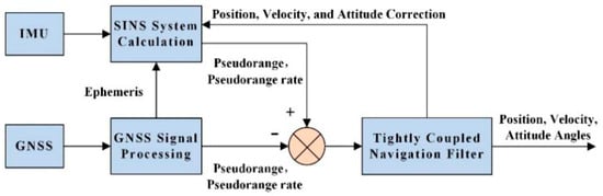
Figure 1. Tightly coupled navigation mode.

2.1. SINS/GNSS Tightly Coupled State Equation

The establishment of the tightly coupled navigation state equation first requires selecting an appropriate state vector. The state vector chosen in this paper is

$$X={\left[\begin{array}{c}\delta {\phi }_x,\delta {\phi }_y,\delta {\phi }_z,\delta V_E,\delta V_N,\delta V_U,\delta L,\delta \lambda ,\delta h,\\ {ϵ}_{bx},{ϵ}_{by},{ϵ}_{bz},{\nabla }_{bx},{\nabla }_{by},{\nabla }_{bz},\delta t,\delta \dot{t}\end{array}\right]}^{\mathrm{\top }}$$

(1)

where $\delta {\phi }_x,\delta {\phi }_y,\delta {\phi }_z$ represent the attitude error angles in the three axes; $\delta V_E,\delta V_N,\delta V_U$ represent the velocity errors in the east, north, and up directions; $\delta L,\delta \lambda ,\delta h$ represent the latitude, longitude, and altitude errors; ${ϵ}_{bx},{ϵ}_{by},{ϵ}_{bz}$ represent the gyro biases along the three axes in the body frame; ${\nabla }_{bx},{\nabla }_{by},{\nabla }_{bz}$ represent the accelerometer biases along the three axes in the body frame; $\delta t$ represents the clock bias equivalent distance; and $\delta \dot{t}$ represents the clock drift rate equivalent distance variation [33].

The tightly coupled state equation is

$$\dot{X}\left(t\right)=F\left(t\right)X\left(t\right)+G\left(t\right)W\left(t\right)$$

(2)

where $F\left(t\right)$ is the state transition matrix, $G\left(t\right)$ is the system noise input matrix, and $W\left(t\right)$ is the system noise matrix. By establishing the attitude error equation, velocity error equation, position error equation, gyroscope error equation, accelerometer error equation, and the GNSS clock bias and clock drift error models, the specific expressions for $F\left(t\right)$ and $G\left(t\right)$ can be derived [34].

The specific expression for the system noise matrix $W\left(t\right)$ is

$$W\left(t\right)={\left[{\omega }_{gx},{\omega }_{gy},{\omega }_{gz},{\omega }_{ax},{\omega }_{ay},{\omega }_{az},{\omega }_{tu},{\omega }_{tru}\right]}^{\mathrm{T}}$$

(3)

where ${\omega }_{gi}\left(i=x,y,z\right)$ represents the white noise of the gyroscopes along the three axes in the body frame, ${\omega }_{ai}\left(i=x,y,z\right)$ represents the white noise of the accelerometers along the three axes in the body frame, and ${\omega }_{tu}$ and ${\omega }_{tru}$ represent the white noise of the clock bias and clock drift, respectively.

2.2. SINS/GNSS Tightly Coupled Measurement Equation

The tightly coupled measurement equation selects the pseudorange difference and pseudorange rate difference as the measurement vector:

$$Z=\left[\begin{array}{c}\delta \rho \\ \delta \dot{\rho }\end{array}\right]=\left[\begin{array}{c}{\rho }_G-{\rho }_{\mathrm{S}\mathrm{I}\mathrm{N}\mathrm{S}}\\ {\dot{\rho }}_G-{\dot{\rho }}_{\mathrm{S}\mathrm{I}\mathrm{N}\mathrm{S}}\end{array}\right]$$

(4)

where ${\rho }_{\mathrm{G}}$ and ${\dot{\rho }}_{\mathrm{G}}$ are the GNSS-measured pseudorange and pseudorange rate, respectively; and ${\rho }_{\mathrm{S}\mathrm{I}\mathrm{N}\mathrm{S}}$ and ${\dot{\rho }}_{\mathrm{S}\mathrm{I}\mathrm{N}\mathrm{S}}$ are the corresponding predicted pseudorange and pseudorange rate computed from the current SINS-derived position and velocity together with the receiver clock bias and clock drift states, respectively.

By establishing the measurement equations for the pseudorange and pseudorange rate, the measurement equation for the SINS/GNSS tightly coupled system can be expressed as:

$$\mathrm{Z}=\left[\begin{array}{l}{H}_{\rho }\left(t\right)\\ H_{\dot{\rho }}\left(t\right)\end{array}\right]X+\left[\begin{array}{l}{V}_{\rho }\left(t\right)\\ V_{\dot{\rho }}\left(t\right)\end{array}\right]$$

(5)

where $H_{\rho }\left(t\right)$ and $H_{\dot{\rho }}\left(t\right)$ are the observation matrices for the pseudorange and pseudorange rate, respectively; and $V_{\rho }\left(t\right)$ and $V_{\dot{\rho }}\left(t\right)$ are the white noise terms for the pseudorange and pseudorange rate, respectively [34].

2.3. EKF-Based Navigation Integration

The outputs of the INS and GNSS subsystems are fused by an Extended Kalman Filter (EKF). The EKF operates recursively, with the time-update (prediction) stage written as [35]:

$$\{\begin{array}{c}{x}_k^{-}={\Phi }_{k,k-1}{x}_{k-1}^{+}\\ P_k^{-}={\Phi }_{k,k-1}{P}_{k-1}^{+}{\Phi }_{k,k-1}^T+Q_{k-1}\end{array}$$

(6)

where $x_{k-1}^{+}$ denotes the estimated state at time k − 1, $P_{k-1}^{+}$ is the corresponding covariance matrix of the estimation error, $x_k^{-}$ and $P_k^{-}$ represent the predicted state and the predicted covariance matrix at time k, respectively, ${\Phi }_{k,k-1}$ is the state transition matrix, and $Q_{k-1}$ represents the process noise covariance matrix.

The measurement update equations are expressed as follows:

$$\{\begin{array}{c}{K}_k=P_k^{-}{H}_k^T{\left(H_k{P}_k^{-}{H}_k^T+R_k\right)}^{-1}\\ x_k^{+}=x_k^{-}+K_k\left(\delta Z_k-H_k{x}_k^{-}\right)\\ P_k^{+}=\left(I-K_k{H}_k\right)P_k^{-}\end{array}$$

(7)

where $\delta Z_k$ represents the measurement innovation vector, $H_k$ denotes the measurement matrix, $K_k$ is the Kalman gain, and $R_k$ represents the measurement noise covariance matrix. In the measurement-update step, the adaptively updated $R_k$ enters the innovation covariance $\dot{S_k}=H_k\dot{P_k^{-}{H}_k^{\mathrm{\top }}}+R_k$, and thus directly affects the Kalman gain and the relative weighting between the predicted state and the incoming GNSS observations. In implementation, $R_k$ is kept non-negative, and the posterior covariance is updated in Joseph form to improve numerical robustness and better preserve symmetry and positive semidefiniteness under finite-precision computation.

2.4. RLL-AKF Framework

This section introduces the overall framework of the RLL-AKF algorithm. The proposed method is built upon a GNSS/INS tightly coupled structure, integrating deep learning modules to achieve adaptive modeling and dynamic adjustment of the measurement noise covariance matrix R. The overall architecture is illustrated in Figure 2. In the data preprocessing stage, a Residual Sparse Denoising Autoencoder (R-SDAE) is employed to reconstruct and denoise raw measurements such as pseudorange and pseudorange rate, effectively suppressing abnormal observations caused by signal blockage, multipath effects, and sudden interference. Subsequently, the backbone network adopts a Transformer architecture enhanced with a Linear Attention mechanism, which efficiently captures long-term temporal dependencies while significantly reducing computational complexity. Finally, a Lightweight Residual Channel Attention Module (LRCAM) is incorporated to further strengthen the local modeling capability for measurement uncertainty. The features extracted from these modules are ultimately used to drive the Kalman filter for adaptive updating of the measurement noise covariance, thereby improving the system’s robustness and navigation accuracy under complex and dynamic environments. The following subsections describe the implementation of each module in detail.

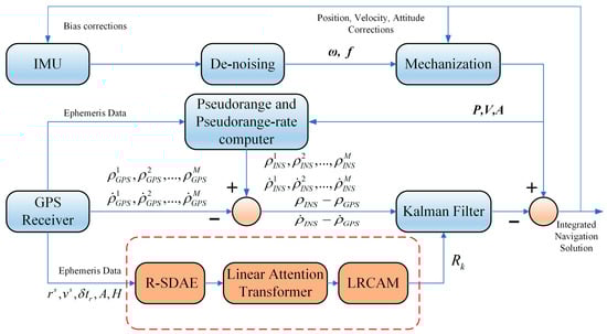
Figure 2. Workflow of the proposed tightly coupled GNSS/INS integration.

2.4.1. Residual Sparse Denoising Autoencoder (R-SDAE)

In complex environments, ephemeris- and observation-derived features are often contaminated by signal blockage, multipath, and transient interference, which degrade the quality of pseudorange and pseudorange rate measurements. To improve feature robustness, an R-SDAE module is introduced as a denoising front end. By combining residual convolution with sparse activation, the module learns stable latent representations from partially corrupted inputs. During training, a DropMask mechanism randomly masks local elements of the input feature matrix to mimic observation loss and local anomalies, while a sparsity regularizer suppresses abnormal activations and improves generalization. As shown in Figure 3, both the encoder and decoder adopt sparse convolution and residual connections rather than fully connected layers, enabling stronger feature extraction and noise suppression [36].

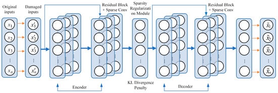
Figure 3. Schematic of the proposed R-SDAE network.

At time step t, the input feature vector is defined as

$$x\left(t\right)=\{r^s\left(t\right),v^s\left(t\right), \Delta t_r\left(t\right),A\left(t\right),H\left(t\right)\}$$

(8)

where $r^s\left(t\right)$ and $v^s\left(t\right)$ denote the satellite position and velocity, respectively; $\Delta t_r\left(t\right)$ represents the receiver clock bias correction term; and $A\left(t\right)$ and $H\left(t\right)$ correspond to the azimuth and elevation angles.

To enhance the model’s robustness against observation noise and missing data under complex environmental conditions, a DropMask operation is applied for random degradation.

$${\mathrm{x}}^{\prime }\left(t\right)=\mathbf{m}\left(t\right)\odot \mathbf{x}\left(t\right),m_{\mathrm{i}}\left(t\right)\sim \mathrm{Bernoulli}\left(1 - p\right)$$

(9)

Here, ⊙ denotes the Hadamard product, and $p\in \left(0, 1\right)$ represents the dropout probability, used to simulate observation loss caused by signal blockage or interruption.

The R-SDAE adopts a residual sparse convolutional encoder–decoder framework, formulated as

$$\mathrm{z}\left(t\right)=E_{\theta }\left(x^{\prime }\left(t\right)\right),\tilde{\mathbf{x}}\left(t\right)={\mathrm{D}}_{\varphi }\left(\mathbf{z}\left(t\right)\right)$$

(10)

where $\mathbf{z}\left(t\right)$ denotes the latent feature representation, and $E_{\theta }$ and $D_{\varphi }$ are the encoding and decoding mapping functions, respectively.

The network is trained to minimize a joint loss function combining the reconstruction error and sparsity constraint:

$$\mathrm{L}={\displaystyle \frac{1}{T}}{\sum }_{t=1}^T{\rho }_{\delta }\left(\mathbf{x}\left(t\right) - \tilde{\mathbf{x}}\left(t\right)\right)+{\lambda }_{\mathrm{KL}}{\sum }_{j=1}^{\mathrm{h}}\mathrm{KL}\left(\rho \parallel {\widehat{\rho }}_j\right)$$

(11)

where ${\rho }_{\delta }\left(\cdot \right)$ is the Huber loss function (δ > 0), and h denotes the hidden unit index.

$${\widehat{\rho }}_j={\displaystyle \frac{1}{T}}{\sum }_{t=1}^T{a}_j\left(t\right),\mathrm{K}\mathrm{L}\left(\rho \parallel {\widehat{\rho }}_j\right)=\rho \ln {\displaystyle \frac{\rho }{{\widehat{\rho }}_j}}+\left(1 - \rho \right)\ln {\displaystyle \frac{1 - \rho }{1 - {\widehat{\rho }}_j}}$$

(12)

Here, ${\widehat{\rho }}_j$ represents the average activation of the j-th hidden neuron, $a_j\left(t\right)$ denotes the activation value of that neuron at time t, and $\rho \in (0, 1)$ is the target sparsity parameter. ${\lambda }_{\mathrm{KL}}$ > 0 is the regularization coefficient.

After completing the unsupervised pre-training process, supervised fine-tuning is performed. The latent features extracted by the encoder are fed into a Transformer with linear attention, which captures long-term temporal dependencies efficiently. Subsequently, the LRCAM module enhances local feature representations through channel recalibration. The dynamically adjusted covariance, generated from these learned features, is then used to adaptively update the measurement noise covariance in the Extended Kalman Filter (EKF) framework. This joint structure effectively optimizes GNSS/INS tightly coupled navigation performance, improving both estimation accuracy and stability.

2.4.2. Adaptive Modeling of Measurement Noise Covariance with a Linear-Attention Transformer

This section presents a Transformer with Linear Attention for adaptive estimation of the measurement-noise covariance in tightly coupled GNSS/INS navigation. The network is coupled with the EKF in an end-to-end differentiable loop and is trained using epochs for which reliable RTK-fixed reference solutions are available. At each epoch, the input sequence is organized per satellite and includes the satellite position, satellite velocity, receiver clock bias, azimuth, and elevation. The network outputs per-satellite noise descriptors for the pseudorange and pseudorange rate, from which the measurement-noise covariance matrix $R_k$ is updated online. These predicted noise descriptors are assembled into the per-epoch covariance matrix $R_k$, which is then used directly in the standard EKF measurement-update step. In this way, the predicted covariance adjusts the observation weighting through the Kalman gain, while the state-transition model and recursive EKF structure remain unchanged.

Compared with the standard scaled dot-product attention, Linear Attention models inter-satellite spatiotemporal correlations with linear complexity, improving scalability for long observation sequences. The predicted covariance is then used in the EKF measurement update, and the position error with respect to the reference trajectory is backpropagated to jointly optimize the network and covariance-generation process. This supervision strategy, however, depends on the availability of reliable RTK-fixed or equivalent high-precision reference trajectories during model development, which may limit its direct applicability in scenarios where such labels cannot be obtained. It should also be noted that RTK-fixed solutions are used here as practical high-precision references rather than error-free ground truth, since they may still contain residual uncertainty caused by satellite geometry, multipath, ambiguity resolution, and synchronization effects. The detailed implementation procedure is summarized in Algorithm 1.

Algorithm 1: Adaptive Estimation of Measurement Noise Covariance (RLL-AKF)

Input: satellite ephemeris/observation features. Output: navigation state (position/velocity/attitude) with updated $R$. 1. Procedure: Model training based on the proposed RLL-AKF algorithm; 2. Initialize the measurement noise covariance matrix R0 and the network weight parameters; 3. For each training epoch i = 1, 2, …, N; 4. Compute the predicted pseudorange ${\rho }_{\mathrm{SIN}\mathrm{S}}$ and pseudorange rate ${\dot{\rho }}_{\mathrm{SIN}\mathrm{S}}$ using the INS output and satellite ephemeris information; 5. Feed the raw ephemeris features {$r^s\left(t\right),{ v}^s\left(t\right), \Delta t_r\left(t\right), A\left(t\right), \mathrm{H}\left(t\right)$} into the R-SDAE module for residual sparse denoising to obtain the robust features $\tilde{\mathrm{x}}$; 6. Input $\tilde{\mathrm{x}}$ into the Transformer backbone with embedded Linear Attention to model multi-satellite spatiotemporal correlations and extract noise-related statistical representations; 7. Apply the LRCAM module to perform local residualchannel re-calibration, enhancing the discriminative ability of key feature channels; 8. Update the Kalman filter using the adaptively estimated covariance matrix R to obtain the navigation solution; 9. Construct the loss function L based on the positioning error between the navigation solution and the ground truth (RTK/reference), and perform backpropagation to update network parameters θ; 10. End loop and terminate the procedure.

Recurrent architectures such as RNNs, LSTMs, and GRUs model temporal dependence through sequential recursion, which limits computational efficiency for long observation sequences [37]. To overcome that limitation, this study adopts a Transformer architecture with Linear Attention to predict the measurement-noise covariance matrix R. Compared with the standard scaled dot-product attention, Linear Attention reduces the computational complexity from O(N²) to O(N) while preserving long-range dependency modeling capability [38], thereby improving parallel efficiency and scalability for large-scale sequential observations. The architecture of the improved Transformer is shown in Figure 4.

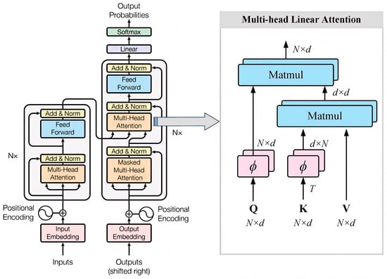
Figure 4. The architecture of the Transformer model with multi-head linear attention.

The Transformer network model consists of two main components: an encoder and a decoder. The encoder maps the input data into a hidden representation, while the decoder transforms this representation into an output sequence. The left side of Figure 4 illustrates the structure of a single encoder layer, and in practice, six identical layers are stacked to enhance the feature representation capability. Correspondingly, the right side depicts the structure of a single decoder layer, which also consists of six identical layers. The decoder output is first processed by a linear transformation layer and then passed through a Softmax layer to generate the final prediction results. Unlike the standard Transformer, the proposed model integrates a multi-head linear attention mechanism within the attention module. By employing kernel function mappings (such as ϕ(Q) and ϕ(K)) to approximate the original attention distribution, the model maintains strong long-range dependency modeling capabilities while reducing computational complexity from quadratic to linear. This design significantly improves the efficiency of large-scale sequence processing. Specifically, each encoder layer comprises a multi-head linear self-attention module and a position-wise feedforward network, while each decoder layer integrates multi-head linear self-attention, multi-head cross-attention, and a feedforward network to enhance contextual feature modeling and information interaction.

The core component of the Transformer network model is the attention mechanism unit. This module encodes the input data into a set of n-dimensional key–value pairs (K and V) to capture dependencies among elements within the sequence. In this study, an improved linear attention mechanism is employed, where a feature mapping function (e.g., ϕ(x) = ELU(x) + 1) projects the query Q and key K into a non-negative space as a replacement for the Softmax operation. This transformation reduces the quadratic computational complexity of the original scaled dot-product attention to a linear form, thereby enabling more efficient spatiotemporal dependency modeling. The computational formulation is expressed as follows:

$$\mathrm{Attention}\left(Q,K,V\right) = {\displaystyle \frac{\mathsf{\varphi }\left(Q\right)\left[\mathsf{\varphi }{\left(K\right)}^{T}V\right]}{\mathsf{\varphi }\left(Q\right)\left[\mathsf{\varphi }{\left(K\right)}^T\mathbf{1}\right]}}$$

(13)

In the implementation, the mapping function ϕ(x) = ELU(x) + 1 possesses non-negativity, differentiability, and an exponential decay property, which enhance the robustness of the attention mechanism under sudden noise fluctuations and anomalous observations. Compared with other mapping functions such as ReLU, Softplus, and Tanh, ELU exhibits superior numerical stability and filtering adaptability when modeling noise in long sequences—making it particularly suitable for dynamic noise covariance estimation in degraded or obstructed GNSS signal environments.

The Transformer architecture was originally developed for natural language processing tasks such as machine translation, text summarization, and speech recognition. In standard models, input data are typically processed through an embedding layer and a positional encoding layer to represent sequence features. However, in the real-time navigation scenario considered in this work, these components are unnecessary. Therefore, the network is customized by retaining the core architecture while removing the embedding and positional encoding layers. Moreover, the traditional scaled dot-product attention is replaced by a multi-head linear attention mechanism, which not only reduces temporal and spatial complexity but also maintains effective long-term dependency modeling under large-scale observational conditions.

In the proposed network design, the inputs include key GNSS observables such as satellite position, satellite velocity, receiver clock bias, azimuth angle, and elevation angle. The model output is a vector a, which is used to dynamically adjust the measurement noise covariance matrix R. The adjustment is defined as follows:

$${\mathrm{R}}^{\prime }={\mathrm{e}}^{\mathsf{\alpha }}\cdot \mathrm{R}$$

(14)

During the training process, the Mean Absolute Error (MAE) is employed as the loss function to quantify the discrepancy between the predicted and true measurement noise covariance values. The expression is given as follows:

$$\mathrm{Loss} = {\displaystyle \frac{1}{\mathrm{n}}}{\sum }_{\mathrm{i}=1}^{\mathrm{n}}\left|{\lambda }_{\mathrm{i}}^{\prime }-{\lambda }_{\mathrm{i}}\right|$$

(15)

Here, ${\lambda }_{\mathrm{i}}^{\prime }$ and ${\lambda }_{\mathrm{i}}$ denote the estimated position coordinates produced by the network and the corresponding ground-truth reference coordinates, respectively. The latter are obtained from high-precision ground-based equipment to provide a reliable supervisory signal.

To further enhance the network’s capability of feature selection along the channel dimension, a Lightweight Residual Channel Attention Module (LRCAM) is integrated into the Transformer backbone. This module is designed to improve the sensitivity of each channel to key measurement noise features. Without altering the original input–output structure of the network, it strengthens the discriminative ability of feature channels and improves the overall robustness of the model, making it particularly suitable for the real-time and lightweight requirements of GNSS/INS tightly coupled navigation systems.

The structure of the LRCAM module consists of the following three steps:

(1)

Channel-wise Pooling:

First, the Transformer output feature matrix $X\in {\mathrm{R}}^{C\times T}$ undergoes average pooling along the channel dimension to obtain the global channel representation vector:

$$Z_c = {\mathrm{AvgPool}}_{\mathrm{channel}}\left(X\right)$$

(16)

Here, C represents the observation feature dimension of each satellite (e.g., position, velocity, clock bias, azimuth, and elevation), and T denotes the number of visible satellites at the current epoch, typically ranging from 6 to 12.

(2)

Lightweight MLP:

The channel representation vector $Z_c$ is then passed through a two-layer lightweight multilayer perceptron (MLP) to perform nonlinear projection and generate the channel attention weights:

$$W_c = \sigma \left(\mathrm{MLP}\left(Z_c\right)\right) = \sigma \left(W_2\mathrm{ReLU}\left(W_1{Z}_c\right)\right)$$

(17)

where W₁ ∈ R^d×C and W₂ ∈ R^C×d, with d = C/r being the reduction ratio (commonly 8 or 16). The activation function σ(⋅) is chosen as the Sigmoid function to achieve normalized weighting across channels.

(3)

Residual Connection:

The channel attention weights $W_c$ are applied to the original features $X$, and a residual connection is used to preserve information continuity, yielding the final reweighted feature representation:

$$X^{\prime }=X\oplus (X\otimes W_c)$$

(18)

Here, $\oplus$ denotes element-wise addition, and $\otimes$ denotes channel-wise element-wise multiplication.

Through this design, the LRCAM module dynamically emphasizes significant channels while leveraging the residual connection to maintain stability. It effectively enhances feature representation capability, suppresses redundant information, and strengthens robustness against noise and outliers. Additionally, when integrated with the preceding R-SDAE and Transformer modules, it forms a unified end-to-end learning framework. This framework improves both the precision of measurement noise covariance estimation and the robustness of navigation filtering. The overall structure of the LRCAM module is illustrated in Figure 5.

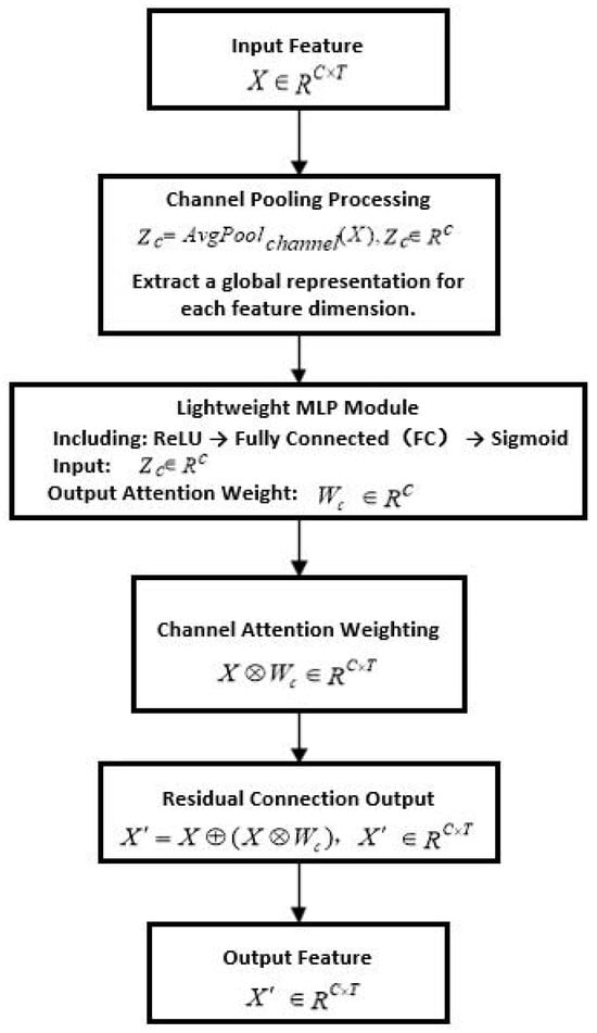
Figure 5. Flowchart of the LRCAM module structure.

3. Results

3.1. Equipment Installation and Data Acquisition

To evaluate the navigation performance of the proposed RLL-AKF algorithm under conditions of GNSS signal blockage or instability, experiments were carried out on 12 October 2022, along representative urban roads in Beijing, China. Data were collected using a ground vehicle equipped with an Xsens MTi-680G GNSS/INS module (Xsens Technologies B.V., Enschede, The Netherlands). The campaign recorded high-rate raw IMU data and GNSS observations. Figure 6 shows the installation layout of the sensors. In our setup, the MTi-680G fuses a high-precision MEMS IMU with GNSS aiding and supports tightly coupled GNSS/INS integration, delivering reliable navigation outputs under complex environments with signal occlusions. The instruments employed and their key specifications are summarized in Table 1. It should be noted that the listed GNSS position RMS of 1 m refers to the nominal standalone open-sky specification of the sensor module, rather than the positioning accuracy achieved in the degraded urban environments considered in this study.

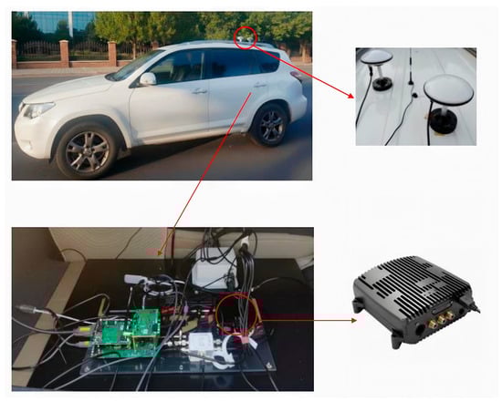
Figure 6. Experimental hardware installation layout.

Table 1. Sensor suite and key performance specifications.

Sensor Module	Specification Item	Rated Value
MTi-680G (INS/IMU)	Gyro bias stability (in-run, 1σ)	8°/h
	Gyro ARW	0.12°/sqrt(h)
	Gyro full-scale range	±100°/s
	Accel bias stability (in-run, 1σ)	0.2 mg
	Accel VRW	0.09 m/s/sqrt(h)
	Acceleration full-scale	±5 g
	IMU output rate	200 Hz
GNSS	GNSS position RMS (nominal, open-sky)	1 m
	GNSS update rate	1 Hz

3.2. Experimental Configuration and Trajectory Design

To verify the effectiveness of the proposed RLL-AKF algorithm, two data segments from the vehicle-mounted navigation system dataset were selected as experimental samples. As shown in Figure 7, within the 1012 dataset, the data segment from 11,000 to 13,500 s was used as the training set (black trajectory), while the segment from 13,500 to 16,000 s served as the testing set (red trajectory). Additionally, the entire trajectory of the 1106 dataset was marked with a red line and used as an independent testing set.

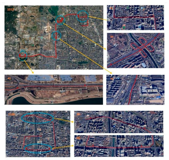
Figure 7. Experimental road trajectories from datasets 1012 and 1106.

In the 1012 dataset, a long-duration section covering both main roads and elevated highways (segment #0, 500 s) was selected to evaluate the adaptability of different neural network-based methods in complex scenarios. Furthermore, four representative challenging segments (#1–#4) were selected and highlighted with blue circles to further assess algorithmic performance. Specifically, Segment #1 corresponds to a scenario with only one or two visible satellites, degraded signal quality, and significant positioning errors. Segment #2 represents a typical urban canyon, surrounded by tall buildings that severely degrade GNSS signal reception. Segment #3 corresponds to a tree-lined avenue, where dense foliage leads to additional observation errors. Segment #4 represents an elevated highway section, where frequent ascending and descending ramps highlight the navigation system’s adaptability under dynamically changing signal conditions. Table 2 summarizes the start and end times, durations, and environmental descriptions of these complex segments to facilitate reproducibility and performance comparison. In the 1106 dataset, two additional segments (#5 and #6) were selected for testing, both representing urban canyon environments characterized by dense high-rise buildings and severe satellite signal blockage. Experimental results across different datasets and diverse environmental conditions demonstrate that the proposed RLL-AKF algorithm consistently maintains high stability and robustness, achieving superior navigation accuracy under challenging scenarios.

Table 2. Seven data segments of complex scenarios.

Dataset Name	Segment ID	Start–End Time (s)	Segment Length (s)	Complex Environment	$\mathbf{Available} \mathbf{Satellites}, {\mathit{N}}_{\mathbf{u}\mathbf{s}\mathbf{e}\mathbf{d}}$ (Mean/Min)	$\mathit{C}/{\mathit{N}}_0$ (Mean/P10, dB-Hz)
Dataset 1012	#0	14,500–15,000	500	Extended road section covering main avenues and viaducts	14/9	38/30
	#1	14,000–14,100	100	Limited satellite visibility with poor-quality signals, leading to large errors	2/1	24/16
	#2	15,800–15,900	100	Urban canyon with dense high-rise buildings	9/4	28/20
	#3	14,500–14,600	100	Tree-lined section where foliage introduces signal interference	11/7	34/26
	#4	14,800–14,900	100	Viaduct section characterized by continuous vehicle turns	11/6	33/24
Dataset 1106	#5	326,000–326,200	200	Low-speed driving in an urban canyon with intermittent satellite blockage and moderate multipath interference	10/6	32/24
	#6	328,100–328,250	150	Urban canyon segment with high building density and severe multipath effects	8/4	29/21

Notes: 1. $N_{\mathrm{u}s\mathrm{e}\mathrm{d}}$ denotes the number of satellites participating in the GNSS/INS tightly coupled solution at each epoch, i.e., those involved in the measurement update and innovation/residual formation. For each road segment, the values are summarized over all epochs as the mean and minimum. 2. $C/N_0$ denotes the carrier-to-noise-density ratio. For each epoch, the average $C/N_0$ of the satellites participating in the solution is computed, and the values for each road segment are summarized as the mean and the 10th percentile (P10), in dB-Hz. 3. The symbol “#” in the Segment ID column (e.g., #0, #1, …, #6) denotes the segment number.

The proposed algorithm was implemented using the PyTorch 1.7 framework. To evaluate its performance in terms of navigation and positioning accuracy, a 500 s road segment was selected from the testing dataset, and its statistical positioning errors were analyzed, as shown in Figure 8.

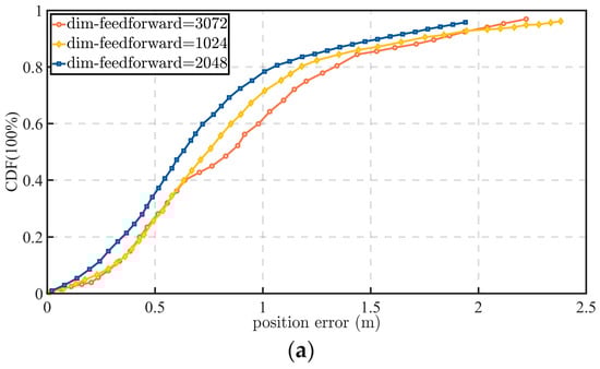
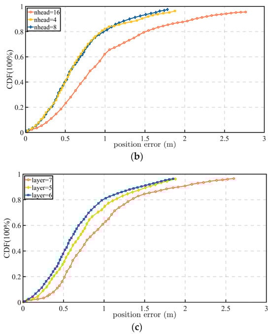
Figure 8. Statistical positioning errors under various hyperparameter configurations: (a) errors under different feedforward layer dimensions; (b) errors under different numbers of attention heads; (c) errors under varying network depth expressed in layer counts.

For the experimental setup, the network hyperparameters were configured as follows: the dropout probability was set to 0.45, the learning rate to 0.0001, and the number of training epochs to 180. The Transformer network consisted of six layers, each incorporating a multi-head attention mechanism with eight heads. To enhance the efficiency of long-sequence feature modeling, the attention module adopted a linear attention structure, reducing its computational complexity to O(n). Parameter optimization was performed using the Adam optimizer to ensure stable convergence during training. The selections of six layers and eight attention heads were determined empirically based on the hyperparameter comparisons in Figure 8. Among the tested configurations, this setting provided the most favorable trade-off between positioning accuracy, error stability, and computational cost; using fewer layers or heads weakened the model capacity for capturing inter-satellite spatiotemporal dependencies, whereas further increasing the model size did not yield sufficiently significant performance gains to justify the additional complexity.

3.3. Comparative Experiments of Different Network Models

To evaluate the performance differences among various network architectures in tightly coupled integrated navigation, a series of comparative experiments was conducted on a representative road segment, focusing primarily on positioning accuracy and stability. The compared models include the following four categories:

(1)

LSTM Model: The Long Short-Term Memory (LSTM) network mitigates the short-term dependency problem inherent in traditional RNNs through gated mechanisms and memory cells. In this experiment, satellite ephemeris data were used as inputs to capture temporal dependencies.

(2)

CNN Model: The Convolutional Neural Network (CNN) extracts local spatial features through convolutional operations. In this study, it was employed to derive informative features from satellite ephemeris data and estimate the measurement noise covariance matrix R.

(3)

Transformer Model: As detailed in Section 2.4, the standard Transformer exhibits strong capabilities in long-term dependency modeling and attention-based feature extraction.

(4)

RLL Model (R-SDAE + Linear Attention + LRCAM): The proposed model enhances the standard Transformer framework by integrating three optimization modules. The Residual Sparse Denoising Autoencoder (R-SDAE) performs denoising on input data to extract robust sparse features. The Linear Attention mechanism maintains global dependency modeling while significantly reducing computational complexity. The Lightweight Residual Channel Attention Module (LRCAM) recalibrates channel-wise features, reinforcing the response to key noise-related characteristics. The combined effect of these modules yields superior robustness and generalization in multi-interference environments.

To ensure fairness in comparison, the experiment selected Segment #0 from Figure 7, a 500 s road section that includes both tree-lined avenues and overpasses, representing typical complex urban conditions. The positioning error results of each model on this segment are shown in Figure 9.

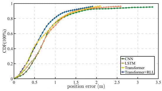
Figure 9. Position errors of tightly coupled GNSS/INS navigation with the measurement-noise covariance R estimated by different neural networks.

The results indicate that the proposed RLL model achieves the best overall performance among the compared neural covariance estimators. In this study, the CNN and LSTM models serve as representative convolutional and recurrent baselines, while the standard Transformer serves as an attention-based baseline for measurement-noise covariance prediction. Relative to these models, the proposed RLL model yields lower positioning errors and smoother error evolution on Segment #0, indicating that the combination of R-SDAE, Linear Attention, and LRCAM improves both robustness to corrupted observations and the stability of covariance estimation. These results show that the proposed design provides a more favorable accuracy–robustness trade-off than the compared deep-learning covariance estimators considered in this work.

3.4. Computational Cost Evaluation of Different Network Models

To further assess the practical deployment cost of the proposed covariance estimator, Table 3 reports the parameter count, training time, and per-epoch prediction time of the evaluated neural models on a platform equipped with an NVIDIA GeForce GTX 1650 GPU, an Intel(R) Core(TM) i7-8750H CPU (2.20 GHz), and 16 GB of RAM. The compared models cover representative deep learning paradigms for covariance estimation, including convolutional (CNN), recurrent (LSTM), and attention-based architectures, while the proposed RLL model further integrates R-SDAE and LRCAM on top of the Transformer backbone.

Table 3. Complexity and runtime statistics of the evaluated models.

Model	Parameter Count	Training Time (s)	Prediction Time (ms)
LSTM	157,696	41.78	1.12
CNN	21,026	26.82	1.05
R-SDAE	25,820	92.00	–
RLL	1,660,100	286.00	15.20

As shown in Table 3, the proposed RLL model contains 1,660,100 parameters and requires 15.20 ms per prediction, whereas the LSTM and CNN baselines require 1.12 ms and 1.05 ms, respectively. This increase in runtime reflects the additional cost introduced by residual sparse denoising and attention-enhanced feature recalibration, but it is accompanied by the best positioning accuracy among the compared neural covariance estimators in Section 3.3. To provide a deployment-oriented interpretation, the GNSS measurement-update rate in the present system is 1 Hz, corresponding to 1000 ms per epoch, whereas the inertial propagation runs at 200 Hz. Therefore, the proposed covariance predictor is invoked only at the GNSS measurement-update stage rather than at every inertial mechanization step. Under this operating mode, the measured inference time of 15.20 ms accounts for approximately 1.52% of one GNSS update interval on the desktop platform, indicating a sufficient timing margin for real-time covariance prediction within the EKF update loop. In addition, the network parameters are optimized offline during model development, whereas online deployment requires only forward prediction of the measurement-noise covariance and EKF updating. In practical terms, the current model is more suitable for vehicle-mounted industrial computers or edge-assisted computing units than for highly resource-constrained low-power embedded processors. It should also be emphasized that this comparison does not constitute a dedicated embedded benchmark, because the processor architecture, memory bandwidth, and system-level scheduling overhead may alter the actual runtime on onboard hardware. Future work will therefore evaluate the proposed model on representative embedded platforms and investigate quantization, pruning, and hardware-aware optimization to further reduce latency and the memory footprint for resource-constrained deployment.

3.5. Comparative Experiments of Different Methods

To validate the effectiveness of the proposed RLL-AKF method, comparative experiments were conducted against three representative benchmark filters. The evaluated methods are as follows:

(1)

RLL-AKF: The proposed approach integrates three enhancement modules within the Transformer backbone. The Residual Sparse Denoising Autoencoder (R-SDAE) performs sparse feature denoising, Linear Attention reduces computational complexity while preserving long-sequence dependency modeling, and the Lightweight Residual Channel Attention Module (LRCAM) dynamically recalibrates critical channel features. Together, these components significantly improve the accuracy and robustness of measurement noise covariance estimation.

(2)

C-KF: A Conventional Kalman Filter assuming a fixed measurement noise covariance matrix throughout the filtering process.

(3)

AF-AKF: The Adaptive Fading Memory Kalman Filter, which introduces a fading factor into the gain computation to dynamically modulate the influence of historical information on current estimates. This mechanism enhances adaptability under nonstationary and burst-noise conditions.

(4)

I-AKF: The Innovation-Based Adaptive Kalman Filter, which adaptively adjusts the measurement noise covariance matrix based on innovation statistics, dynamically correcting the filtering process in response to variations in observation residuals [39].

In the dataset 1012, four 100 s road segments were selected as test samples to evaluate the filter performance. To further assess the generalization capability of the model under diverse environmental conditions, two additional road segments—lasting 200 s and 150 s, respectively—were extracted from the dataset 1106 as supplementary test samples.

The comparative evaluation employed four statistical indicators: maximum error (MAX), minimum error (MIN), mean error (µ), and error variance (σ²), to comprehensively assess the positioning accuracy of each method. The quantitative results are summarized in Table 4, Table 5, Table 6, Table 7, Table 8 and Table 9. For a more intuitive understanding, the positioning error curves and accuracy comparison plots are also provided below, clearly illustrating the performance advantages of the proposed RLL-AKF approach over conventional methods.

Table 4. Position error comparison in Segment #1 across different algorithms.

Strategy	Position Error (m)
	MAX	MIN	µ	σ2
C-KF	46.65	4.20	16.17	79.50
AF-AKF	48.27	1.86	15.28	72.06
I-AKF	85.76	3.67	51.42	346.25
RLL-AKF	11.20	0.24	3.18	11.28

Table 5. Position error comparison in Segment #2 across different algorithms.

Strategy	Position Error (m)
	MAX	MIN	µ	σ2
C-KF	6.82	0.78	2.50	2.26
AF-AKF	6.54	0.38	2.28	2.02
I-AKF	14.20	0.67	4.56	20.80
RLL-AKF	5.88	0.30	1.62	1.76

Table 6. Position error comparison in Segment #3 across different algorithms.

Strategy	Position Error (m)
	MAX	MIN	µ	σ2
C-KF	2.66	0.28	1.42	0.86
AF-AKF	2.45	0.22	0.96	0.23
I-AKF	2.99	0.25	1.29	0.56
RLL-AKF	1.58	0.16	0.69	0.10

Table 7. Position error comparison in Segment #4 across different algorithms.

Strategy	Position Error (m)
	MAX	MIN	µ	σ2
C-KF	4.80	0.26	1.60	1.28
AF-AKF	3.29	0.24	1.29	1.23
I-AKF	3.72	0.46	1.38	0.65
RLL-AKF	2.32	0.31	0.98	0.40

Table 8. Position error comparison in Segment #5 across different algorithms.

Strategy	Position Error (m)
	MAX	MIN	µ	σ2
C-KF	6.50	2.55	4.80	0.76
AF-AKF	6.12	2.38	4.36	0.63
I-AKF	8.10	1.82	5.82	0.66
RLL-AKF	4.62	1.52	3.41	0.59

Table 9. Position error comparison in Segment #6 across different algorithms.

Strategy	Position Error (m)
	MAX	MIN	µ	σ2
C-KF	4.58	1.52	2.54	0.80
AF-AKF	4.22	1.45	2.43	0.67
I-AKF	7.86	0.98	2.65	2.32
RLL-AKF	2.79	0.71	1.97	0.38

Road Segment #1 represents a typical challenging scenario in which only 1–2 satellites are visible, resulting in a significant degradation of overall positioning accuracy. As shown in Figure 10 and Figure 11, the proposed RLL-AKF method achieves the best performance among the four algorithms. In comparison, the AF-AKF method exhibits a certain error suppression capability under such conditions but still lags behind RLL-AKF in both accuracy and stability. The C-KF method performs at a moderately low level, while the I-AKF shows the poorest results. Specifically, the maximum positioning error of I-AKF reaches 85.76 m, and its mean error exceeds 51.42 m (see Table 4), indicating insufficient robustness under low satellite visibility. The performance degradation of I-AKF primarily stems from the fact that when the GNSS signal quality is severely degraded, its innovation-based adaptive noise covariance adjustment mechanism tends to fail, leading to a significant increase in estimation bias. In contrast, the proposed RLL-AKF maintains remarkable stability under the same conditions, achieving a mean error of only 3.18 m and a minimum error of 0.24 m, outperforming all comparison methods. These results clearly demonstrate the superior robustness of the proposed approach in complex observation environments.

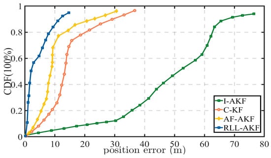
Figure 10. Comparative accuracy of different methods in Segment #1.

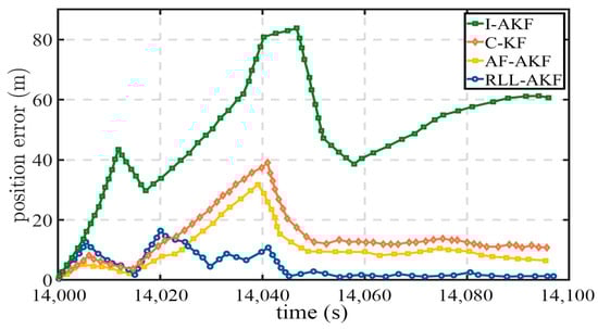
Figure 11. Position error comparison in Segment #1 for tightly coupled GNSS/INS using different algorithms.

Road Segment #2 corresponds to a typical urban canyon environment, where dense high-rise buildings cause severe interference with GNSS signal reception. As observed from Figure 12 and Figure 13, the overall positioning error in this segment is higher than in other sections, primarily due to the signal obstruction caused by reduced satellite visibility. Under these conditions, the I-AKF method shows a sharp increase in error, with a maximum value of 14.20 m, indicating a significant drop in positioning accuracy. In contrast, the proposed RLL-AKF method demonstrates greater stability and robustness in the same challenging conditions, achieving a mean error of only 1.62 m and a minimum error of 0.30 m (see Table 5). Overall, the RLL-AKF consistently outperforms other comparison methods, verifying its superior adaptability and reliability in urban canyon scenarios.

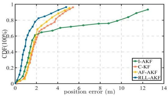
Figure 12. Comparative accuracy of different methods in Segment #2.

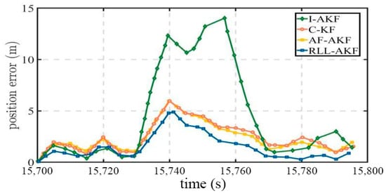
Figure 13. Position error comparison in Segment #2 for tightly coupled GNSS/INS using different algorithms.

Road Segment #3 corresponds to a tree-lined roadway, where tall trees introduce additional interference to GNSS signal reception. As shown in Figure 14, the proposed RLL-AKF method achieves significantly higher positioning accuracy at the 67% confidence level compared with both AF-AKF and I-AKF, and it also outperforms the C-KF method. It is worth noting that although I-AKF exhibits a larger maximum positioning error than the other algorithms in this scenario, its mean error is not the highest. In contrast, the C-KF method records the largest mean error and error variance among all four algorithms, indicating greater fluctuations in positioning performance and insufficient robustness under the tree-lined environment, as illustrated in Figure 15 and Table 6.

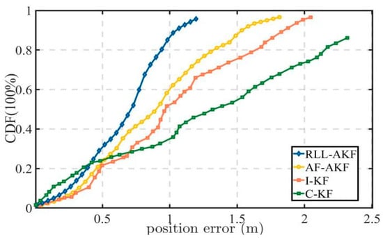
Figure 14. Comparative accuracy of different methods in Segment #3.

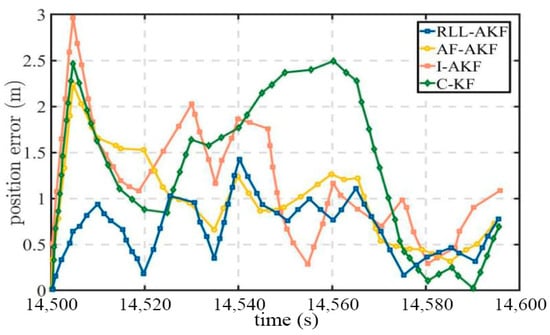
Figure 15. Position error comparison in Segment #3 for tightly coupled GNSS/INS using different algorithms.

Road Segment #4 corresponds to an overpass scenario, where the vehicle performs multiple turns while ascending and descending the bridge, fully reflecting the susceptibility of satellite signals to obstruction in such environments. As shown in Table 7, the four methods exhibit relatively small differences in their maximum and minimum errors, yet the RLL-AKF method achieves the best performance in terms of both mean error and variance. From the results in Figure 16 and Figure 17, it can be observed that at the 67% confidence level, the accuracy of AF-AKF, C-KF, and I-AKF is generally comparable to that of RLL-AKF. However, at the 90% confidence level, the I-AKF method’s error increases sharply, diverging to approximately 2.94 m. Moreover, C-KF exhibits maximum errors exceeding 4.00 m at certain time points, indicating poorer stability under the complex bridge environment.

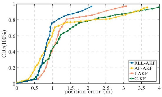
Figure 16. Comparative accuracy of different methods in Segment #4.

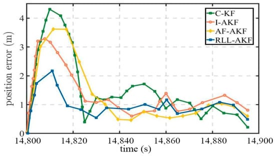
Figure 17. Position error comparison in Segment #4 for tightly coupled GNSS/INS using different algorithms.

Road Segment #5 represents a typical urban canyon environment with a duration of 200 s, where the vehicle moves at low speed, and the satellite signals are frequently obstructed by surrounding high-rise buildings. As shown in Table 8, the proposed RLL-AKF method achieves both lower maximum and minimum positioning errors compared to the other three traditional methods, with an average error of 3.41 m, which is significantly lower than that of the alternatives. From the results illustrated in Figure 18 and Figure 19, it can be observed that the proposed RLL-AKF method consistently outperforms the other approaches throughout the entire route segment. Due to the poor satellite signal quality, the I-AKF method exhibits the worst performance, with errors increasing markedly. These results further validate the robustness and reliability advantages of the proposed method under complex and weak-signal conditions.

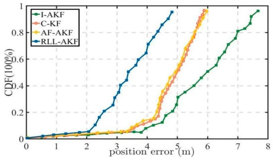
Figure 18. Comparative accuracy of different methods in Segment #5.

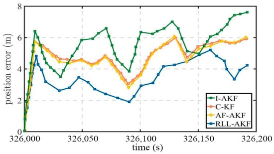
Figure 19. Position error comparison in Segment #5 for tightly coupled GNSS/INS using different algorithms.

Road Segment #6 corresponds to an urban canyon densely surrounded by high-rise buildings, where the GNSS signals suffer from severe blockage and are affected by significant multipath errors. As presented in Table 9, the proposed RLL-AKF method achieves the lowest mean positioning error among the four compared algorithms. Furthermore, as shown in Figure 20 and Figure 21, the proposed method demonstrates superior overall performance, with a maximum positioning error of only 2.76 m, which is notably smaller than that of the other methods. Considering the experimental results from Segments #5 and #6, it can be concluded that the proposed method maintains a stable performance under various signal blockage conditions, exhibiting strong robustness and adaptability, while also demonstrating significant advantages in noise modeling and high-precision positioning.

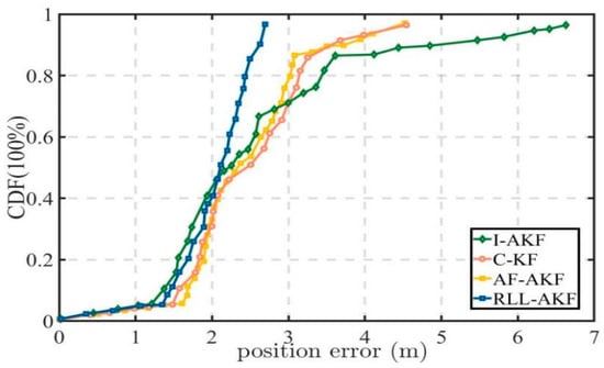
Figure 20. Comparative accuracy of different methods in Segment #6.

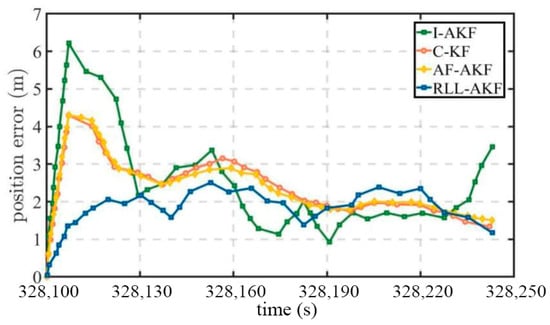
Figure 21. Position error comparison of tightly coupled GNSS/INS using different methods in Segment #6.

4. Discussion

The experimental results demonstrate that the proposed RLL-AKF method achieves a superior performance across the evaluated urban road scenarios and the considered comparison methods. In addition to the comparisons with conventional adaptive filtering approaches, Section 3.3 further evaluates the proposed estimator against representative neural covariance predictors, including CNN, LSTM, and the standard Transformer. The proposed RLL design provides the most favorable balance between positioning accuracy and error stability, indicating that residual sparse denoising, linear-complexity attention, and channel recalibration play complementary roles in covariance prediction under degraded GNSS conditions. From the deployment perspective, the measured prediction time is 15.20 ms on the desktop platform used in this study. Relative to the 1 Hz GNSS measurement-update rate of the current system, this corresponds to approximately 1.52% of one update interval, suggesting that the proposed model has a sufficient timing margin for real-time covariance estimation at the measurement-update stage on desktop or edge-assisted platforms. Nevertheless, several limitations should be acknowledged. First, the end-to-end training procedure relies on RTK-fixed or equivalent high-precision reference trajectories as supervision, and the current framework is therefore most suitable for settings in which such reference data are available during model development. Moreover, these references should be regarded as practical high-precision supervision rather than exact ground truth, because residual uncertainty may still arise from satellite geometry, multipath, ambiguity fixing, and time synchronization, thereby introducing a certain level of label noise into network training. Second, although validation on independent road segments indicates a certain degree of environmental transferability, all experiments in this study were conducted on the same vehicle-mounted GNSS/INS platform, and the generalization of the proposed model to unseen sensor configurations, IMU grades, antenna layouts, sampling rates, and GNSS front-end characteristics has not yet been systematically evaluated. Third, the current timing analysis is based on desktop measurements rather than dedicated embedded benchmarking; the actual onboard runtime may vary with processor capability, memory bandwidth, and software scheduling overhead. These issues will be addressed in future work through weakly supervised or self-supervised covariance learning, cross-platform adaptation, and hardware-aware model compression and acceleration for resource-constrained onboard deployment [40].

5. Conclusions

This study addresses the challenge of modeling measurement noise statistics in dynamic environments by proposing an adaptive noise covariance estimation algorithm (RLL-AKF) that integrates a Residual Sparse Denoising Autoencoder (R-SDAE), Linear Attention, and a Lightweight Residual Channel Attention Module (LRCAM). Within the Transformer framework, the R-SDAE enhances denoising and robust feature extraction from noisy observations; the Linear Attention mechanism enables efficient long-term dependency modeling while significantly reducing computational complexity; and the LRCAM dynamically recalibrates critical feature channels to strengthen feature representation. The synergy of these three components leads to a comprehensive improvement in the accuracy and stability of noise covariance estimation.

Compared with traditional adaptive filtering methods, the proposed RLL-AKF achieves a higher positioning accuracy and stronger robustness on the evaluated GNSS-degraded road-test datasets. Extensive experiments across multiple challenging segments show that the proposed algorithm maintains a superior filtering performance under severe signal degradation, and in representative difficult scenarios, it reduces the mean positioning error to approximately 3.4 m. At the same time, the present study has several limitations. Model training depends on RTK-quality reference trajectories, and the current validation is confined to the vehicle-mounted sensor configuration and data collection setting used in this work. Accordingly, the generalization of the proposed model to unseen sensor suites, hardware grades, and operating conditions remains to be further verified. Future work will focus on reducing the dependence on high-precision labels, extending validation to heterogeneous platforms, and improving deployment efficiency on embedded hardware.

References

- Titterton, D.H.; Weston, J.L. Strapdown Inertial Navigation Technology, 2nd ed.; Institution of Electrical Engineers: Stevenage, UK, 2004. [Google Scholar]
- Groves, P.D. Principles of GNSS, Inertial, and Multisensor Integrated Navigation Systems, 2nd ed.; Artech House: Boston, MA, USA, 2013. [Google Scholar]
- Noureldin, A.; Karamat, T.B.; Eberts, M.D.; El-Shafie, A. Performance Enhancement of MEMS-Based INS/GPS Integration for Low-Cost Navigation Applications. IEEE Trans. Veh. Technol. 2009, 58, 1077–1096. [Google Scholar] [CrossRef]
- Skog, I.; Handel, P. In-Car Positioning and Navigation Technologies—A Survey. IEEE Trans. Intell. Transp. Syst. 2009, 10, 4–21. [Google Scholar] [CrossRef]
- Liu, H.; Nassar, S.; El-Sheimy, N. Two-Filter Smoothing for Accurate INS/GPS Land-Vehicle Navigation in Urban Centers. IEEE Trans. Veh. Technol. 2010, 59, 4256–4267. [Google Scholar] [CrossRef]
- Bar-Shalom, Y.; Li, X.-R.; Kirubarajan, T. Estimation with Applications to Tracking and Navigation: Theory, Algorithms, and Software; John Wiley & Sons: New York, NY, USA, 2001. [Google Scholar]
- Grejner-Brzezinska, D.A.; Toth, C.K.; Sun, H.; Wang, X.; Rizos, C. A Robust Solution to High-Accuracy Geolocation: Quadruple Integration of GPS, IMU, Pseudolite, and Terrestrial Laser Scanning. IEEE Trans. Instrum. Meas. 2011, 60, 3694–3708. [Google Scholar] [CrossRef]
- Hu, G.; Gao, S.; Zhong, Y. A Derivative UKF for Tightly Coupled INS/GPS Integrated Navigation. ISA Trans. 2015, 56, 135–144. [Google Scholar] [CrossRef] [PubMed]
- Han, H.; Wang, J.; Du, M. GPS/BDS/INS Tightly Coupled Integration Accuracy Improvement Using an Improved Adaptive Interacting Multiple Model with Classified Measurement Update. Chin. J. Aeronaut. 2018, 31, 556–566. [Google Scholar] [CrossRef]
- Peyraud, S.; Bétaille, D.; Renault, S.; Ortiz, M.; Mougel, F.; Meizel, D.; Peyret, F. About Non-Line-of-Sight Satellite Detection and Exclusion in a 3D Map-Aided Localization Algorithm. Sensors 2013, 13, 829–847. [Google Scholar] [CrossRef] [PubMed]
- Dhital, A.; Lachapelle, G.; Bancroft, J.B. Improving the Reliability of Personal Navigation Devices in Harsh Environments. In Proceedings of the 2015 International Conference on Indoor Positioning and Indoor Navigation (IPIN), Banff, AB, Canada, 13–16 October 2015; pp. 1–7. [Google Scholar] [CrossRef]
- Huang, Y.; Zhang, Y.; Wu, Z.; Li, N.; Chambers, J.A. A Novel Adaptive Kalman Filter with Inaccurate Process and Measurement Noise Covariance Matrices. IEEE Trans. Autom. Control 2018, 63, 594–601. [Google Scholar] [CrossRef]
- Katharopoulos, A.; Vyas, A.; Pappas, N.; Fleuret, F. Transformers Are RNNs: Fast Autoregressive Transformers with Linear Attention. In Proceedings of the 37th International Conference on Machine Learning, Virtual Event, 13–18 July 2020; pp. 5156–5165. [Google Scholar]
- Mehra, R.K. On the Identification of Variances and Adaptive Kalman Filtering. IEEE Trans. Autom. Control 1970, 15, 175–184. [Google Scholar] [CrossRef]
- Meng, Y.; Gao, S.; Zhong, Y.; Hu, G.; Šubić, A. Covariance Matching-Based Adaptive Unscented Kalman Filter for Direct Filtering in INS/GNSS Integration. Acta Astronaut. 2016, 120, 171–181. [Google Scholar] [CrossRef]
- Cho, S.Y.; Choi, W.S. A Robust Positioning Technique in DR/GPS Using the Receding Horizon Sigma Point Kalman FIR Filter. In Proceedings of the IEEE Instrumentation and Measurement Technology Conference (IMTC 2005), Ottawa, ON, Canada, 17-19 May 2005; IEEE: New York, NY, USA, 2005; Volume 2, pp. 1354–1359. [Google Scholar] [CrossRef]
- Zhang, H.; Chang, Y.H.; Che, H. Measurement-Based Adaptive Kalman Filtering Algorithm for GPS/INS Integrated Navigation System. J. Chin. Inert. Technol. 2010, 18, 696–701. [Google Scholar]
- Xu, S.; Zhou, H.; Wang, J.; He, Z.; Wang, D. SINS/CNS/GNSS Integrated Navigation Based on an Improved Federated Sage–Husa Adaptive Filter. Sensors 2019, 19, 3812. [Google Scholar] [CrossRef] [PubMed]
- Ge, B.; Zhang, H.; Jiang, L.; Li, Z.; Butt, M.M. Adaptive Unscented Kalman Filter for Target Tracking with Unknown Time-Varying Noise Covariance. Sensors 2019, 19, 1371. [Google Scholar] [CrossRef] [PubMed]
- Hide, C.; Moore, T.; Smith, M. Adaptive Kalman Filtering for Low-Cost INS/GPS. J. Navig. 2003, 56, 143–152. [Google Scholar] [CrossRef]
- Ge, B.; Zhang, H.; Fu, W.; Yang, J. Enhanced Redundant Measurement-Based Kalman Filter for Measurement Noise Covariance Estimation in INS/GNSS Integration. Remote Sens. 2020, 12, 3500. [Google Scholar] [CrossRef]
- Bavdekar, V.A.; Deshpande, A.P.; Patwardhan, S.C. Identification of Process and Measurement Noise Covariance for State and Parameter Estimation Using Extended Kalman Filter. J. Process Control 2011, 21, 585–601. [Google Scholar] [CrossRef]
- Sun, R.; Zhang, Z.; Cheng, Q.; Ochieng, W.Y. Pseudorange Error Prediction for Adaptive Tightly Coupled GNSS/IMU Navigation in Urban Areas. GPS Solut. 2022, 26, 28. [Google Scholar] [CrossRef]
- Or, B.; Klein, I. A Hybrid Model and Learning-Based Adaptive Navigation Filter. IEEE Trans. Instrum. Meas. 2022, 71, 2516311. [Google Scholar] [CrossRef]
- Julier, S.J.; Uhlmann, J.K. Unscented Filtering and Nonlinear Estimation. Proc. IEEE 2004, 92, 401–422. [Google Scholar] [CrossRef]
- Song, J.; Li, J.; Wei, X.; Hu, C.; Zhang, Z.; Zhao, L.; Jiao, Y. Improved Multiple-Model Adaptive Estimation Method for Integrated Navigation with Time-Varying Noise. Sensors 2022, 22, 5976. [Google Scholar] [CrossRef] [PubMed]
- Haarnoja, T.; Ajay, A.; Levine, S.; Abbeel, P. Backprop KF: Learning Discriminative Deterministic State Estimators. In Proceedings of the Advances in Neural Information Processing Systems 29 (NeurIPS 2016), Barcelona, Spain, 5–10 December 2016; pp. 4376–4384. [Google Scholar]
- Revach, G.; Shlezinger, N.; van Sloun, R.J.G.; Eldar, Y.C. KalmanNet: Data-Driven Kalman Filtering. In Proceedings of the IEEE International Conference on Acoustics, Speech and Signal Processing (ICASSP 2021), Toronto, ON, Canada, 6–11 June 2021; pp. 3905–3909. [Google Scholar] [CrossRef]
- Rabby, M.F.; Tu, Y.; Hossen, M.I.; Lee, I.; Maida, A.S.; Hei, X. Stacked LSTM based deep recurrent neural network with kalman smoothing for blood glucose prediction. BMC Med. Inform. Decis. Mak. 2021, 21, 101. [Google Scholar]
- Wu, F.; Luo, H.; Jia, H.; Zhao, F.; Xiao, Y.; Gao, X. Predicting the Noise Covariance with a Multitask Learning Model for Kalman Filter-Based GNSS/INS Integrated Navigation. IEEE Trans. Instrum. Meas. 2021, 70, 8500613. [Google Scholar] [CrossRef]
- Ding, D.; He, K.F.; Qian, W.Q. A Bayesian Adaptive Unscented Kalman Filter for Aircraft Parameter and Noise Estimation. J. Sens. 2021, 2021, 9002643. [Google Scholar] [CrossRef]
- Noureldin, A.; Karamat, T.B.; Georgy, J. Fundamentals of Inertial Navigation, Satellite-Based Positioning and Their Integration; Springer: Berlin/Heidelberg, Germany, 2013. [Google Scholar] [CrossRef]
- Misra, P.; Enge, P. Global Positioning System: Signals, Measurements, and Performance; Ganga-Jamuna Press: Lincoln, MA, USA, 2001. [Google Scholar]
- Chiang, K.-W.; Duong, T.T.; Liao, J.-K. The Performance Analysis of a Real-Time Integrated INS/GPS Vehicle Navigation System with Abnormal GPS Measurement Elimination. Sensors 2013, 13, 10599–10622. [Google Scholar] [CrossRef]
- Anderson, B.D.O.; Moore, J.B. Optimal Filtering; Dover Publications: Mineola, NY, USA, 2005. [Google Scholar]
- Vincent, P.; Larochelle, H.; Bengio, Y.; Manzagol, P.-A. Extracting and Composing Robust Features with Denoising Autoencoders. In Proceedings of the 25th International Conference on Machine Learning (ICML), Helsinki, Finland, 5–9 July 2008; pp. 1096–1103. [Google Scholar] [CrossRef]
- Hochreiter, S.; Schmidhuber, J. Long Short-Term Memory. Neural Comput. 1997, 9, 1735–1780. [Google Scholar] [CrossRef] [PubMed]
- Chaudhari, S.; Mithal, V.; Polatkan, G.; Ramanath, R. An Attentive Survey of Attention Models. ACM Trans. Intell. Syst. Technol. 2021, 12, 53. [Google Scholar] [CrossRef]
- Akhlaghi, S.; Zhou, N.; Huang, Z. Adaptive Adjustment of Noise Covariance in Kalman Filter for Dynamic State Estimation. In Proceedings of the 2017 IEEE Power & Energy Society General Meeting, Chicago, IL, USA, 16–20 July 2017; pp. 1–5. [Google Scholar] [CrossRef]
- Xu, H.; Luo, H.; Wu, Z.; Wu, F.; Bao, L.; Zhao, F. Towards Predicting the Measurement Noise Covariance with a Transformer and Residual Denoising Autoencoder for GNSS/INS Tightly-Coupled Integrated Navigation. Remote Sens. 2022, 14, 1691. [Google Scholar] [CrossRef]
Disclaimer/Publisher’s Note: The statements, opinions and data contained in all publications are solely those of the individual author(s) and contributor(s) and not of MDPI and/or the editor(s). MDPI and/or the editor(s) disclaim responsibility for any injury to people or property resulting from any ideas, methods, instructions or products referred to in the content. |
© 2026 by the authors. Licensee MDPI, Basel, Switzerland. This article is an open access article distributed under the terms and conditions of the Creative Commons Attribution (CC BY) license.