A 3D Structure Extraction Method from Multi-Depth Ocean Temperature Data

Abstract

Understanding subsurface temperature-transition structures is essential for interpreting upper-ocean stratification; however, most existing methods rely on two-dimensional profiles and fail to resolve the full three-dimensional geometry of temperature anomalies. This study proposes the Three-Dimensional Ocean Temperature Structure Extraction method (3D-OTSE), a flexible data-driven framework that identifies coherent three-dimensional thermal-transition features directly from multi-depth ocean temperature fields. The method defines a Temperature-Contrast Index (TCI) based on local three-dimensional temperature differences, determines an adaptive threshold from the curvature of the TCI distribution, and employs 3D DBSCAN to extract volumetric structures. Rather than assuming a thermocline, 3D-OTSE detects a wide range of vertical temperature anomalies—including thermoclines, inverse thermoclines, and multilayer transitions—according to their spatial organization in the data. Applying this method to the South China Sea Basin (SCS) can reconstruct thermocline-like structures that conform to large-scale regional patterns and can also capture complex lateral variations that are difficult to detect by traditional profile diagnosis methods. The region-adaptive threshold enables this framework to adapt to inhomogeneous formation states and spatio-temporal scales. In general, 3D-OTSE provides a universal, parameter-adaptive tool for finding three-dimensional underground temperature anomaly layers, supplements perspectives for traditional methods, and lays the foundation for future multivariate and time-varying applications.

1. Introduction

There are diverse anomalous situations and stratification structures in the temperature of the upper ocean, such as thermoclines, temperature inversions, frontal gradients, and mesoscale anomaly patterns, etc. These structures regulate the stratification, heat storage, and air–sea exchange of the upper ocean. They are recorded through global Argo observations and large-scale subsurface heat variable analysis [1,2]. Recent studies show that such anomalies usually have coherent horizontal extension ranges and are shaped into complex three-dimensional geometric forms by mesoscale dynamics. This suggests that they are spatially continuous volumetric features rather than isolated vertical signatures [3,4]. With the rapid growth of multi-depth in situ observations, numerical simulations, and satellite–Argo fused datasets, data-driven methods now present promising opportunities for reconstructing and interpreting three-dimensional thermal structures directly from observations [5]. In recent decades, a wide range of approaches has been developed to detect and quantify upper-ocean temperature anomalies and stratified structures. Observation-oriented strategies include adaptive sampling with autonomous underwater vehicles, which can detect strong vertical temperature transitions and adjust their trajectories in real time to follow sharp stratified layers [6,7]. Additionally, acoustic and marine seismic reflection techniques have been employed to image fine-scale thermohaline layering in shelf and frontal regions, providing quasi-continuous sections of subsurface structure over mesoscale distances [8].

At the diagnostic level, the most widely used schemes rely on two-dimensional vertical profiles of temperature or density, from which key parameters such as boundary depths, thickness, and intensity of mixed or transition layers are derived. Numerous studies define mixed-layer or stratified-layer depths using fixed temperature or density thresholds, optimal linear fits, maximum-angle criteria, or curvature-based measures [9,10,11,12]. Global or regional climatologies have been constructed based on these profile-based definitions [11,12]. Additionally, other works adopt profile-fitting approaches that utilize S-shaped or hyperbolic-tangent functions to objectively characterize sharp vertical transitions across diverse dynamical regimes [13,14].

Parallel developments have focused on the automatic detection of horizontal temperature anomaly features, such as mesoscale and submesoscale fronts, from satellite sea surface temperature (SST) products. Proposed various algorithms, such as gradient-based, edge detection, histogram threshold, etc., for extracting frontal regions from high-resolution sea surface temperature images and analyzing long-term changes [15,16,17]. Recent studies combine SST data with wind fields inverted by synthetic aperture radar or perform multi-sensor fusion to enhance the robustness and spatial continuity of frontal detection in coastal and marginal seas [18].

Technological advancements enable data-driven techniques to derive subsurface/3D thermal structures from observed data. Super-resolution frameworks, integrated machine learning models, deep neural networks, and generative adversarial network architectures are used to reconstruct subsurface temperature fields from remote sensing data [19], invert 3D temperature–salinity profiles from the combination of satellite and Argo data [20,21,22,23], and also resolve mesoscale/regional thermal anomalies under the vortex-resolving background [21,22,23,24]. Studies on lakes, etc., show that changes in thermocline depth/intensity can affect ecosystems, highlighting the importance of accurately characterizing such anomalous structures [25].

Existing methods are different from each other, and most technologies are restricted by assumptions and dimensions. Profile-based methods dominate in detecting stratification or transition layers, simplifying three-dimensional temperature anomaly changes into a single column to represent. Previous evaluations show that two-dimensional criteria are more sensitive to vertical noise, sampling sparsity, and regional stratification differences, leading to inconsistent detection across spatio-temporal boundaries [26]. Many diagnostic schemes rely on prescribed temperature or density thresholds, fixed gradient criteria, or empirical shape parameters, and the results are particularly dependent on regional dynamic states and data resolution. This limitation has been widely pointed out in comparative studies [27].

Similarly, the algorithms focused on surface fronts primarily describe horizontal gradients and do not naturally extend to subsurface or volumetric structures, which often exhibit complex vertical coherence that cannot be inferred from surface signals alone [28]. Even recent data-driven inversion frameworks typically reconstruct temperature fields either pointwise or profilewise, without providing a unified mechanism for objectively delineating three-dimensional anomaly structures. Therefore, the current method limits the generalization ability across temperature abnormal layers, and still cannot stably characterize the three-dimensional distribution, geometric morphology, or continuity. This difference reflects the mismatch between modern high-resolution three-dimensional temperature data and traditional two-dimensional interpolation analysis tools.

Numerous subsurface temp-trans features such as thermoclines, inversion layers, and mesoscale induced anomalies have three-dimensional structures, and these structures cannot be fully demonstrated by independent two-dimensional profiles. This observation has led to the emergence of a 3D operation form, where the coherent structures originate from the temperature field without pre-setting their vertical forms.

To fill the gap of this method, this study proposes a flexible, data-driven framework named 3D-OTSE to identify temperature anomaly structures from multi-depth temperature fields. 3D-OTSE does not assume the morphology, depth range, or physical origin of specific structures. Instead, it adopts adaptive parameterization, enabling users to adjust sensitivity and spatial scale according to the characteristics of each dataset. This method uses the temperature contrast index (TCI) to quantify local 3D temperature anomalies and also evaluates anomaly significance based on data-adaptive thresholds of the statistical distribution of TCI values. Then, candidate anomaly points are clustered into coherent volume features through a 3D density-based clustering scheme. Through this fully data-driven workflow, 3D-OTSE is a universal anomaly discovery tool that can extract various temperature anomaly structures, such as transition layers, inversion features, and dynamically generated subsurface anomalies, without predetermined structure assumptions. A unified and highly adaptable framework for analyzing the complex three-dimensional thermal characteristics of marine regions, which can also carry out targeted case studies, providing a multi-functional and physically consistent basis.

The rest of the paper is organized as follows. Section 2 illustrates the system architecture and details of 3D-OTSE. Section 3 describes the data used in the experiment, as well as the study area. Section 4 reports the experimental results and Section 5 reports the discussion. Finally, conclusions are presented in Section 6.

2. Methods

This paper proposes a 3D Oceanic Temperature Structure Extraction method (3D-OTSE) based on the Temperature Contrast Index (TCI), consisting of three steps. The first step is the calculation of TCI. In this part, the study defines the concept of TCI: TCI measures the difference between a central point and its neighborhood points, a higher TCI value indicates a greater difference. In this step, each ocean temperature data point serves as a central point, and the variance among the 26 neighborhood points’ temperatures is computed. The mean of these variances is then defined as the Temperature Contrast Index (TCI) at the center point; the second step is to select a threshold and screen out observed deviation points (ODPs)), using the set of TCI values obtained from the first step. The threshold is determined according to the distribution of these TCI value sets, and the points are divided into normal data points (NDPs) or observed deviation points (ODPs), among which some ODP sets are identified as constituting the temperature-anomaly structures. The third step is to cluster the ODP set, which is the key stage in constructing the three-dimensional structure of these temperature-anomaly layers. This paper employs the 3D DBSCAN [29] (Density-Based Spatial Clustering of Applications with Noise), aggregating ODPs set into clusters using appropriate settings for Eps (Radius of neighborhood) and MinPts (Minimum number of neighborhood points within the eps radius). These clusters form the 3D structure of the ocean temperature-anomaly layers. Figure 1 illustrates the overall workflow of this study. The main variables and abbreviations used in the 3D-OTSE method are summarized in Table 1

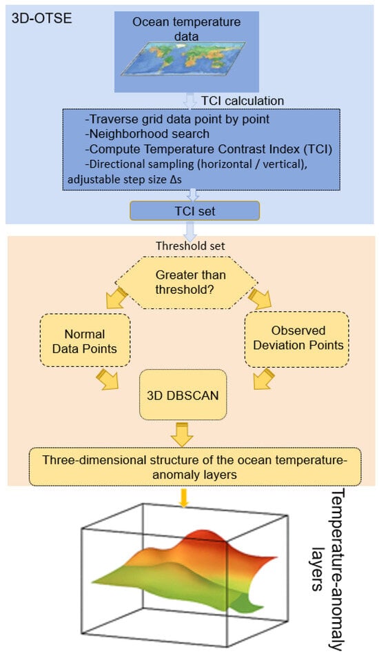
Figure 1. Flow chart of 3D-OTSE method.

Table 1. Main variables and abbreviations used in the 3D-OTSE method.

Index	Explanation
3D-OTSE	Overall framework proposed in this study for extracting 3D ocean temperature-anomaly structures.
TCI	Index that quantifies the temperature contrast between a central point and its neighborhood points.
ODP	Data points whose TCI exceeds the selected threshold and are treated as candidate anomaly members.
NDP	Data points whose TCI is less than or equal to the selected threshold and are regarded as background points.
Eps	DBSCAN parameter specifying the radius of the 3D neighborhood used to define density connectivity.
MinPts	DBSCAN parameter specifying the minimum number of points within the Eps-neighborhood required for a core point.
$N_p$	Set of neighborhood points around a given central point (default 26 points).
$d$	The i-th TCI value in the sorted TCI sequence, used as discrete sample points.
$d_i$	The i-th TCI value in the sorted TCI sequence, used as discrete sample points.
$n$	Radius of the sliding window in the polynomial fitting; each window contains 2n + 1 data points.
$a_0\dots aₘ$	Coefficients of the fitted polynomial obtained by least-squares minimization.

2.1. Calculation of the TCI

At the start of the method, this paper adopts a point-by-point traversal method, treating each point in the dataset as a central point in turn, to perform the TCI calculation for that point. As shown in Figure 2, assume the current central point is $p$, with coordinates $(x, y, z)$. A local coordinate system is established at point $p$: the z-direction is the normal direction, and $x$ and $y$ are perpendicular to $z$. In this coordinate system, a cube with $p$ as the centroid and with a side length of 2$d_{cartesian}$is constructed. The study determines that the neighborhood points set $N_p$ around point $p$ is distributed at the eight vertices and the midpoints of the twelve edges of the cube. In this coordinate system, a cube with $p$ as the centroid and with a side length of 2$d_{cartesian}$is constructed. In the default configuration used here, the neighborhood points set $N_p$ around point $p$ is distributed at the eight vertices and the midpoints of the twelve edges of the cube, yielding a 26-point vertical-oriented neighborhood that serves as a specific example of the more general parameterized scheme described below.There is a regular positional relationship between the central point $p$ and the neighborhood points set $N_p$ in the 3D coordinate system: $∆d \in \{0, d_{cartesian}, -d_{cartesian}\}$. In this coordinate system, the central point $p$ has coordinates $(x, y, z)$, and its neighborhood point set $N_p$ can be represented as:

$$N_p= \left\{\left(x+∆d,y+∆d,z+∆d\right)\right\} ∆d\in \{0,d_{cartesian},-d_{cartesian}\}$$

(1)

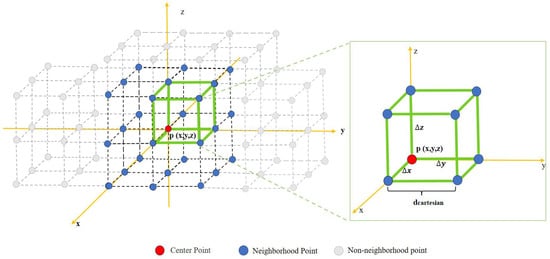
Figure 2. Position relation between center point and neighborhood point set.

To retain flexibility across different datasets and feature scales, the neighborhood $N_p$ is not restricted to a fixed 26-point configuration. In practice, we introduce a step-length parameter $\mathsf{\Delta }s$ and a directional mask that jointly control the spatial sampling pattern around the central point. When $\mathsf{\Delta }s=1$ and all three directions are activated, $N_p$ reduces to the isotropic 3 × 3 × 3 stencil used in Figure 2, containing 26 surrounding points. Increasing $\mathsf{\Delta }s$ or restricting the directional mask allows the number and orientation of neighbors to be adjusted (e.g., from a compact 26-point neighborhood to sparser stencils emphasizing only vertical columns or horizontal planes). Through this parameterization, the TCI field can be tuned to highlight different types of structures while keeping the subsequent thresholding and clustering steps unchanged. In the present study, a vertically oriented neighborhood configuration is adopted as a representative example, so that the TCI is primarily sensitive to vertical temperature transitions.

Additionally, it should be noted that for different datasets, there may be situations where the central points are located at the edges and neighborhood points are missing. For this, the method includes a verification step, which involves comparing the coordinates of the calculated neighborhood points set with the data points at the corresponding locations in the ocean temperature data to determine whether the aforementioned neighborhood points exist in the dataset. This method not only improves the performance of neighborhood point search but also ensures the accuracy of the neighborhood points set, thereby supporting the subsequent TCI calculation for each point.

TCI Calculation Method: The method for calculating TCI, based on the previously described spatial differences in point data, is as described in Equation (2) and (3):

$$K_i= {[I\left(x_i,y_i,z_i\right)-I(p_x, p_y, p_z\left)\right]}^2$$

(2)

$${TCI}_{(p_x, p_y, p_z)}={\displaystyle \frac{\sum _{i=1}^{\delta }{K}_i}{\delta }}$$

(3)

The above formula $I(p_x,p_y,p_z)$ represents the ocean temperature at the central point with coordinates $(x,y,z)$, and $I(x_i,y_i,z_i)$ represents the ocean temperature values at the coordinates of each point in the neighborhood point set $(x_i,y_i,z_i)$. $K$ represents the sum of squared differences in ocean temperature between the central point and its neighborhood points, and $\delta$ indicates the number of neighborhood points. Based on the described steps, the same calculation is performed for each point in the dataset to obtain the TCI set for all points.

2.2. Threshold Selection and ODP Screening

After completing the TCI calculations, this study moves into the threshold selection phase, aimed at accurately determining the threshold through quantitative analysis. The setting of the threshold is key to distinguishing between ODP and NDP. It requires calculation based on the distribution characteristics of the dataset or the manual setting of an appropriate threshold. The following provides a detailed introduction to the steps for selecting thresholds through calculations in more complex datasets. Considering that the dynamic environment of a large domain may exhibit spatial heterogeneity, the study area is initially divided into four subregions of equal spatial extent. The threshold-detection procedure outlined below is applied independently within each subregion, ensuring that the derived threshold accurately reflects the local statistical characteristics of the TCI field. For clarity, the following description pertains to a generic subregion; the same procedure is subsequently repeated for all subregions.

Step 1: Construction and Sorting of the TCI Sequence. For a given subregion, the TCI values of all grid points within that subregion are collected to form a local TCI set $D=\left\{TCI\right(V1),TCI(V2),...,TCI(Vn\left)\right\}$. The local TCI set is then sorted in ascending order to obtain the TCI sequence, $D_{sorted}$, for that subregion.

Step 2: Analysis of the distribution characteristics of TCI. The sorted TCI sequence $D_{sorted}$ is represented by a cumulative distribution function $F\left(d\right)$ to reveal its distribution characteristics. The cumulative distribution function $F\left(d\right)$ for the TCI in the sequence is defined as:

$$F(d)= {\displaystyle \frac{1}{n}}{\sum }_{i=1}^{n}I\left(\mathrm{T}\mathrm{C}\mathrm{I}\right(V_i)\le d)$$

(4)

Here, $I$ is the indicator function, and d is a specific TCI value. The function takes the value 1 when $TCI\left(Vi\right)\le d$, and 0 otherwise.

Step 3: Determining the Threshold. The threshold is determined by analyzing the discontinuities in the TCI distribution, which show as temperature differences between ODP and NDP. Considering that the given sequence $D_{sorted}$ is a strictly monotonically increasing sequence, the corresponding function $F\left(d\right)$ is also a monotonically increasing function. However, the forms of monotonically increasing functions are diverse, so determining a specific threshold $d_{threshold}t$ requires a thorough analysis of the trend of changes in the cumulative distribution function $F\left(d\right)$. This includes, but is not limited to, identifying critical change points in the function, such as inflection points or points of local maximum curvature, determined by the form of the function $F\left(d\right)$. The study in this section adopts a sliding window polynomial fitting method, which is described in detail as follows: Given the discrete data point set $\left\{\right(d_i,F\left(di\right)\left)\right\}$ of the cumulative distribution function $F\left(d\right)$, for each point $d_i$, a window $[d_{i-n},d_{i+n}]$ is defined, where n is the window radius. This window contains 2n + 1 data points to ensure sufficient local information for fitting. Within each window, a low-order polynomial $P\left(d\right)$is fitted to the data by the least-squares method. In this study we restrict the polynomial degree to $m\le 3$ (quadratic or cubic), in order to capture the local trend while avoiding spurious oscillations associated with higher-order fits. The polynomial has the form:

$$P\left(d\right)=a_0+a_{1}d+a_2{d}^2+\dots +a_m{d}^m$$

(5)

The objective is to minimize the error function $E$, defined as:

$$E= {\sum }_{j=i-n}^{i+n}{(F\left(d_j\right)-P\left(d_j\right))}^2$$

(6)

The polynomial coefficients $a_0,a_1$,…, am obtained by numerical methods describe the local trends and shapes of $F\left(d\right)$within the window. For each window center $d$, using the fitted polynomial $P\left(d\right)$, the curvature $\kappa$ at $d_i$ is calculated as:

$$\mathsf{\kappa }={\displaystyle \frac{\left|P^{″}\left(d_i\right)\right|}{{(1+{\left(P^{\prime }\right(d_i\left)\right)}^2)}^{\frac{3}{2}}}}$$

(7)

$P^{\prime }\left(d_i\right)$ and $P^{″}\left(d_i\right)$ are the first and second derivatives of $P\left(d\right)$ at $d_i$, respectively. For each subregion, traverse the obtained curvature values to determine the point $d_{max}$ with the maximum curvature, which is the threshold $d_{threshold}$.

The selection of ODP is based on the threshold $d_{threshold}$. Selecting points with TCI greater than the threshold from all data points, these points are identified as ODP and form the set ${\gamma }_{diff}=\left\{V_i\right|TCI\left(V_i\right)>d_{threshold},V_i\in \gamma \}$, where $\gamma$ is the set of all points. From a physical perspective, the point of maximum curvature in the cumulative TCI distribution corresponds to the transition between two distinct regimes in the vertical temperature structure of the ocean. In a stratified water column, both the mixed layer and the deep layer exhibit weak vertical temperature gradients, resulting in small and densely distributed TCI values. Conversely, subsurface temperature-anomaly layers—such as thermoclines, inversions, or other features with sharp gradients—generate large TCI values, thereby forming a sparse high-TCI tail in the distribution. The boundary between these two regimes is precisely where the cumulative distribution curve changes most abruptly, indicating the point of maximum curvature. This point marks the physical transition from weakly stratified background waters to the strong-gradient core of the thermocline (or other anomaly layers). Selecting the maximum-curvature point as the threshold effectively separates regions with physically insignificant vertical gradients from those representing meaningful temperature-gradient anomalies, thereby providing a solid physical basis for defining the ODP set.

2.3. Clustering of an ODP Set

During the selection process of the ODP set, noise or minor local variations may be included, and if these points are directly used to construct differentiation regions, errors may be introduced. To accurately extract the 3D structure of ocean temperature-anomaly layers from the ODP set, this study uses the 3D DBSCAN. This algorithm identifies and forms clusters by evaluating the local density of data points, thereby effectively distinguishing high-density areas from noise points. In the 3D formulation of DBSCAN, each ODP point is represented by its spatial coordinates $(x, y, z)$. For a given point, a three-dimensional neighborhood with a radius $\epsilon$ (Eps) is defined. If the number of neighboring points within this radius exceeds a minimum value, MinPts, the point is classified as a core point. Clusters are formed by connecting core points and their density-reachable neighbors, while isolated points that do not meet the density requirement are classified as noise. This density-based approach enables the direct identification of continuous volumetric structures from the distribution of ODPs, without imposing constraints on the geometry or smoothness of the structures. In this study, Eps and MinPts are treated as key control parameters that determine the balance between noise suppression and structural completeness. A series of parameter combinations are tested, and the clustering performance is evaluated through visual inspection and a simple clustering-effect index, aiming to minimize the influence of noise points while preserving the internal continuity of the anomaly layer. When Eps is too small or MinPts is too large, the anomaly layer may become fragmented into numerous small clusters; conversely, excessively large Eps or small MinPts may connect physically unrelated regions. The selected parameter set represents a compromise that retains the primary three-dimensional structure while filtering out isolated or weakly connected ODPs as noise. The resulting clusters produced by the 3D-DBSCAN algorithm are interpreted as three-dimensional temperature-anomaly structures, constituting the final output of the 3D-OTSE framework.

It is noteworthy that the proposed 3D-OTSE framework does not depend on regular horizontal grids or uniform sampling. The Temperature Contrast Index (TCI) is calculated solely from local vertical differences, while the 3D-DBSCAN algorithm operates directly on the existing sample points. Consequently, this method naturally accommodates sparse or irregular observational distributions, such as Argo profiles, where regions with insufficient sampling density are treated as noise according to the density-based criterion. Furthermore, the framework is applied to individual three-dimensional temperature fields, and its methodology is independent of the temporal resolution of the data. High-frequency fields capture short-term thermocline adjustments, whereas monthly or seasonal fields emphasize persistent stratification structures. The workflow itself remains unchanged, with temporal resolution affecting only the physical interpretation rather than the algorithmic steps.

3. Case Study

3.1. Study Area

This study focuses on the South China Sea (SCS) in the western Pacific. The South China Sea is one of the largest semi-enclosed seas, characterized by complex basin geometry and strong interaction with surrounding shelves and straits [30] in the world. It is adjacent to China in the north, the Indochinese Peninsula in the west, Borneo and Palawan Island in the south, and the Philippines in the east. The area of the South China Sea is about 3.5 million square kilometers. It is connected with the East China Sea through the Taiwan Strait, connected to the Pacific Ocean through the Luzon Strait, and connected to the Indian Ocean through the Sunda Strait and the Malacca Strait. The South China Sea is well-known for its complex terrain and circulation patterns. Geographically underwater, there are extensive continental shelves in the north and west, and a central deep-sea basin with a depth of more than 5000 m. Many islands and reefs (including the Xisha Islands and Nansha Islands) are scattered in the sea basin, which play a key role in the formation of regional ocean currents and mixing processes. From an oceanographic perspective, the South China Sea is affected by the East Asian monsoon system and shows obvious seasonal changes. The monsoon-driven forcing produces pronounced seasonal variations in surface circulation and upper-ocean stratification [31].The northeast monsoon generally occurs from November to March of the next year, bringing cool and dry air and making the ocean surface water flow southward. In turn, the southwest monsoon lasts from May to September, producing northward or eastward flow and enhancing water column stratification. The characteristic of the monsoon transition period is the change in wind direction and ocean circulation, forming a dynamic thermohaline structure. In addition, the South China Sea is connected with adjacent ocean basins through major straits and channels, promoting a large amount of water exchange with the Pacific Ocean and the Indian Ocean. Mesoscale eddies also play a significant role in redistributing heat and modifying the vertical temperature structure across different seasons [27].These exchanges, plus the influence of monsoons and terrain restrictions, make the South China Sea an excellent natural place for studying ocean phenomena such as thermocline dynamics, vertical mixing, and mesoscale changes. The depth and intensity of the seasonal thermocline in the region exhibit significant spatial variability due to the combined influence of circulation and mixing processes.

This study conducts an investigation on the entire South China Sea, covering the range of approximately 5–23° north latitude and 105–121° east longitude. This area includes the continental slope and shelf areas on the northern and western margins, and the central deep-sea basin of the South China Sea, as shown in Figure 3. Such a vast geographical range allows in-depth research on hydrological characteristics, circulation dynamics, and various processes in the main seas of the South China Sea.

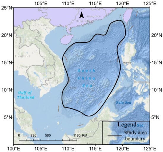
Figure 3. Study area of the South China Sea.

Previous observational and modeling studies have consistently demonstrated that the deep basin of the South China Sea features a pronounced and persistent seasonal thermocline. Based on SODA reanalysis and historical hydrographic profiles, Pan et al. (2018) reported that in the region approximately between 5 and 23° N and 105–121° E, the upper boundary of the thermocline typically occurs at depths of 40–80 m, while the lower boundary remains between approximately 150–250 m, exhibiting only modest seasonal variations [27]. Analyses of hydrographic sections and moored temperature records by Liu et al. (2000, 2001) further revealed a strong vertical temperature gradient within this depth range across the deep central basin, underscoring a robust and recurrent thermocline structure that dominates upper-ocean stratification [28,32]. Lan et al. (2006) demonstrated that monsoon-driven circulation and basin-scale ocean dynamics exert significant control over the spatial continuity and large-scale tilt of this thermocline [33]. Furthermore, Hao et al. (2012) confirmed—through gradient-based diagnostics applied to the China Seas and the northwestern Pacific—that the South China Sea contains one of the most stable and spatially coherent seasonal thermoclines in the region [31].

These previous studies indicate that the study region analyzed in this work is a well-established thermocline-dominated environment, providing a physically consistent framework for interpreting the extracted temperature-anomaly structure in subsequent sections.

3.2. Data

The experimental data utilized in this study comprise the monthly mean temperature field for April 2020 obtained from the GDCSM_Argo global dataset. This dataset has been refined to concentrate on the South China Sea region, where the upper-ocean thermal structure and the thermocline depth are known to exhibit significant spatial and temporal variability [27,32]. The dataset provides three-dimensional temperature fields on a horizontal grid of 1° × 1°, with 57 vertical layers extending from the surface to a depth of 2000 m [34]. This resolution is adequate to capture the main thermocline and deeper stratification within the basin [35]. The South China Sea subset utilized in this study is illustrated in Figure 4, which clearly delineates the vertical transitions in temperature structure across various depth levels.

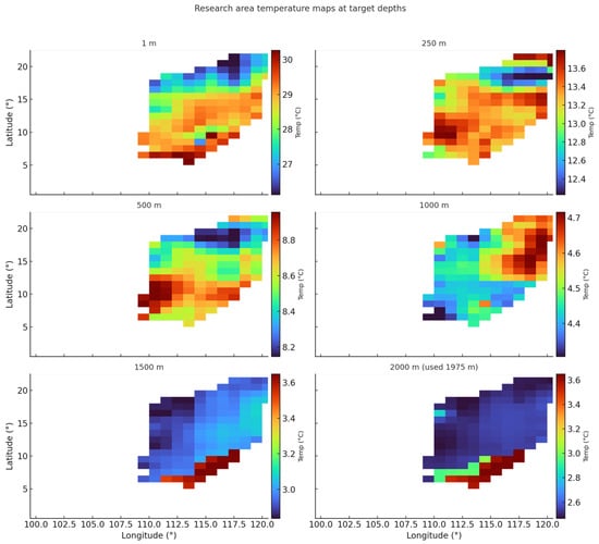
Figure 4. The monthly average temperature profile distribution in the South China Sea for April 2020, with a spatial resolution of 1° × 1°. The overall model temperature exhibits a characteristic pattern of lower temperatures in the northern region and higher temperatures in the southern region above a depth of 500 m. Below 500 m, temperatures are generally lower, with relatively lower temperatures observed in the southern region.

4. Results

In the following, the 3D-OTSE framework is applied to the South China Sea. We adopt the vertically oriented neighborhood configuration described in Section 2.1, ensuring that the TCI primarily reflects vertical temperature contrasts associated with thermocline structures. All results presented in this section are derived from this parameter setting, representing a specific realization of the general parameterized scheme.

4.1. Threshold Setting

By calculating the TCI of the GDCSM_Argo global ocean temperature data, a TCI sequence $D=\left\{TCI\right(V1),TCI(V2),\dots ,TCI(Vn\left)\right\}$ is constructed. The sequence is numerically sorted to obtain $D_{sorted}$, and the cumulative distribution function $F\left(d\right)$ is calculated based on $D_{sorted}$. Since the dynamical environment within the study area is not spatially homogeneous, the threshold detection is performed independently within each of the four subregions defined in Section 2.2. The threshold illustrated here represents the process applied to one subregion, as the same procedure is identical for all subregions. The regional thresholds are then combined through the ODP-merging step to obtain the final ODP field used for 3D reconstruction. As shown in Figure 5, the cumulative distribution function $F\left(d\right)$ is a monotonically increasing convex function, and its threshold should be the point of local maximum curvature of the function. The local maximum curvature point $d_{max}$ = 0.32 is determined by the sliding window polynomial fitting method mentioned in Section 2.3, and the threshold $d_{threshold}$ is thus obtained as 0.32.

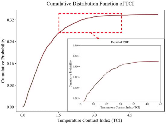
Figure 5. The cumulative distribution function of the TCI.

In the 3D DBSCAN stage, the experiment set Eps to 2, 3, 4, and 5, respectively, to select overlapping areas. For handling noise and smaller clustered areas, the experiment set the MinPts to 10 to eliminate noise; clustered areas were sorted by the number of points, and areas with more points were taken as the final result, with smaller areas excluded from the study.

4.2. Three-Dimensional Anomaly Layer Structure Extraction

This study explores the South China Sea by analyzing Argo profiles obtained through the proposed TCI-threshold-3D clustering method. The ODP field utilized for reconstruction incorporates regionally adaptive thresholds, ensuring that spatial variations in stratification intensity across the South China Sea are accurately represented. With the ODP field established for each subregion, the spatial organization of the primary subsurface temperature-transition feature can be analyzed. By aggregating ODP into coherent volumetric clusters, the adaptive 3D-OTSE framework elucidates the dominant temperature-contrast layer embedded within the April 2020 South China Sea temperature field. The depth distributions of the upper and lower interfaces of this layer, illustrated in Figure 6a,b, are derived solely from data-driven thresholding and clustering, devoid of any thermocline-specific assumptions.

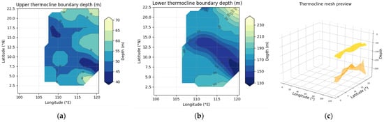
Figure 6. Data-driven temperature-anomaly structure extracted by the 3D-OTSE framework. (a) Plan-view depth of the upper boundary of the detected temperature-contrast layer. (b) Plan-view depth of the lower boundary. (c) Three-dimensional mesh of the upper and lower interfaces illustrating the volumetric geometry of the dominant temperature-anomaly layer present in the dataset. Note that 3D-OTSE does not assume a thermocline; the thermocline-like pattern shown here arises from the dataset itself.

In this dataset, the extracted anomaly layer naturally assumes a thermo-cline-like form. The upper interface remains relatively shallow, primarily ranging from 45 to 60 m, while the lower interface exhibits a pronounced deepening from the southwestern basin (approximately 150 to 180 m) toward the northeastern deep-water region (exceeding 220 m). This west-to-east deepening results in a progressively thickening transition layer, aligning with the large-scale stratification pattern characteristic of the South China Sea. Importantly, this structure is not dictated by the method; rather, it arises as the most coherent temperature-gradient feature present in the underlying field. A three-dimensional visualization of the extracted boundaries (Figure 6c) underscores the continuity and volumetric geometry of this temperature-anomaly layer. The reconstructed surfaces create a smooth yet undulating three-dimensional structure, exhibiting basin-scale tilting and localized domes and depressions likely linked to mesoscale variability. These features demonstrate that the flexible, parameter-adaptive design of 3D-OTSE effectively mitigates noise while maintaining the essential three-dimensional morphology of the detected anomaly layer—whether it resembles a thermocline, an inversion, or another type of subsurface transition.

To further clarify the internal organization of the data-driven temperature-transition layer identified by 3D-OTSE, we supplement the plan-view and interface-based description of Figure 6 with a longitudinal cross-section and volumetric reconstruction of the extracted structure (Figure 7). While Figure 6 highlights the horizontal geometry of the upper and lower interfaces, the cross-sectional view in Figure 7a reveals how these interfaces enclose a coherent subsurface band when examined in the depth-latitude plane. Along the representative meridional section, the region situated between the two OTSE-derived boundaries forms a continuous, well-defined anomaly band, despite considerable spatial variations in its depth and thickness. Observations show that the boundaries clustered by the local ODP are not just patches connecting isolated strong temperature contrasts; they represent a volume-consistent transition layer in the vertical stratification of the South China Sea. The morphology inside the anomaly zone provides clues for understanding the three-dimensional structure of the transition layer. In the southern part of the section, this layer is relatively thin and shallow, reflecting the weak vertical stratification in the low-latitude area and the dominance of warm surface water. Moving northward, the thickness of this zone obviously increases, and the depth of the lower interface is greatly deepened. This observation result is consistent with the basin-scale tilt in Figure 6. The lower bound is thickened and displaced downward, the temperature-contrast layer is asymmetric, and it is adapted to the vertical shear of temperature in the subtropical South China Sea. It should be noted that this behavior originates from local adaptive threshold processing and ODP clustering, not from the prior assumption of a similar thermocline structure. The 3D rendering in Figure 7b places the cross-section interpolation in the basin space background. From the perspective of the volume entity, the abnormal layer has a smooth upper surface modulated by mesoscale wave-like structures, and the lower surface is mostly explained as vertical changes, making the main body thicken in the deep basin in the northeast. The continuous 3D volume confirms that the adaptive 3D-OTSE framework can capture the transition layer. Although there are mesoscale changes and vertical complexity in the temperature field, the transition layer can still extend throughout the region. The congruence between the meridional section and the 3D structure further illustrates that the extracted layer represents a basin-scale temperature-contrast feature inherent to the data and verifies that this method can find the ability of flexible, non-parametric analogs such as thermocline anomalies without determining the geometric shape or depth range in advance.

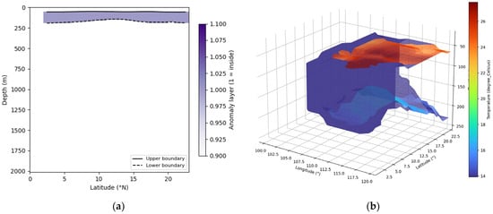
Figure 7. (a) Meridional section of the 3D-OTSE-extracted anomalous layer along about 115°E. The shaded areas mark the data-driven upper bound (solid line) and lower bound (dashed line), showing that the detected structure is a continuous subsurface zone, not isolated patches. (b) 3D rendering of the same anomaly, colored according to in situ temperature for enhanced visibility. This structure is coherent throughout the basin, deepening/thickening towards the northeast, consistent with the spatial variation in Figure 6.

Shift from basin scale to fine abnormal structure. As shown in Figure 8, intralayer organic groups are locally observed. Within the extracted range, the anomaly has a smooth surface, and the curvature of this surface is relatively gentle, which is associated with small undulations and medium-scale variables. By modulating the temperature field, since it is not the extraction process, this method retains the inherent structure of the transition zone without being too smooth. The vertical section again clarifies the temperature groups. The isotherms converge/bend towards the anomaly center, forming a vertically coherent transition zone with the strongest gradient. Near the abnormal boundary, the vertical gradient decreases and the width become wider, indicating that its structure is not a single sharp interface, but a multi-layer transition zone with a core area and flank belts. This pattern persists along the section, highlighting that the anomaly is a spatially coherent subsurface feature, and the internal layers remain unchanged at long distances. In conclusion, these features show that the 3D-OTSE framework not only depicts the geometric form of the main temperature transition anomaly but also retains the internal thermal structure. The extracted layer segments have physically understandable gradient cores, spatially variable internal curvatures, and cross-basin coherent connections, supplementing the earlier more extensive tectonic features.

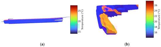
Figure 8. Extracts the detailed internal structure of the temperature-transition anomaly. (a) The 3D-OTSE obtains a smooth internal geometry and a local 3D view with fine undulations. (b) The vertical temperature profile of the same feature shows the convergence of abnormal isotherms and the formation of a coherent internal transition zone.

At several depths to check the temperature field in the horizontal direction (Figure 9), to have a broader understanding of the environment around the extracted anomaly. These depth slices show the vertical evolution of the environmental thermal structure and how the lateral changes provide the background for the three-dimensional anomaly. At a depth of 50 m, there is a warm water body in the temperature field, accompanied by obvious lateral gradients, filamentous warm spots, and irregular cold intrusions. These patterns show that they are obviously modulated by mesoscale and submesoscale processes, indicating that the upper-layer transport environment is partially far from the state of horizontal uniformity. At a depth of 100 m, the spatial pattern is more inhomogeneous: warm/cold areas are interlaced in the basin, and the gradients are more fragmented and segmented. This depth initiates a broader transition state. In this state, the surface-modified water interacts with the relatively cold water at the middle depth. The irregularity of this layer field implies that the coherent subsurface structure within this range originates from the collective organization of spatial contrast, not a simple monotonous vertical profile. A more distinct transition environment can be seen at 150 m, where the temperature drops sharply. At this depth, the horizontal gradient creates coherent cold features spanning tens to hundreds of kilometers. These colder anomalies mix with the warm water tongues coming from adjacent areas, forming a complex middle-depth thermal mosaic. This depth is in the core of the vertical evolution transition zone, with strong lateral changes and changes in local layered structures. The extracted anomaly matches this depth range because the temperature contrast defining the structure is most obvious here. When reaching 200 m, the temperature field is colder and more uniform. The weakening of the lateral gradient at this depth and the contrast with the variability above mark the transition to a weakly stratified deep layer. The reduction in the horizontal structure from 50 m to 200 m outlines the situation where the anomaly is embedded in the vertical background, which indicates that the extracted geometric shape reflects the inherent organization of the temperature field. The changes at different depth multi-scale levels, the 3D anomalies reconstructed by 3D-OTSE, which originate from the spatial coherent patterns inherent in the data, not from the rigidly added structural assumptions.

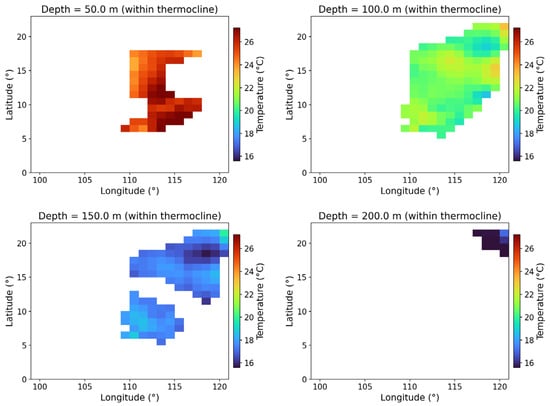
Figure 9. Horizontal temperature fields at 50, 100, 150, and 200 m, illustrating the depth-dependent lateral variability of the ambient thermal environment. The upper layers exhibit warm patches and strong mesoscale modulation, while the mid-depth fields show sharper horizontal contrasts and the coexistence of multiple thermal regimes. The deeper layer becomes more uniform and markedly cooler. These depth slices provide background context for the three-dimensional transition anomaly extracted by 3D-OTSE, showing the spatial patterns from which the volumetric structure emerges.

5. Discussion

The central contribution of 3D-OTSE is that it reframes the problem from estimating a specific type of boundary to identifying coherent temperature-anomaly structures directly from the full three-dimensional field. Many subsurface features of interest—including inversion layers, multilayer transition zones, and eddy-induced subsurface anomalies—do not conform to the monotonic vertical patterns assumed by classical profile-based diagnostics. Because those methods evaluate each cast independently, they cannot determine whether locally detected transitions belong to the same spatially coherent structure. By combining an adaptive TCI threshold with three-dimensional clustering, 3D-OTSE extracts volumetric anomalies in a fully data-driven manner without prescribing their shape, physical interpretation, or depth range in advance. This general formulation enables the method to reveal whichever transition structure is actually present in the data, providing a capability that traditional two-dimensional diagnostics lack. Compared with traditional two-dimensional profile-based schemes for detecting mixed-layer or thermocline boundaries [10], the proposed 3D-OTSE framework shows clear advantages in spatial completeness, structural continuity, and robustness to sampling irregularities. By defining a three-dimensional temperature-contrast index and combining it with density-based clustering [29], the method extracts coherent volumetric temperature-anomaly structures rather than inferring interfaces from isolated vertical profiles.

The 3D abnormal layer reconstructed above the South China Sea reflects the basin-scale air–sea interaction and regional circulation. The vertical displacement of isotherms caused by seasonal monsoons, and interannual modes such as ENSO will change the stratification and heat content of the upper ocean [31,32]. The intrusion of the Kuroshio, mesoscale eddies, and the increase in internal waves enhance the lateral inhomogeneity, making the subsurface temperature state have dynamic coupling and spatially complex characteristics.

In order to clarify its connection with the conventional diagnostic method, as shown in Figure 10,the boundary based on 3D-OTSE will be compared with the boundaries obtained by the S-type vertical gradient method by Romero et al. (2023) [13] and the S-type fitting method based on the zero vertical gradient criterion. The temperature gradient is 0.5 °C/m. The deep sea basin shows a uniformly stratified state, and the depth ranges involved in each method are similar to each other, which is consistent with the previous observation of the thermocline [27]. In the nearshore shelf break area, there are internal wave breaking, tidal mixing, freshwater input, and topographic guidance to reshape the vertical gradient, and the differences are obvious [32]. The gradient method shows the most obvious changes in each profile, and 3D-OTSE captures the horizontal coherent patterns of the 3D field. The three methods capture different aspects of the thermal structure. This difference should exist originally and has scientific significance. The near-shore transition zone is very active and has high biological productivity [25].

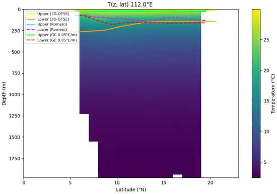
Figure 10. Comparison of subsurface boundary estimates obtained using the 3D-OTSE framework and the sigmoidal vertical-gradient method of Romero et al. (2023) [13] and a vertical-gradient criterion (0.05 °C m⁻¹). The deep-basin thermocline depths are generally comparable between the three approaches, while coastal and shelf-break regions exhibit marked discrepancies associated with spatially heterogeneous stratification and mixing processes.

Although there are many differences, the large-scale thermocline-like structure made by 3D-OTSE is very consistent with the existing regional models. The regional adaptive threshold makes it reliable for each sub-region to adjust its own specific stratification state. The traditional gradient method can give clear local diagnosis, and 3D-OTSE can highlight spatial coherence; the combination of the two can have a more comprehensive understanding of the upper-layer ocean thermal structure.

There are obvious limitations. The accuracy of reconstructing the 3D structure depends on the resolution and smoothness of the data; monthly fields may mask fine changes. If the threshold is selected too large, it will affect the sensitivity to noise, and DBSCAN parameters will also affect clustering. When applying this method to other river basins or multivariate data, relevant dynamic characteristics need to be considered. Future improvements may include underground reconstruction based on machine learning and cutting-edge detection techniques [19] to improve the generality of the method. The 3D-OTSE framework coordinates 3D anomaly extraction and traditional profile diagnosis methods and is a flexible data-driven tool for reconstructing subsurface structures from multi-depth ocean temperature fields. Case studies in the South China Sea show that this method can effectively reproduce layers with complex geometries similar to well-documented thermoclines. Future research may include time-evolving datasets and additional variables (such as density, salinity, and biogeochemical tracers) to study how different ocean anomaly layers interact with circulation, climate variables, and ecosystem responses.

6. Conclusions

The 3D-OTSE described in this study is a data-driven framework. It is used to extract 3D subsurface structures from multi-depth ocean temperature fields. Combined with the volume temperature contrast index and density-based clustering, this method can find coherent temperature transition layers without relying on strong prior assumptions in traditional profile diagnostics. When applied to the South China Sea, 3D-OTSE reproduces features similar to the thermocline and mesoscale patterns, providing a comprehensive 3D perspective for traditional gradient applications. In the current implementation, taking the vertical neighborhood configuration as an example, it is ensured that the temperature contrast index is mainly sensitive to vertical changes related to the thermocline structure. However, the neighborhood of 3D-OTSE is parameterized by adjustable step size ranges and direction masks, enabling flexible reconfiguration of sampling patterns. For example, emphasize vertical columns, horizontal planes, or multi-scale templates to adapt to different marine regions or observation research objectives. This flexible approach enables the framework to be adjusted without changing the overall process to adapt to other variables and observation requirements, thus laying the foundation for future development, such as time-dependent data or integrating temperature, density, salinity, and biogeochemical tracers to further figure out the dynamics of oceanic anomalous layers.

References

- Roemmich, D.; Gilson, J. The 2004–2008 mean and annual cycle of temperature, salinity, and steric height in the global ocean from the Argo Program. Prog. Oceanogr. 2009, 82, 81–100. [Google Scholar] [CrossRef]
- Cheng, L.; Abraham, J.; Hausfather, Z.; Trenberth, K.E. How fast are the oceans warming? Science 2019, 363, 128–129. [Google Scholar] [CrossRef]
- Chelton, D.B.; Schlax, M.G.; Samelson, R.M. Global observations of nonlinear mesoscale eddies. Prog. Oceanogr. 2011, 91, 167–216. [Google Scholar] [CrossRef]
- Zhang, Z.; Wang, G.; Wang, H.; Liu, H. Three-dimensional structure of oceanic mesoscale eddies. Ocean-Land-Atmos. Res. 2024, 3, 0051. [Google Scholar] [CrossRef]
- Zhuang, Z.; Zhang, Y.; Zhang, L.; Ruan, W.; Lyu, D.; Yu, J. Reconstructing the three-dimensional thermohaline structure of mesoscale eddies in the South China Sea using in situ measurements and multi-sensor satellites. Remote Sens. 2024, 17, 22. [Google Scholar] [CrossRef]
- Cruz, N.A.; Matos, A.C. Reactive AUV motion for thermocline tracking. In Proceedings of the Oceans 10 IEEE Sydney, Sydney, Australia, 24–27 May 2010; pp. 1–6. [Google Scholar]
- Zhang, Y.; Bellingham, J.G.; Godin, M.A.; Ryan, J.P. Using an autonomous underwater vehicle to track the thermocline based on peak-gradient detection. IEEE J. Ocean. Eng. 2012, 37, 544–553. [Google Scholar] [CrossRef]
- Ker, S.; Le Gonidec, Y.; Marie, L.; Thomas, Y.; Gibert, D. Multiscale seismic reflectivity of shallow thermoclines. J. Geophys. Res. Ocean. 2015, 120, 1872–1886. [Google Scholar] [CrossRef]
- Chu, P.C.; Fan, C. Determination of Ocean Mixed Layer Depth from Profile Data. In Proceedings of the 15th Symposium on Integrated Observing and Assimilation Systems for the Atmosphere, Oceans and Land Surface (IOAS-AOLS), Seattle, WA, USA, 23–27 January 2011; pp. 1001–1008. [Google Scholar]
- Kara, A.B.; Rochford, P.A.; Hurlburt, H.E. An optimal definition for ocean mixed layer depth. J. Geophys. Res. Ocean. 2000, 105, 16803–16821. [Google Scholar] [CrossRef]
- de Boyer Montégut, C.; Madec, G.; Fischer, A.S.; Lazar, A.; Iudicone, D. Mixed layer depth over the global ocean: An examination of profile data and a profile-based climatology. J. Geophys. Res. Ocean. 2004, 109, C12003. [Google Scholar] [CrossRef]
- Tang, H.; Wang, C.; Li, H.; He, Y. Ocean mixed layer depth 2000–2020: Estimation assessment and long-term trends. Prog. Oceanogr. 2025, 234, 103467. [Google Scholar] [CrossRef]
- Romero, E.; Tenorio-Fernandez, L.; Portela, E.; Montes-Aréchiga, J.; Sánchez-Velasco, L. Improving the thermocline calculation over the global ocean. Ocean. Sci. 2023, 19, 887–901. [Google Scholar] [CrossRef]
- Ji, X.; Feng, M.; Wang, J. Characterization of the thermocline in the eastern Pacific Ocean based on a hyperbolic tangent function fitting method. Ocean. Dyn. 2025, 75, 81. [Google Scholar] [CrossRef]
- Belkin, I.M.; O’Reilly, J.E. An algorithm for oceanic front detection in chlorophyll and SST satellite imagery. J. Mar. Syst. 2009, 78, 319–326. [Google Scholar] [CrossRef]
- Xing, Q.; Yu, H.; Yu, W.; Chen, X.; Wang, H. A global daily mesoscale front dataset from satellite observations: In situ validation and cross-dataset comparison. Earth Syst. Sci. Data 2025, 17, 2831–2848. [Google Scholar] [CrossRef]
- Xing, Q.; Yu, H.; Wang, H.; Ito, S.I. An improved algorithm for detecting mesoscale ocean fronts from satellite observations: Detailed mapping of persistent fronts around the China Seas and their long-term trends. Remote Sens. Environ. 2023, 294, 113627. [Google Scholar] [CrossRef]
- Kong, R.; Liu, Z.; Wu, Y.; Fang, Y.; Kong, Y. Intelligent Detection of Oceanic Front in Offshore China Using EEFD-Net with Remote Sensing Data. J. Mar. Sci. Eng. 2025, 13, 618. [Google Scholar] [CrossRef]
- Su, H.; Wang, A.; Zhang, T.; Qin, T.; Du, X.; Yan, X.H. Super-resolution of subsurface temperature field from remote sensing observations based on machine learning. Int. J. Appl. Earth Obs. Geoinf. 2021, 102, 102440. [Google Scholar] [CrossRef]
- Zhang, J.; Zhang, X.; Wang, X.; Ning, P.; Zhang, A. Reconstructing 3D ocean subsurface salinity (OSS) from T–S mapping via a data-driven deep learning model. Ocean. Model. 2023, 184, 102232. [Google Scholar] [CrossRef]
- Qi, J.; Liu, C.; Chi, J.; Li, D.; Gao, L.; Yin, B. An ensemble-based machine learning model for estimation of subsurface thermal structure in the South China Sea. Remote Sens. 2022, 14, 3207. [Google Scholar] [CrossRef]
- Yu, X.; Yi, D.L.; Wang, P. Enhancing Ocean Temperature and Salinity Reconstruction with Deep Learning: The Role of Surface Waves. J. Mar. Sci. Eng. 2025, 13, 910. [Google Scholar] [CrossRef]
- Luo, C.; Huang, M.; Guan, S.; Zhao, W.; Tian, F.; Yang, Y. Subsurface Temperature and Salinity Structures Inversion Using a Stacking-Based Fusion Model from Satellite Observations in the South China Sea. Adv. Atmos. Sci. 2025, 42, 204–220. [Google Scholar] [CrossRef]
- Wang, Q.; Zhang, X.; Wu, X.; Zhang, D.; Qi, J.; Ning, P.; Qiao, X. Deep Learning–based Eddy-resolving Reconstruction of Subsurface Temperature and Salinity in the South China Sea. Adv. Atmos. Sci. 2025, 42, 1675–1692. [Google Scholar] [CrossRef]
- Cantin, A.; Beisner, B.E.; Gunn, J.M.; Prairie, Y.T.; Winter, J.G. Effects of thermocline deepening on lake plankton communities. Can. J. Fish. Aquat. Sci. 2011, 68, 260–276. [Google Scholar] [CrossRef]
- Holte, J.; Talley, L. A new algorithm for finding mixed layer depths with applications to Argo data and Subantarctic Mode Water formation. J. Atmos. Ocean. Technol. 2009, 26, 1920–1939. [Google Scholar] [CrossRef]
- Peng, H.; Pan, A.; Zheng, Q.A.; Hu, J. Analysis of monthly variability of thermocline in the South China Sea. J. Oceanol. Limnol. 2018, 36, 205–215. [Google Scholar] [CrossRef]
- Liu, Q.; Yang, H.; Qi, W. Dynamic characteristics of seasonal thermocline in the deep sea region of the South China Sea. Chin. J. Oceanol. Limnol. 2000, 18, 104–109. [Google Scholar] [CrossRef]
- Chen, H.; Liang, M.; Liu, W.; Wang, W.; Liu, P.X. An approach to boundary detection for 3D point clouds based on DBSCAN clustering. Pattern Recognit. 2022, 124, 108431. [Google Scholar] [CrossRef]
- Qu, T. Upper layer circulation in the South China Sea. J. Phys. Oceanogr. 2000, 30, 1450–1460. [Google Scholar] [CrossRef]
- Hao, J.; Chen, Y.; Wang, F.; Lin, P. Seasonal thermocline in the China Seas and northwestern Pacific Ocean. J. Geophys. Res. Ocean. 2012, 117, C02022. [Google Scholar] [CrossRef]
- Liu, Q.; Jia, Y.; Liu, P.; Wang, Q.; Chu, P.C. Seasonal and intraseasonal thermocline variability in the central South China Sea. Geophys. Res. Lett. 2001, 28, 4467–4470. [Google Scholar] [CrossRef]
- Lan, J.; Bao, Y.; Yu, F. Seasonal variabilities of the circulation and thermocline depth in the South China Sea deep water basin. Adv. Mar. Sci. 2006, 24, 436. [Google Scholar]
- Xie, C.; Xv, M.; Cao, S.; Zhang, Y.; Zhang, C. Gridded Argo data set based on GDCSM analysis technique: Establishment and preliminary applications. J. Mar. Sci. 2019, 37, 24–35. [Google Scholar]
- Peng, H.; Pan, A.; Zheng, Q.A.; Hu, J. A study of response of thermocline in the South China Sea to ENSO events. J. Oceanol. Limnol. 2018, 36, 1166–1177. [Google Scholar] [CrossRef]
Disclaimer/Publisher’s Note: The statements, opinions and data contained in all publications are solely those of the individual author(s) and contributor(s) and not of MDPI and/or the editor(s). MDPI and/or the editor(s) disclaim responsibility for any injury to people or property resulting from any ideas, methods, instructions or products referred to in the content. |
© 2025 by the authors. Licensee MDPI, Basel, Switzerland. This article is an open access article distributed under the terms and conditions of the Creative Commons Attribution (CC BY) license (https://creativecommons.org/licenses/by/4.0/).