Impact of Fluid Sloshing on BOG Generation in Type B LNG Tanks During Ship Emergency Stops

Abstract

The safe and efficient transport of Liquefied Natural Gas (LNG) is critically dependent on understanding fluid dynamics within cargo tanks, which directly influence structural integrity and operational safety. Study employs the Volume of Fluid (VOF) method to simulate fluid sloshing and phase change dynamics in Type B LNG cargo tanks during emergency stop conditions. The transient simulations employ a time step of 5 × 10⁻³ s, a model with 46,840 grids, and the analysis focuses on impact forces on tank walls, their dependence on filling levels. Results show that the flow disturbance caused by vessel rolling increases BOG generation fluctuations by approximately 35%. Sloshing significantly increases BOG generation, particularly after a 10 s relaxation period, as the initial shock enhances heat transfer and mixing, accelerating vapor production. Original components of LNG are sensitive to BOG generation and impact forces on the front bulkhead are significantly higher than on the rear, with peak impacts occurring. The filling rate is a critical parameter influencing fluid dynamics and safety in LNG transportation. Impact magnitude increases with fill level up while at about 80% it declines; impact timing shortens at higher fill ratios. A BOG generation mechanism in which microscale turbulence and ongoing thermal imbalance govern the kinetics of evaporation phase transitions was proposed. It was discovered that the impact forces and BOG production exhibit rise–fall–rise patterns driven by impact dynamics, condensation, and evaporation processes. The findings highlight the critical role of fluid sloshing in affecting tank safety and operational efficiency, offering insights into designing more resilient LNG cargo tanks and optimizing transportation safety and economy.

1. Introduction

Natural gas (NG) remains a vital energy resource due to its extensive reserves and widespread utilization worldwide. Over the past century, from 1920 to 2021, global natural gas production increased by more than 150 times, from 2.28 × 10⁹ m³ to 4.04 × 10¹² m³. Currently, NG accounts for approximately 24.72% of the world’s energy consumption, underscoring its significant role in global energy systems [1]. Among the transportation methods, liquefied natural gas (LNG) shipping is the most crucial for cross-border maritime trade, primarily facilitated through specialized LNG carriers. During transportation, a temperature difference of approximately 190 K exists between the LNG and the surrounding environment [2]. Despite insulation measures, external heat ingress causes continuous vaporization within the cargo hold. This process is further intensified by fluid sloshing induced by vessel motion, which inevitably leads to the formation of Boil-Off Gas (BOG). The mechanisms by which fluid sloshing influences BOG generation, along with effective control measures, represent a critical scientific and engineering challenge. Addressing this issue is vital, as it directly affects operational safety, economic efficiency, and overall system performance during LNG transportation. Ship sway (including roll, pitch, and heeling) can substantially amplify BOG generation, with increases ranging from 1.5 to over 4 times the baseline static BOG rate. Excessive BOG risks pressure buildup and leaks and understanding BOG trends enables better control strategies. Optimizing venting and reliquefication systems ensures safety, system stability, and cost-effectiveness. Particularly, understanding the impact of fluid sloshing on BOG generation rates and developing effective control strategies are essential steps toward improving safety and optimizing operational efficiency in LNG transit.

Fluid sloshing within cargo tanks is characterized by strongly nonlinear motion. When the free surface impacts the tank walls, it exerts significant impact forces, which can threaten structural integrity. Research on fluid sloshing phenomena in cargo tanks has primarily relied on three methodological approaches: theoretical analysis, which provides fundamental insights into the underlying physics; numerical simulation, enabling detailed modeling of complex sloshing behaviors; and experimental testing, offering empirical validation of theoretical and computational results. Theoretical methods, however, often face limitations in effectively capturing and resolving practical problems due to inherent simplifications. Experimental research provides the most direct insights into sloshing phenomena. Moreover, numerous scholars have carried out experimental investigations into sloshing loads, yet such methods demand substantial human and material resources and are typically confined to limited environmental conditions. Recent advances in computational technology have significantly enhanced the role of numerical simulations. Muttaqie et al. [3] employed finite element analysis to study the structural strength of designed LNG cargo tanks. Similarly, Chong W et al. [4] utilized the Volume of Fluid (VOF) method to simulate LNG filling processes under sloshing conditions, analyzing disturbance variations in different stratified states. Lee et al. [5] applied computational fluid dynamics (CFD) techniques to simulate sloshing in LNG tanks, focusing on impact forces exerted on tank walls. Additionally, Miana et al. [6] assessed heat transfer from the environment to LNG on a Mark III type transport vessel, providing insights into thermal effects during transportation. These studies have collectively established a foundation for further exploration of fluid sloshing in LNG cargo tanks.

Developing advanced LNG tank models based on computational fluid dynamics (CFD) is essential for accurately predicting fluid flow behavior and Boil-Off Gas (BOG) generation, thereby deepening the understanding of LNG tank performance. Lin et al. [6] proposed a novel equivalent conduction model, replacing traditional multiphase flow approaches to simulate BOG mass and flow dynamics more efficiently. Zakaria et al. [7,8,9,10] employed ANSYS Fluent (2025R1) to simulate full-scale LNG ships, enabling the estimation of BOG generation within cargo holds. Similarly, Niu et al. [11] utilized ANSYS Fluent to develop a heat transfer model for an independent B-type LNG carrier, allowing precise determination of temperature fields and BOG rates under various operating conditions. Complementary to these studies, numerical simulations of heat transfer and phase change phenomena in cryogenic systems, combined with investigations into LNG tank aging and BOG evolution under different operational scenarios, provide critical insights into LNG behavior during storage and transportation. Jeon et al. [12] applied CFD techniques to analyze heat transfer and phase change processes within cryogenic tank insulation systems, revealing complex phenomena such as natural convection and phase transition effects that are difficult to capture through experiments. Ferrin et al. [13] constructed a heat transfer model for small LNG pressure vessels using ANSYS Fluent, quantifying heat loss and evaporation rates with respect to insulation layer thickness and filling rate; their results indicated that, at low filling levels, the liquid tends toward an approximate isothermal state. Recent efforts have shifted toward multi-zone thermodynamic modeling to better assess aging effects in LNG storage tanks. Chen et al. [14] proposed a multi-region model, observing that increased methane concentration initially reduced the BOG rate, although this sensitivity diminished over time. Jung et al. [15] developed a model simulating tank aging under isobaric conditions, solving coupled heat and mass transfer equations to validate the model against experimental data. Duan et al. [16] derived the integral form of buoyancy-driven flow equations, elucidating the evolution of thermal phenomena such as steam superheating during evaporation processes. The magnitude of ship motion, particularly sloshing amplitude, and the filling rate of LNG tanks are critical parameters influencing the fluid dynamics and safety during LNG transport. Additionally, Increased sloshing amplitude can intensify pressure fluctuations and fluid–structure interactions, potentially amplifying BOG generation and impacting structural integrity [16]. Similarly, the filling rate affects the free surface level and sloshing intensity, directly correlating with pressure oscillations and phase-change phenomena [13]. Understanding these parameters’ roles is essential for accurate modeling and designing effective control strategies. Precise quantification and simulation of their impacts enable better prediction of transient behaviors, ultimately enhancing safety and operational reliability in LNG shipping.

Type B LNG tanks are highly reliable, based on precise calculations, and do not solely rely on primary barriers. They are ideal for high-safety applications, harsh routes like the Arctic, and flexible operations, making them the preferred choice for extreme conditions. However, developing a fully coupled thermodynamic–hydrodynamic model for LNG tanks that accurately reflects actual ship motion conditions remains a highly challenging task. This endeavor necessitates a comprehensive understanding of cryogenic liquid sloshing behaviors and heat transfer mechanisms under dynamic environments. Furthermore, it requires the precise extraction and analysis of sloshing-induced thermodynamic variations, which are also critical for informing structural optimization and enhancing the safety of LNG containment systems. Addressing these complexities is essential to improve the reliability and operational safety of LNG storage during marine transit. Refs. [17,18] emphasize variations in the gas–liquid interface and pressure loads induced by sloshing; however, the effects of heat transfer on these processes are insufficiently addressed [19,20,21]. There are studies that emphasize the importance of comprehensively considering heat exchange processes between the fluid, the vapor, and the surrounding environment. Ludwig et al. [22] conducted experimental investigations into thermal stratification and pressure fluctuations in a liquid nitrogen storage tank under periodic excitation, proposing that thermal diffusivity effectively characterizes the influence of sloshing on the thermal boundary layer at the gas–liquid interface and deriving a corresponding Nusselt number formula for sloshing conditions. Grotle et al. [23] experimentally examined pressure decay and thermal response characteristics using water and water vapor as auxiliary fluids in a laboratory setting. Wu et al. [24] reported that thermophysical processes in LNG tanks are significantly affected by variations in sloshing frequency and amplitude, highlighting the coupled influence of dynamic excitation and heat transfer. Duan et al. [25] established a quantitative relationship among pressure drop, temperature variation, and phase transition by solving theoretical equations for pressure drop phenomena. Wu et al. [26] further explored the influence of different sloshing excitations on thermodynamic properties and pressure reduction, successfully correlating the sloshing Nusselt number with the Reynolds number for C-type LNG tanks. Collectively, these studies underline the crucial role of heat transfer in sloshing dynamics and thermodynamic property changes, warranting further integrated experimental and theoretical investigation.

In summary, substantial progress has been made in the numerical simulation of coupled sloshing and heat transfer phenomena in cryogenic storage tanks, which has enhanced understanding of their complex interactions and performance characteristics. Nonetheless, significant knowledge gaps persist in several key areas: (1) developing fully coupled thermodynamic–hydrodynamic models tailored for LNG tanks; (2) systematically analyzing the effects of sloshing-induced Boil-Off Gas (BOG) within containment systems; (3) applying advanced mesh motion techniques to achieve precise interface tracking in cryogenic fluids; and (4) establishing optimization principles for integrated LNG containment structures that effectively incorporate BOG management strategies.

Type B LNG storage tanks have high utilization rate of tank capacity; the anti-slosh bulkheads and reinforcement structures installed inside the tank can effectively suppress sloshing; they are convenient for standardized construction and assembly; the secondary barrier is located outside the primary barrier, which can contain the leaked cryogenic cargo and reduce the risk of accidents. Of particular concern is the limited research on the behavior and optimal design of newly developed Type B independent LNG containment systems, underscoring an urgent need for targeted investigation. Addressing these gaps is essential to improve the safety, efficiency, and reliability of LNG storage and transportation under dynamic conditions. To this end, this paper proposes a coupled thermodynamic–fluid dynamic–pressure model specifically developed for B-type LNG cargo tanks. Unlike previous models, this approach fully couples thermal and hydrodynamic effects. The model comprehensively considers heat leakage effects and incorporates sloshing excitation through a user-defined dynamic loading function. Mesh motion technology is employed within the fluid domain to accurately track the movement of the gas–liquid interface. The systematic investigation of parameters such as varying filling rates, sloshing amplitudes, and periods provides new insights into BOG generation mechanisms. The results offer valuable guidance for the structural design of B-type LNG tanks in diverse marine environments and inform strategies for optimizing BOG reliquefication systems.

2. CFD Model

2.1. VOF Governing Equations

Evaporation rate simulations often assume steady-state conditions, uniform tank conditions, and simplified heat transfer models, which may neglect dynamic environmental factors, sloshing effects, and transient temperature fluctuations, limiting accuracy. In this study, the Volume of Fluid (VOF) model is employed under the assumption that the sum of the volume fractions of all components within each computational cell equals one [27]. By defining the volume fraction of each phase, the motion of the phases can be effectively tracked, and the evolution of the interfacial boundary can be accurately determined [28]. In this study, a two-phase gas–liquid multiphase flow model was adopted to simulate the flow behavior. The governing equations of this model include the volume fraction equation, the momentum equation, and the energy equation, which are formulated as follows:

Volume fraction equation:

$${\displaystyle \frac{1}{{\rho }_q}}[{\displaystyle \frac{\partial }{\partial t}}({\alpha }_q{\rho }_q)+\nabla ·({\alpha }_q{\rho }_q{\overrightarrow{\nu }}_q)]=S_{\alpha q}+{\displaystyle \sum _{p=1}^m({\dot{m}}_{pq}-{\dot{m}}_{qp}})$$

(1)

In the equation: $S_{\alpha q}$ is the mass source; ${\dot{m}}_{pq}$ is the mass transfer from phase to phase; ${\dot{m}}_{qp}$ is the mass transfer from phase to phase.

Momentum equation:

$${\displaystyle \frac{\partial }{\partial t}}(\rho \overrightarrow{\nu })+\nabla ·(\rho \overrightarrow{\nu }\overrightarrow{\nu })=-\nabla p+\nabla ·[\mu (\nabla \overrightarrow{\nu }+\nabla {\overrightarrow{\nu }}^T)]+\rho \overrightarrow{g}+\overrightarrow{F}$$

(2)

In the equation: $\overrightarrow{\nu }$ is the velocity field; p is the pressure field; $\overrightarrow{g}$ is the gravitational acceleration; $\overrightarrow{F}$ is the body force source term.

Energy equation:

$${\displaystyle \frac{\partial (\rho E)}{\partial t}}+\nabla ·[\overrightarrow{\nu }(\rho E+p)]=\nabla ·[k_{eff}\nabla T-{\displaystyle \sum _q{\displaystyle \sum _j{h}_{jq}{\overrightarrow{J}}_{jq}}}+({\overline{\overline{\tau }}}_{eff}\overrightarrow{\nu })]+S_h$$

(3)

In the equation: $k_{eff}$ is the effective conductivity; $h_{jq}$ is the enthalpy of the substance; $J_{jq}$ is the diffusion flux; $S_h$ is the heat source; $E$ is the cell energy; $T$ is the temperature.

2.2. Phase Change Model

$${\dot{m}}_{lv}=\beta \times {\alpha }_l{\rho }_l{\displaystyle \frac{(T_l-T_{sat})}{T_{sat}}}(T_l>T_{sat})$$

(4)

The Lee model is extensively used as a phase change model to simulate evaporation and condensation processes. It calculates the rates of phase change within the volume fraction equation based on the following formulas, ${\stackrel{·}{m}}_{lv}$ is the evaporation rate and ${\stackrel{·}{m}}_{vl}$ is the condensation rates:

$${\dot{m}}_{vl}=\beta \times {\alpha }_v{\rho }_v{\displaystyle \frac{(T_{sat}-T_v)}{T_{sat}}}(T_v<T_{sat})$$

(5)

where β is the mass transfer coefficient and Tsat is the saturation temperature. In the Lee model, the coefficient β is known as the mass transfer intensity factor or relaxation time (s⁻¹), which is a tunable parameter in FLUENT. Kharangate et al. [29] pointed out that the range of mass transfer coefficients is very large, with significant differences in coefficients across various literature, ranging from 0.1 to 1 × 10⁷ (s⁻¹). The selection of the mass transfer coefficient is based on various factors, including but not limited to the specific phase change process, flow velocity, grid size, and time step. Regarding the evaporation performance of low-temperature fluids in the tank, some studies using the Lee model as the phase change model indicate that the simulation results are almost independent of the coefficient value. In this study, four coefficients are considered, with values of 0.1, 0.2, 1, and 5, respectively. The results showed that the variation of the mass transfer coefficient had little effect on the temperature distribution, evaporation gas fraction, and swamp generation rate. Considering the stability and efficiency of the calculation, β = 1 was used in the CFD simulation of this study. Assuming material properties are temperature-independent simplifies the modeling process by reducing computational complexity and uncertainties. In practical shipboard BOG studies, this approximation improves simulation stability and efficiency without significantly affecting accuracy, as material properties generally vary minimally within operational temperature ranges.

2.3. Turbulence Model

The oscillatory motion of LNG inside the tank is a typical turbulent flow. In fluid dynamics research, there are several commonly used turbulence models in engineering: Spalart–Allmaras model, RNG K-ε model, Realizable K-ε model, Standard K-ε model, SST K-ω model, Reynolds stress model.

The k-ε model balances accuracy and efficiency, capturing essential turbulence features with lower computational cost than other models, making it suitable for simulating microscale turbulence and heat transfer in LNG storage systems. Based on the characteristics of these turbulence models, the Standard k-ε model is chosen in this study, along with the enhanced wall function for simulation. This model was proposed by Launder and Spalding [30]. In the Standard k-ε model, k and ε are the two basic unknown quantities. The corresponding transport equations are as follows:

$${\displaystyle \frac{\partial (\rho k)}{\partial t}}+{\displaystyle \frac{\partial (\rho k{u}_i)}{\partial x_i}}={\displaystyle \frac{\partial }{\partial x_j}}[(\mu +{\displaystyle \frac{{\mu }_t}{{\sigma }_k}}){\displaystyle \frac{\partial k}{\partial x_j}}]+G_k+G_b-\rho \epsilon -Y_M+S_k$$

(6)

$${\displaystyle \frac{\partial (\rho \epsilon )}{\partial t}}+{\displaystyle \frac{\partial (\rho \epsilon u_i)}{\partial x_i}}={\displaystyle \frac{\partial }{\partial x_j}}[(\mu +{\displaystyle \frac{{\mu }_t}{{\sigma }_{\epsilon }}}){\displaystyle \frac{\partial \epsilon }{\partial x_j}}]+C_{1\epsilon }{\displaystyle \frac{\epsilon }{k}}(G_k+C_{3\epsilon }{G}_b)-C_{2\epsilon }\rho {\displaystyle \frac{{\epsilon }^2}{k}}+S_{\epsilon }$$

(7)

Here, G_k is the production term of turbulent kinetic energy k caused by the mean velocity gradient, G_b is the production term of turbulent kinetic energy k caused by buoyancy, γ_M and is the contribution of fluctuating expansion in compressible turbulence, C_1ε, C_2ε and C_3ε are empirical constants, σ_κ and σ_ε are the Prandtl numbers corresponding to turbulent kinetic energy k and dissipation rate ε, σ_κ and σ_ε is the user-defined source term.

When the flow is incompressible and the user-defined source term is neglected, Standard k-ε can be simplified as follows:

$${\displaystyle \frac{\partial (\rho k)}{\partial t}}+{\displaystyle \frac{\partial (\rho k{u}_i)}{\partial x_i}}={\displaystyle \frac{\partial }{\partial x_j}}[(\mu +{\displaystyle \frac{{\mu }_t}{{\sigma }_k}}){\displaystyle \frac{\partial k}{\partial x_j}}]+G_k-\rho \epsilon$$

(8)

$${\displaystyle \frac{\partial (\rho \epsilon )}{\partial t}}+{\displaystyle \frac{\partial (\rho \epsilon u_i)}{\partial x_i}}={\displaystyle \frac{\partial }{\partial x_j}}[(\mu +{\displaystyle \frac{{\mu }_t}{{\sigma }_{\epsilon }}}){\displaystyle \frac{\partial \epsilon }{\partial x_j}}]+C_{1\epsilon }{\displaystyle \frac{\epsilon }{k}}{G}_k-C_{2\epsilon }\rho {\displaystyle \frac{{\epsilon }^2}{k}}$$

(9)

We acknowledge that this model still has certain limitations. The Volume of Fluid (VOF) method, for instance, struggles to accurately capture interface deformation and mixing in highly turbulent flows. Turbulence modeling often introduces uncertainties, particularly in low-Reynolds-number regimes or complex flow patterns, which can impact prediction accuracy. Additionally, issues such as grid dependence, discretization errors, and convergence difficulties can undermine solution stability. The simulation of ship motion further adds to the complexity, may introducing dynamic instability and increasing both computational demands and potential inaccuracies.

3. Model Validation

3.1. Numerical Model

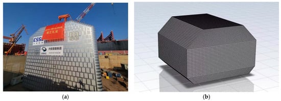
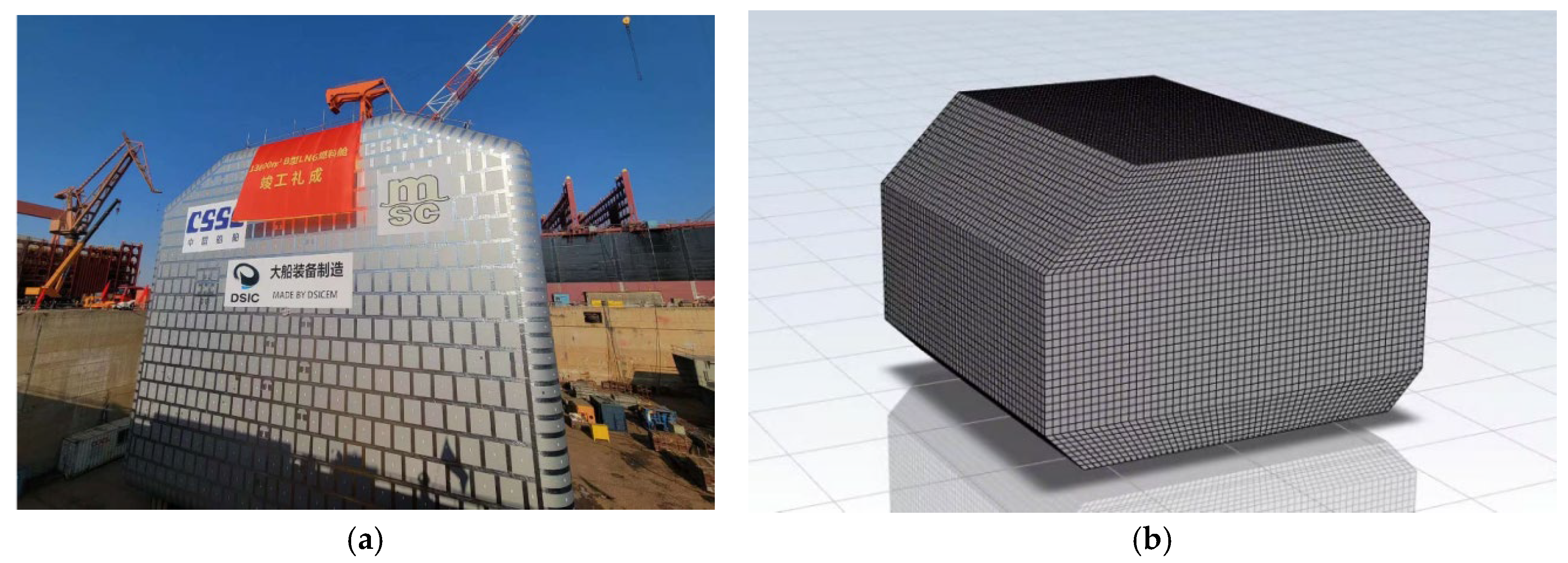
In this study, the liquid cargo hold is modeled based on the new independent LNG B-type cargo hold designed by Hudong Zhonghua Shipbuilding (Group) Co., Ltd., Shanghai, China. The design parameters are detailed, and the corresponding dimension drawing is shown in Figure 1a. The geometric model was created using SOLIDWORKS (2021) software and subsequently imported into ICEM for mesh generation, employing a block meshing approach with refined mesh at critical regions. The coordinate system is established with the origin at the tank center; the x-axis aligns with the ship’s longitudinal direction, the y-axis points upward, and the z-axis is oriented vertically along the ship’s motion. The tank is assumed to be rigid; the effects of deformation and motion of the tank structure under fluid loads are neglected, consistent with prior research. Other studies [31] found that the calculated oscillation pressure, force, and BOG generation were nearly identical across three different mesh densities. To balance accuracy and computational efficiency, we selected a mesh with approximately a model with 46,840 grids for the simulations. As illustrated in Figure 1b, the mesh model of the tank consists entirely of tetrahedral elements, which facilitate accurate computation of fluid dynamics within complex geometries [32].

Figure 1. B-Type LNG fuel tank. (a) actual B-Type LNG fuel tank. (b) Mesh model of the B-Type liquid cargo tank.

3.2. Initial and Boundary Conditions Setup

(1)

Initialization Setup

During initialization, the temperature of the entire fluid domain is set to 111.5 K, the pressure inside the LNG tank is set to 1.01325 × 10 Pa, the ambient air temperature is assumed to be constant at 298 K, the tank walls are treated as rigid bodies, and the gas and liquid inside the tank are static relative to the tank body under the initial conditions. It is assumed that the tank is arranged longitudinally on the ship, meaning the tank’s axis is aligned with the ship’s direction of motion. The four surfaces of the liquid cargo hold-front, rear, left, and right-are defined as force monitoring points, with gas–liquid mixing inside the tank. The motion condition is the ship’s roll condition, which is implemented by writing a User Defined Function (UDF) and using dynamic mesh techniques to apply the motion conditions. A key highlight of our work is the implementation of the UDF feature. Although the material properties remain constant with temperature, the UDF enables real-time heat transfer calculations, allowing the material temperature to be dynamically adjusted based on transient thermal conditions during simulation.

(2)

Boundary Conditions Setup

This study primarily focuses on the internal two-phase flow and phase change thermal performance of LNG within the tank. To simplify the CFD simulation, a model without insulation is employed. In the natural gas industry, the heat ingress into the tank is generally characterized by Equation (10), which is widely used to quantify heat transfer due to environmental conditions and tank design.

$$Q=UA(T_{air}-T_{fliud})$$

(10)

where Q is the heat entering the tank, U is the overall heat transfer coefficient, A is the total surface area of the tank, T_air is the temperature of the ambient air, T_fliud is the temperature of the fluid in the tank.

Therefore, in this study, the third type of boundary condition is applied, where the convective heat transfer coefficient is set as the overall convective heat transfer coefficient (U). Additionally, to simplify the boundary conditions, it is assumed that the overall heat transfer coefficient (U) and the ambient temperature (T_air) are the same for each surface of the simulated tank and do not change over time.

The natural convective heat transfer coefficient for each surface of the insulation system of the liquid cargo hold depends on the empirical equations for natural convection in an infinite space.

For the side surfaces of the liquid cargo hold, the following heat transfer formula is used to calculate the Nusselt number:

$$\begin{gathered} Nu=C{(G{r}_{air}{\mathrm{Pr}}_{air})}^n, C=0.59,n=1/4, (1.43\times {10}^4\le G{r}_{air}\le 3\times {10}^9) \\ C=0.0292,n=0.39, (3\times {10}^9\le G{r}_{air}\le 2\times {10}^{10}) \\ C=0.11,n=1/3, (G{r}_{air}>2\times {10}^{10}) \end{gathered}$$

(11)

For the bottom of the liquid cargo hold (with the cold surface facing downward), the following heat transfer formula is used to calculate the Nusselt number:

$$\begin{gathered} Nu=0.54{(G{r}_{air}{\mathrm{Pr}}_{air})}^{1/4} \\ ({10}^4\le G{r}_{air}{\mathrm{Pr}}_{air}\le {10}^7) \end{gathered}$$

(12)

$$\begin{gathered} Nu=0.15{(G{r}_{air}{\mathrm{Pr}}_{air})}^{1/4} \\ ({10}^7\le G{r}_{air}{\mathrm{Pr}}_{air}\le {10}^{10}) \end{gathered}$$

(13)

For the top surface of the liquid cargo hold (with the cold surface facing upward), the following heat transfer formula is used to calculate the Nusselt number:

$$\begin{gathered} Nu=0.27{(G{r}_{air}{\mathrm{Pr}}_{air})}^{1/4} \\ ({10}^5\le G{r}_{air}{\mathrm{Pr}}_{air}\le {10}^{10}) \\ G{r}_{air}={\displaystyle \frac{g{\alpha }_V\mathsf{\Delta }T{l}^3}{{\nu }_{air}^2}} \\ Nu={\displaystyle \frac{h_{i,c}l}{{\lambda }_{air}}} \end{gathered}$$

(14)

In the above equation, λ_air is the thermal conductivity of air, g is the gravitational acceleration, v_air is the dynamic viscosity of air, α_v is the volumetric expansion coefficient of air, T is the temperature difference between the insulation layer and the external environment, Pr_air is the Prandtl number of air, l is the characteristic length of the surface, Gr_air is the Grashof number for air.

Based on the above equation, the natural convection heat transfer coefficient at the corresponding location of the simulated storage tank can be calculated h. Subsequently, the overall heat transfer coefficient method from the literature is used to calculate the total heat exchange of the insulation system. Therefore, based on the equation, Q = UA (T_air − T_fliud), when the insulation layer is 400 mm thick and has a thermal conductivity of 0.025 W/(m·K), the overall heat transfer coefficient (U) can be determined as 0.128 W/(m²·K).

3.3. Sloshing Model

The ship’s sway is complex, primarily caused by ocean waves, such as transverse waves, wind-induced waves, and current forces. The process involves hydrodynamic lateral water forces displacing the vessel from equilibrium, leading to periodic side-to-side oscillations (sway). Additional factors, including wind forces, speed variations, and initial disturbances from operational actions, can further trigger or amplify the sway motion. These combined effects result in the vessel’s cyclic horizontal oscillations.

The emergency stop test is a vital procedure to ensure the safety of ship navigation, as it evaluates the vessel’s capability to stop rapidly and safely in emergency scenarios. In this study, the test is divided into three distinct motion conditions: straight-line deceleration, ship braking during turning, and ship pitching. The primary focus is on examining the thermodynamic phenomena associated with fluid sloshing in the B-type liquid cargo hold under each condition. Specifically, the study aims to elucidate how different ship motions influence fluid behavior, including thermal and pressure variations, which are critical for ensuring operational safety. Furthermore, the findings can provide valuable insights for the optimization of tank design to mitigate risks related to fluid sloshing during emergency maneuvers.

(1)

Straight-line Deceleration Braking Condition

Under the straight-line deceleration braking condition, it is assumed that the ship maintains a fixed heading and decelerates exclusively along a straight trajectory. This deceleration induces fluid sloshing within the cargo hold, resulting from the combined effects of inertia and the chamber’s structural constraints. To simulate this process accurately, the ship’s motion profile is designed as specified in Table 1, where the hull undergoes a constant deceleration of −19.6 m/s² and comes to a complete stop within one second. The fluid sloshing excitation is modelled using the User-Defined Function (UDF) feature in FLUENT, which provides precise control over the dynamic forcing that corresponds to the ship’s deceleration. This methodology facilitates a comprehensive analysis of the fluid’s response, including pressure distribution and flow behavior, which are essential for safety evaluations and the optimization of tank design.

Table 1. Motion State at Different Time Points.

Time t (s)	Motion State
Before 0 s	Moving at a constant speed of 19.6 m/s
From 0 s to 1 s	Decelerating with an acceleration of −19.6 m/s2
After 1 s	The liquid cargo hold comes to rest

(2)

Ship Braking and Turning Condition

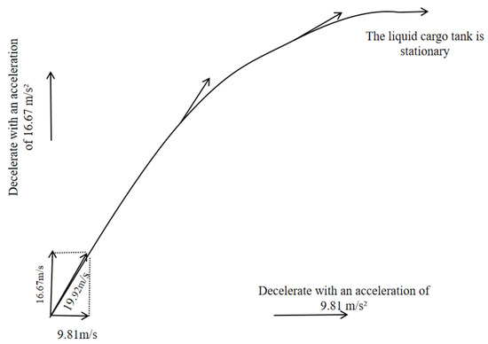
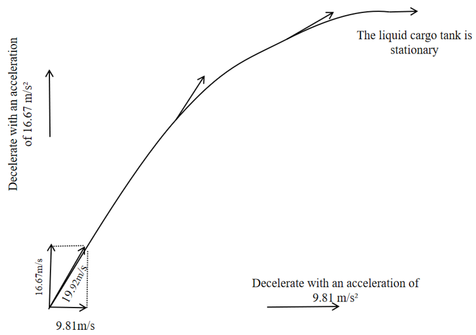
In the ship braking and turning condition, it is assumed that during the deceleration process, the helmsman fully deflects the rudder (either left or right). The rudder force is utilized to deflect the ship, increase hydrodynamic resistance, and assist in slowing down the vessel. The motion state of the ship during the simulation is illustrated in Figure 2. Specifically, it is assumed that the liquid cargo hold experiences deceleration in the x-direction with an acceleration of 9.81 m/s² and in the y-direction with a velocity reduction of 16.67 m/s. After one second, the cargo hold comes to a complete halt. The oscillation excitation caused by this maneuver is modeled using the User-Defined Function (UDF) feature in FLUENT, enabling precise control of the dynamic forcing corresponding to the combined deceleration and turning actions. This approach allows for detailed investigation of fluid sloshing behaviors and pressure variations, which are crucial for safety assessments and tank structure design optimization.

Figure 2. Ship Braking and Turning Condition Trajectory.

(3)

Ship Pitching Condition

In the emergency stop test, after the ship’s deceleration concludes, it experiences a pitching motion driven by its own inertia and external wind-wave currents. This motion causes the liquid inside the cargo hold to oscillate primarily along the longitudinal (forward–backward) direction, which can impose significant impact loads on the transverse bulkheads. Consequently, it is crucial to investigate the fluid oscillation mechanisms within the rectangular liquid hold subjected to longitudinal excitation. The external excitation in the pitching condition is modelled as simple harmonic motion, described by Equation (15). The pitching excitation is implemented using the User-Defined Function (UDF) feature in FLUENT, allowing precise control of the acceleration profile corresponding to the pitching motion. This setup facilitates a detailed analysis of the fluid’s dynamic response to longitudinal excitation, providing insights into pressure fluctuations and flow patterns that are vital for structural safety and design optimization.

$$Y=A\sin (2\pi fT)$$

(15)

where A is the amplitude of external excitation, f is the frequency of external excitation, and Y is the displacement of external excitation.

3.4. Simulation Method Settings

The VOF method is utilized to simulate fluid sloshing within the cargo tank, with solver parameters specified in Table 2. The residual convergence criteria are set to 1 × 10⁻⁴ for the continuity, momentum, volume fraction, and turbulence equations to ensure numerical stability and accuracy. For the energy equation, a more stringent residual criterion of 1 × 10⁻⁸ is adopted to precisely capture thermal effects. The iterative numerical solution is considered converged when the residuals-measuring the difference between successive iterations-drop below this threshold. This high-precision criterion ensures that the key flow variables have stabilized to a very small tolerance, providing reliable and accurate simulation results. The transient simulations employ a time step of 5 × 10⁻³ s, effectively resolving dynamic fluid motions. The environmental pressure is maintained at atmospheric pressure of 1.013 × 10⁵ Pa, representing standard atmospheric conditions. Collectively, these settings enable a stable and accurate analysis of fluid–structure interactions and phase change phenomena inside the cargo hold.

Table 2. Solver Settings.

Parameters	Options
Computational Mode	3D Double Precision
Solver Type	Pressure-Based Solver
Time Type	Transient Problem
Physical Model	Multiphase Flow VOF Model
Turbulence Model	Standard k-epsilon Model
Materials	Gas as the Primary Phase, Liquid as the Secondary Phase
Computational Method	Pressure–Velocity Coupling SIMPLE Algorithm
Pressure Discretization Scheme	Brute Force Weighted Algorithm
Time Discretization Scheme	First-order Implicit Scheme
Time Step	0.005 s

3.5. Model Verification

Compares the analytical solution for the first-order natural frequency of the LNG cargo tank model with the numerical simulation results to validate the accuracy of the computational approach. The analytical expression used to calculate the natural frequency of the LNG cargo tank is defined as follows:

$$f={\displaystyle \frac{\sqrt{\frac{g\pi }{b}\tanh (\frac{\pi h}{b})}}{2\pi }}$$

(16)

In Equation (16), g represents the gravitational acceleration, b is the effective sloshing length, and h is the liquid fill height.

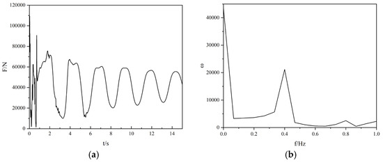
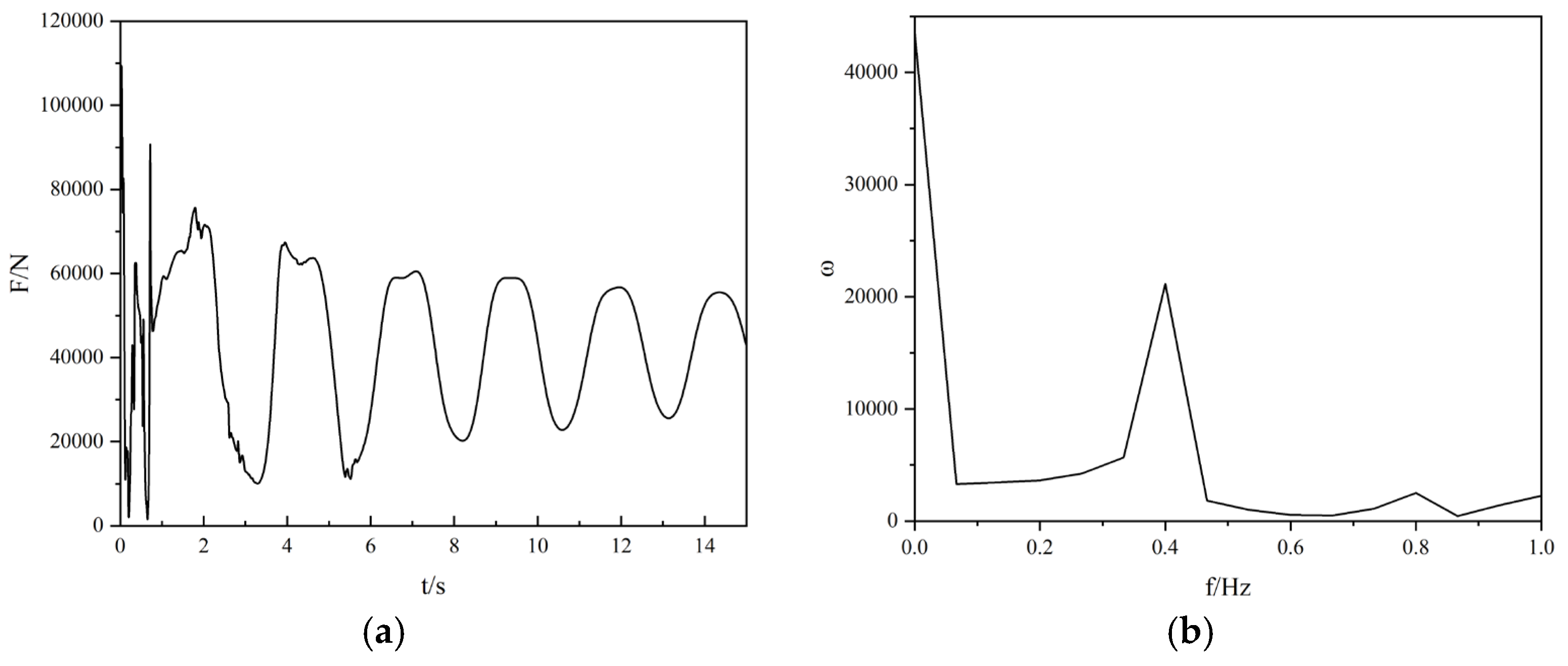
Using Equation (16), the first-order natural frequency of the LNG cargo tank at a 50% fill level is calculated to be 0.404 Hz. Under the emergency stop braking condition at a 50% fill level, the fluid inside the tank oscillates at its natural frequency starting from t = 0 when the tank comes to rest. The variation in the force exerted by the fluid on the forward bulkhead is shown in Figure 3a. The force exhibits periodic changes, with the amplitude gradually decreasing over time. The oscillation frequency of the fluid inside the LNG cargo tank, obtained from spectral analysis, is shown in Figure 3b. The first-order oscillation frequency of the fluid is approximately 0.4 Hz. The numerical simulation results for the first-order natural frequency of the simulation model closely match the analytical solution [33], thereby verifying the accuracy of the model.

Figure 3. Numerical analytical solution result. (a) Variation of the fluid force on the forward bulkhead over time. (b) Amplitude–frequency characteristic curve after FFT transformation.

4. Results and Discussion

4.1. Static Evaporation in the Liquid Cargo Tank

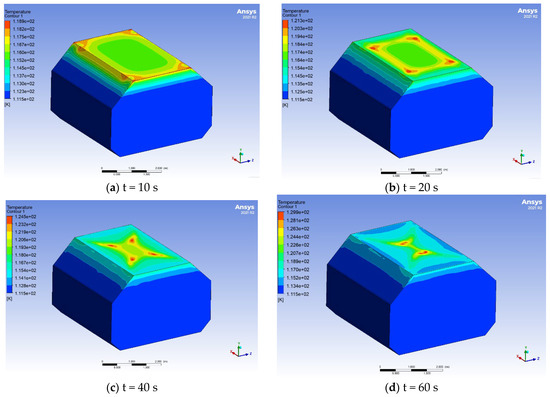
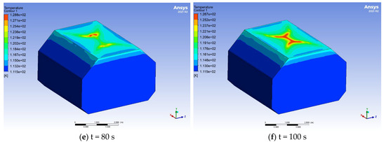
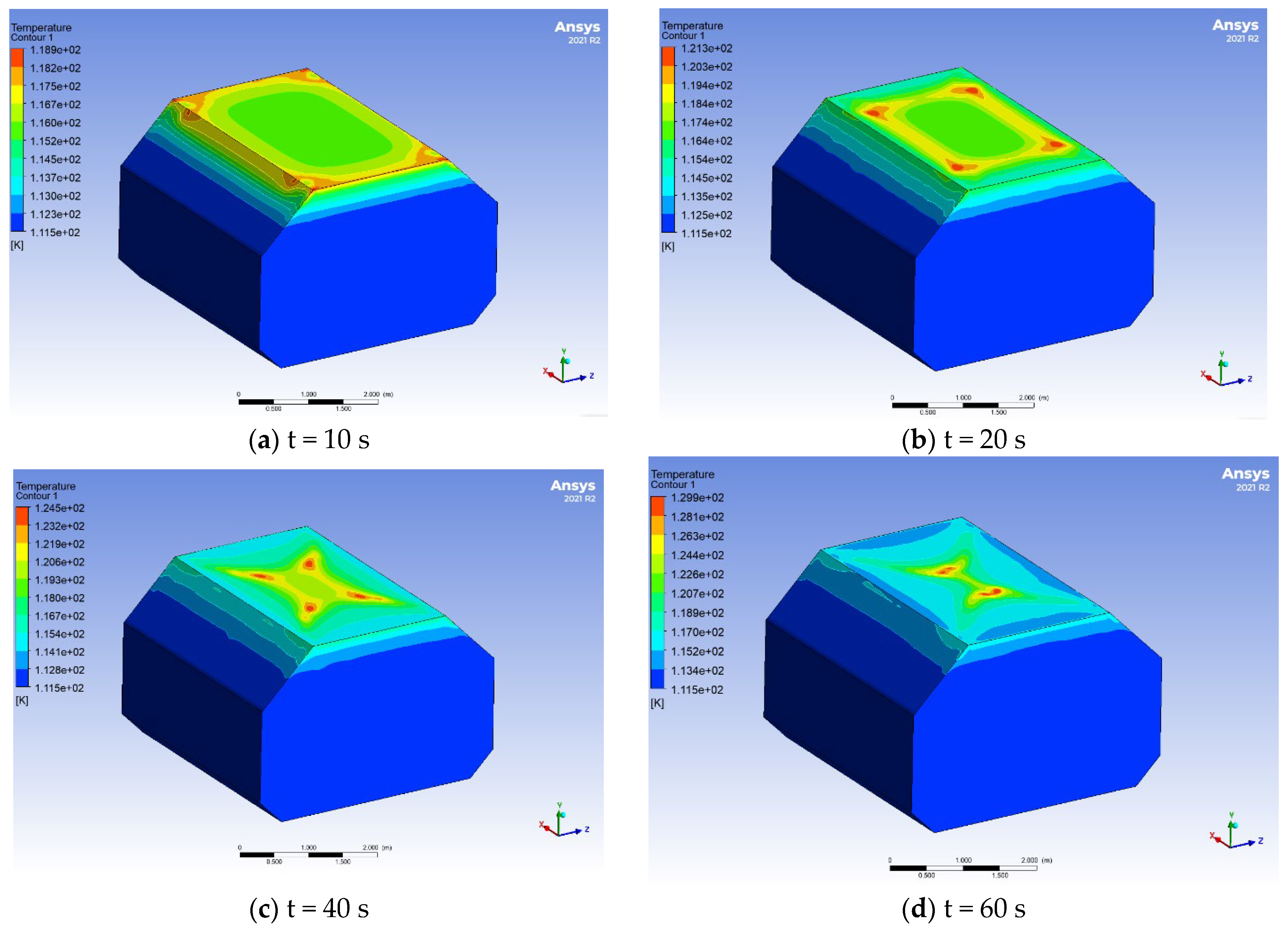
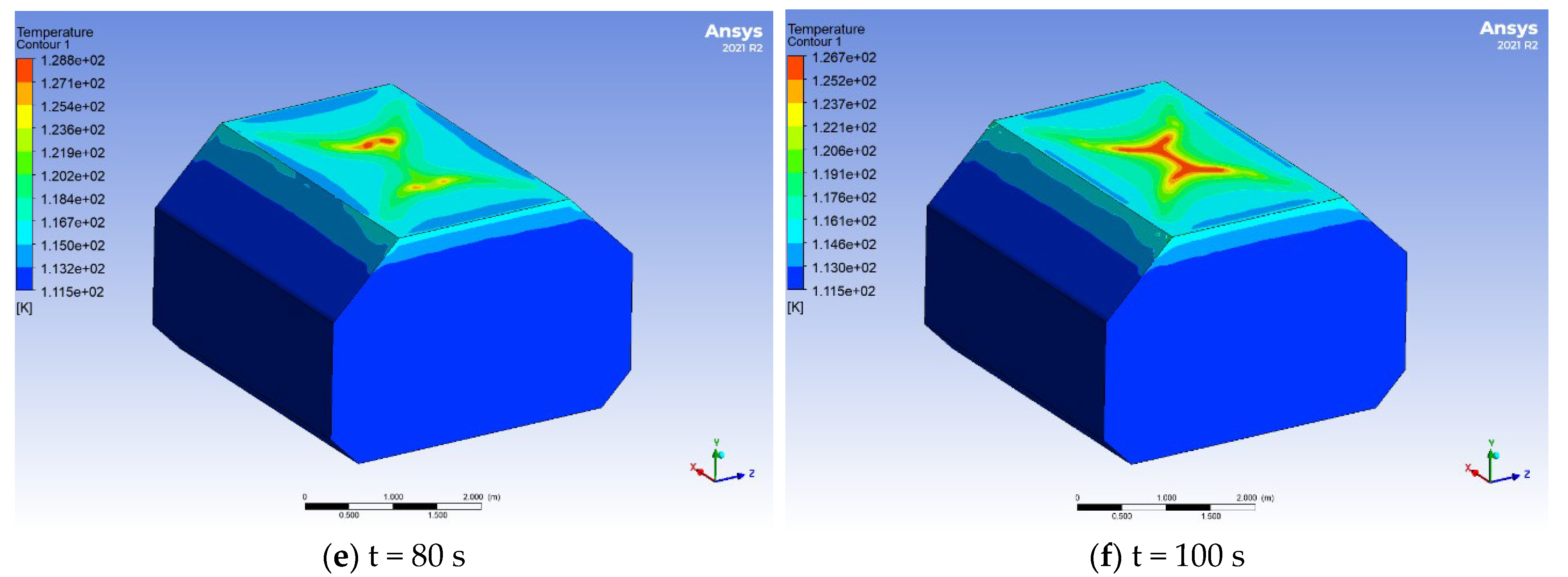
Figure 4 presents the temperature distribution on the tank wall over a duration of 100 s. Prior to t = 10 s during the static evaporation process, high-temperature gas is predominantly located at the four sharp corners at the top of the tank. This distribution is attributed to the structural features of the Type B tank, where these sharp corners facilitate heat exchange among three surfaces and the surrounding air, leading to an initial accumulation of high-temperature gas at these points. After t = 10 s, during the same static evaporation process, the high-temperature gas begins to migrate toward the center of the tank’s top region. This movement occurs because the high-temperature gas exhibits comparatively lower pressure, and is compressed by the surrounding gas, which gradually pushes it inward. Consequently, the temperature distribution at the top temporarily forms an “X” shape as the high-temperature regions converge toward the center. This temperature evolution indicates the dynamic heat transfer mechanisms governing the evaporation process within the tank, offers valuable insights into the critical temperature distribution patterns that influence LNG containment system safety and thermal management strategies.

Figure 4. Temperature distribution of the gas–liquid mixture during static evaporation in the liquid cargo tank at an 80% filling ratio.

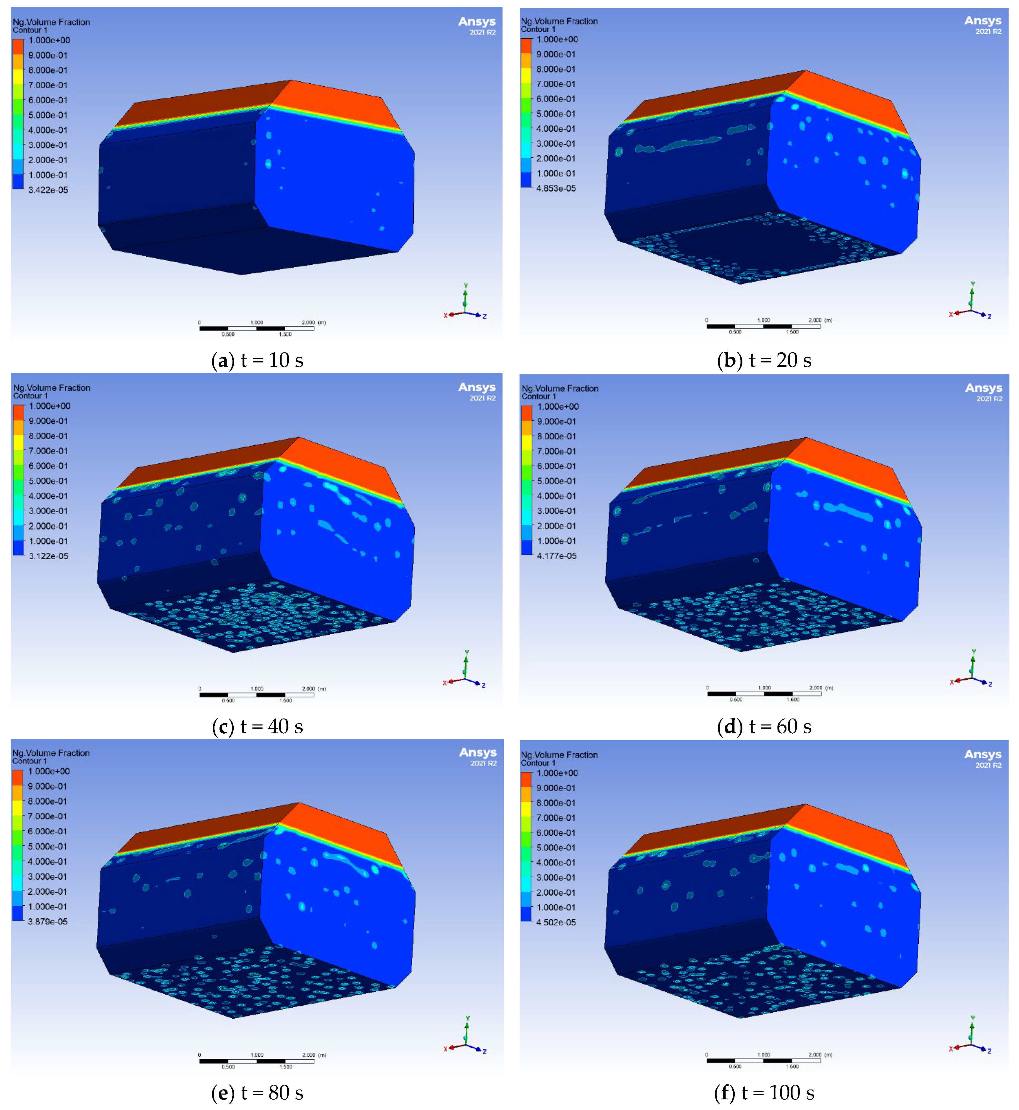
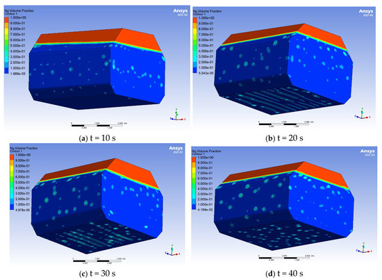
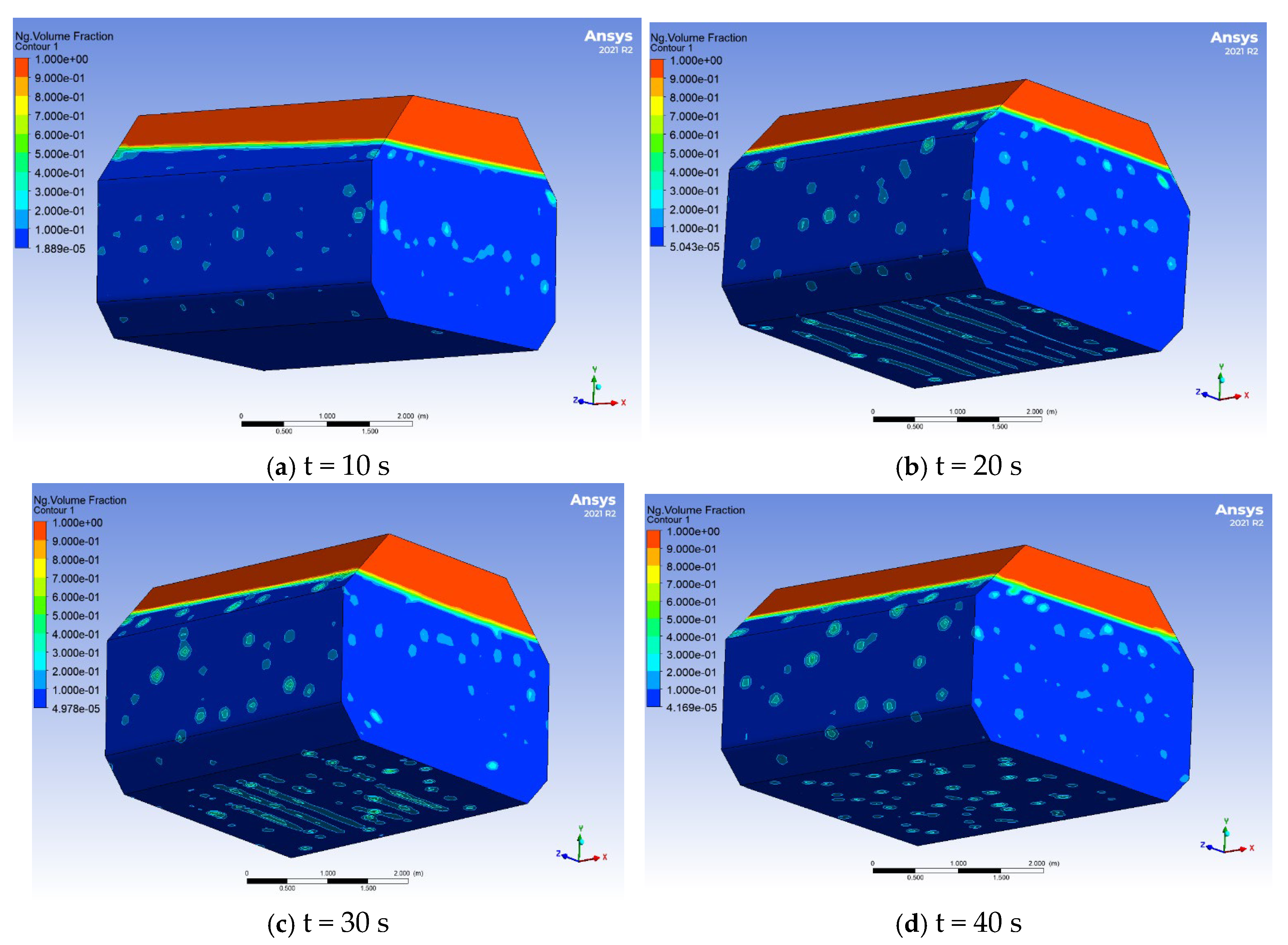
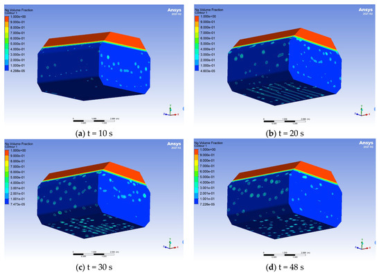
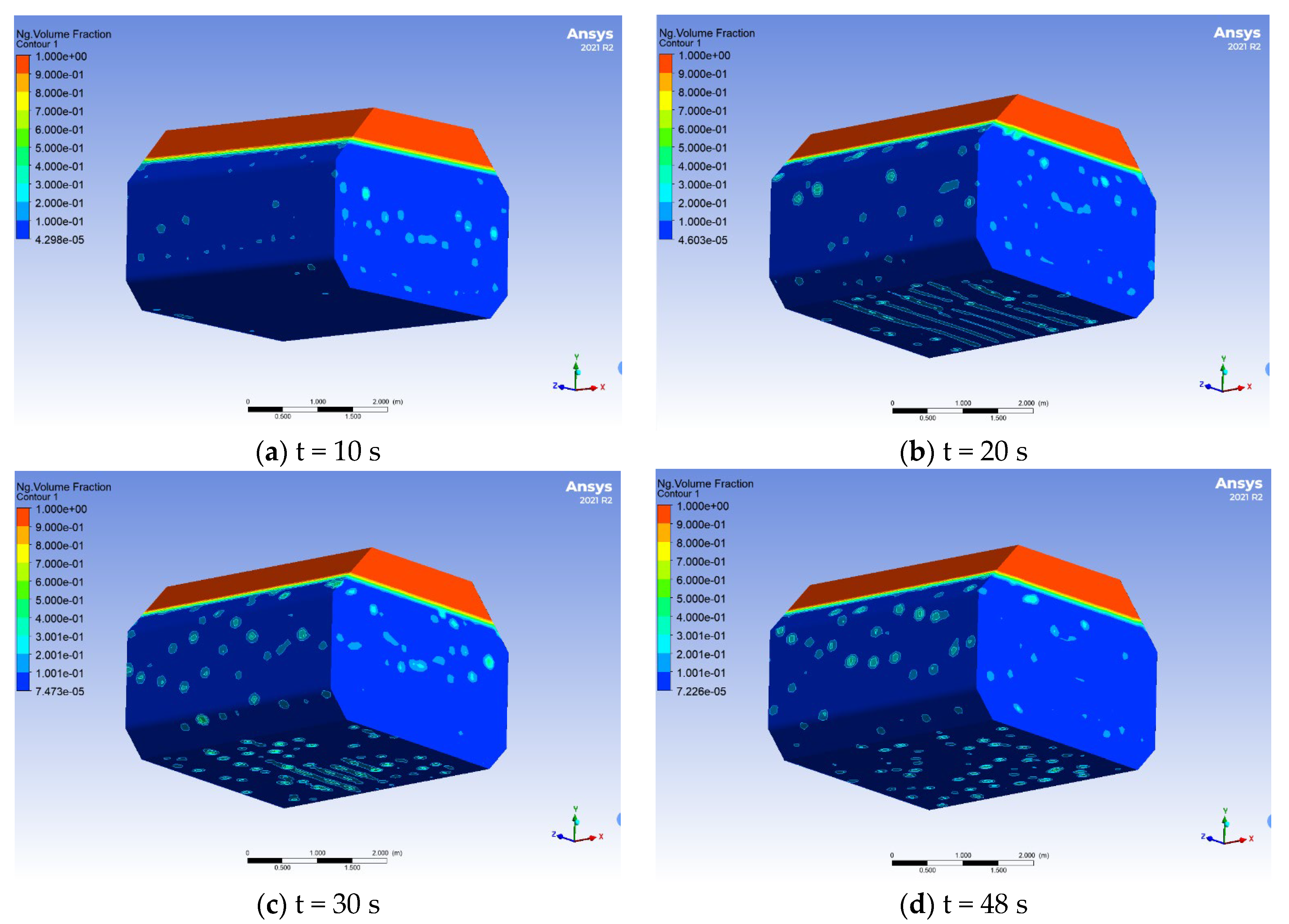
During the initial phase of static evaporation (at t = 10 s), a small number of bubbles are observed on the front and rear endcaps, as well as along the sidewalls of the liquid cargo tank. These bubbles are primarily concentrated near the tank edges, with no bubbles detected at the bottom. Progressively (t = 20 s), the bubble population increases significantly, appearing at the bottom and distributed along the outer perimeter; however, no bubbles are observed at the center of the bottom surface. Additionally, larger elongated bubbles are visible on the sidewalls, indicating that the evaporation has transitioned into the nucleate boiling phase [34]. At extended time scales (t = 40 s), the bottom of the tank is extensively covered with bubbles, and the amount of evaporated gas on the endcaps and sidewalls has further increased. This evolution of bubble formation and distribution reflects the progression of phase change mechanisms within the tank, providing insights into the evaporation dynamics and thermal behavior in LNG storage systems.

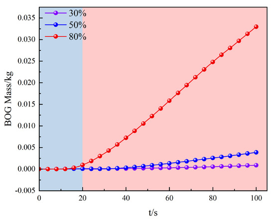
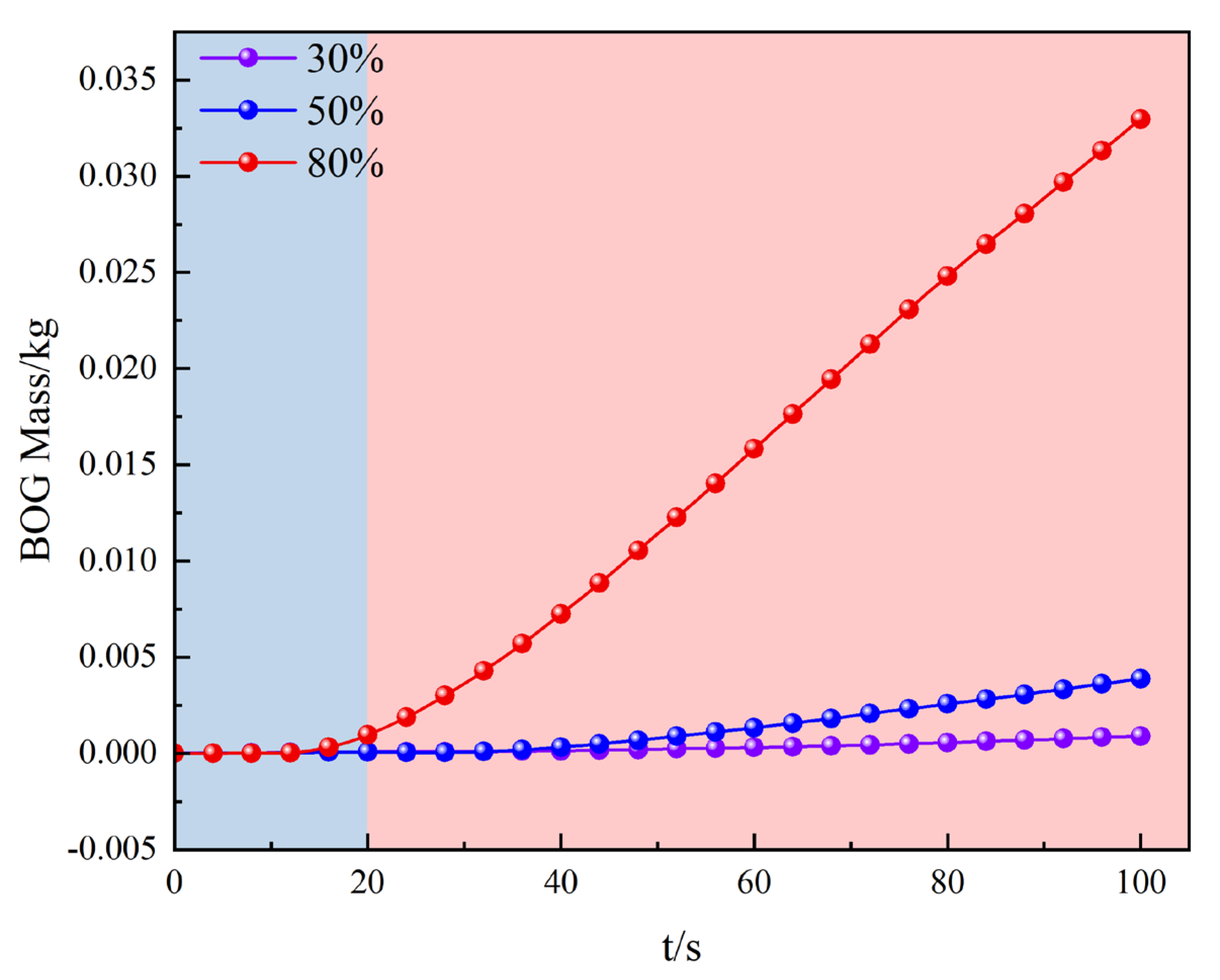
In the static evaporation experiments, three fill levels-30%, 50%, and 80%-were analyzed to assess Boil-Off Gas (BOG) generation within a Type B LNG cargo tank. Figure 5 and Figure 6 depict BOG production over time at each level. At 30% fill, BOG forms immediately at evaporation onset, lacking the relaxation period seen at higher levels. This occurs because the smaller LNG volume at the tank bottom absorbs heat more effectively from the ambient air due to the tank’s structure, resulting in rapid BOG generation that readily mixes with the gas phase, thereby reducing condensation losses. Specifically, approximately 0.0009 kg of BOG is produced within 100 s at 30%, indicating limited heat transfer owing to the reduced liquid volume. Conversely, at 50% fill, the BOG pattern resembles that at 30%, although featuring an initial relaxation phase where evaporation and condensation balance before net BOG increases. Over 100 s, about 0.0038 kg of BOG is generated, an intermediate amount compared to the other levels. At 80% fill, A large amount of BOG forms. This trend suggests that higher fill levels lead to greater heat absorption by the LNG, resulting in increased BOG production during static conditions. Overall, these results confirm that larger fill levels enhance heat intake and BOG generation, emphasizing the impact of volume on phase change dynamics in LNG storage.

Figure 5. Distribution of gas–liquid phases in the liquid cargo tank at 80% fill level during static evaporation at different time steps.

Figure 6. BOG generation in the liquid cargo tank at 30% fill level during static evaporation at different time steps.

4.2. Impact Load of Fluid Sloshing on the Liquid Cargo Tank

4.2.1. Linear Deceleration Braking Condition

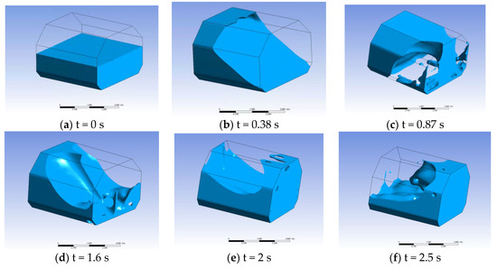
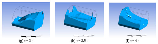
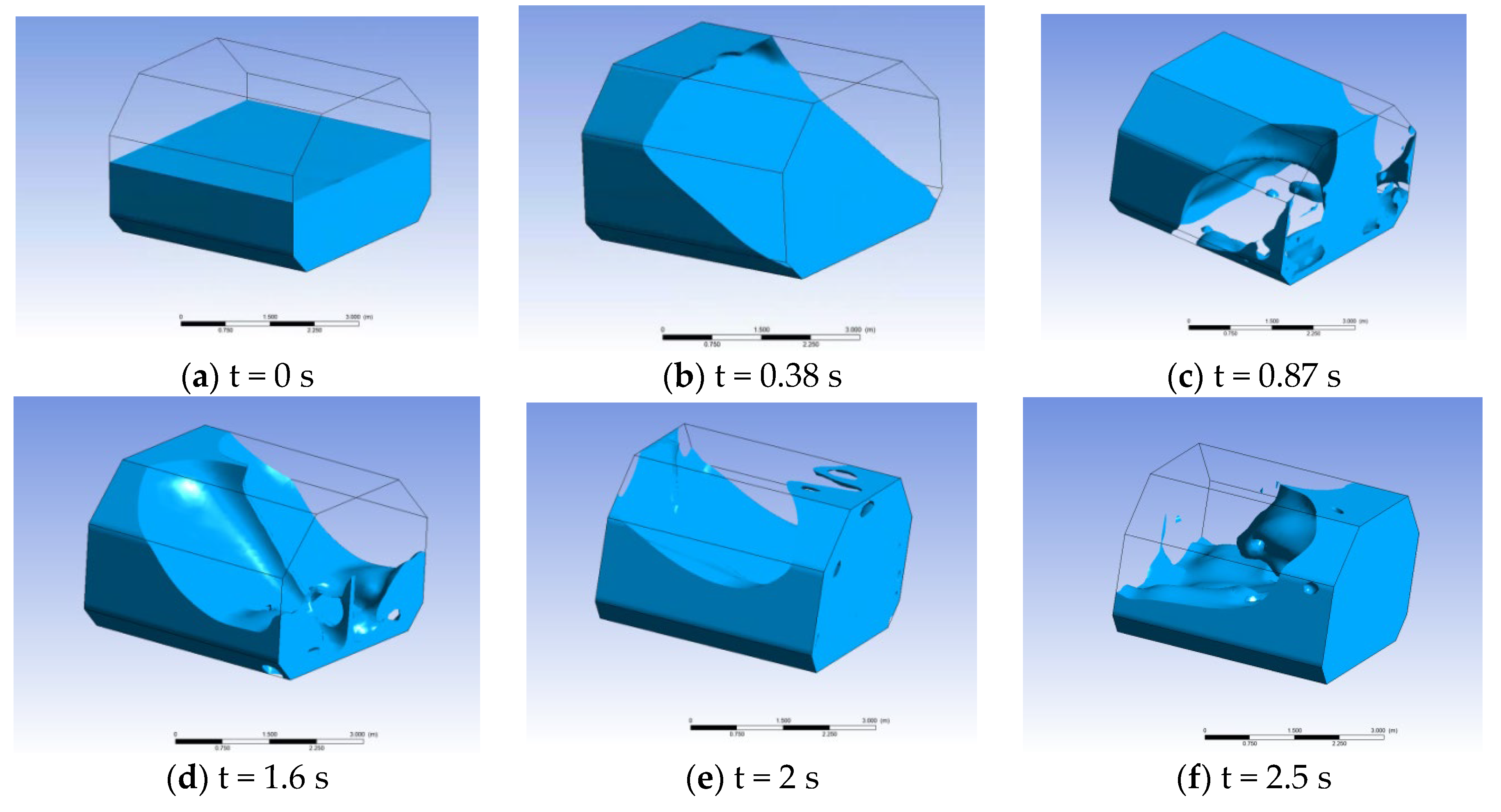
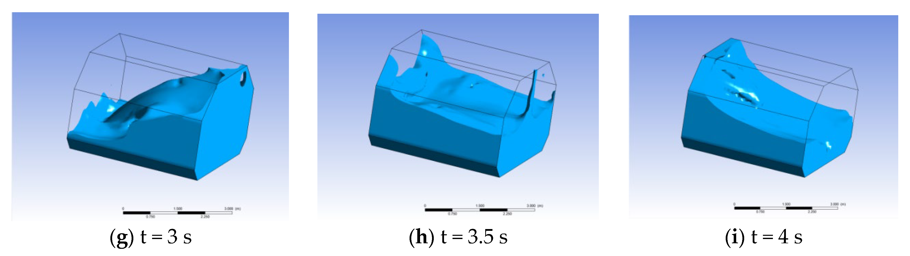
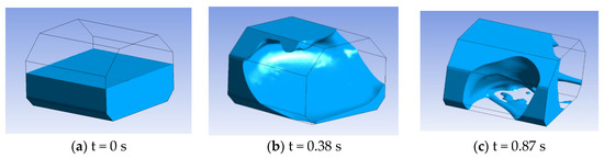
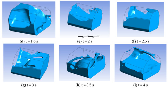
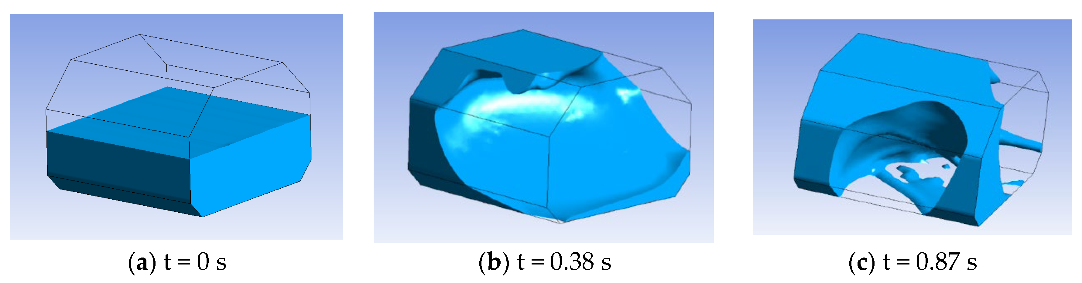
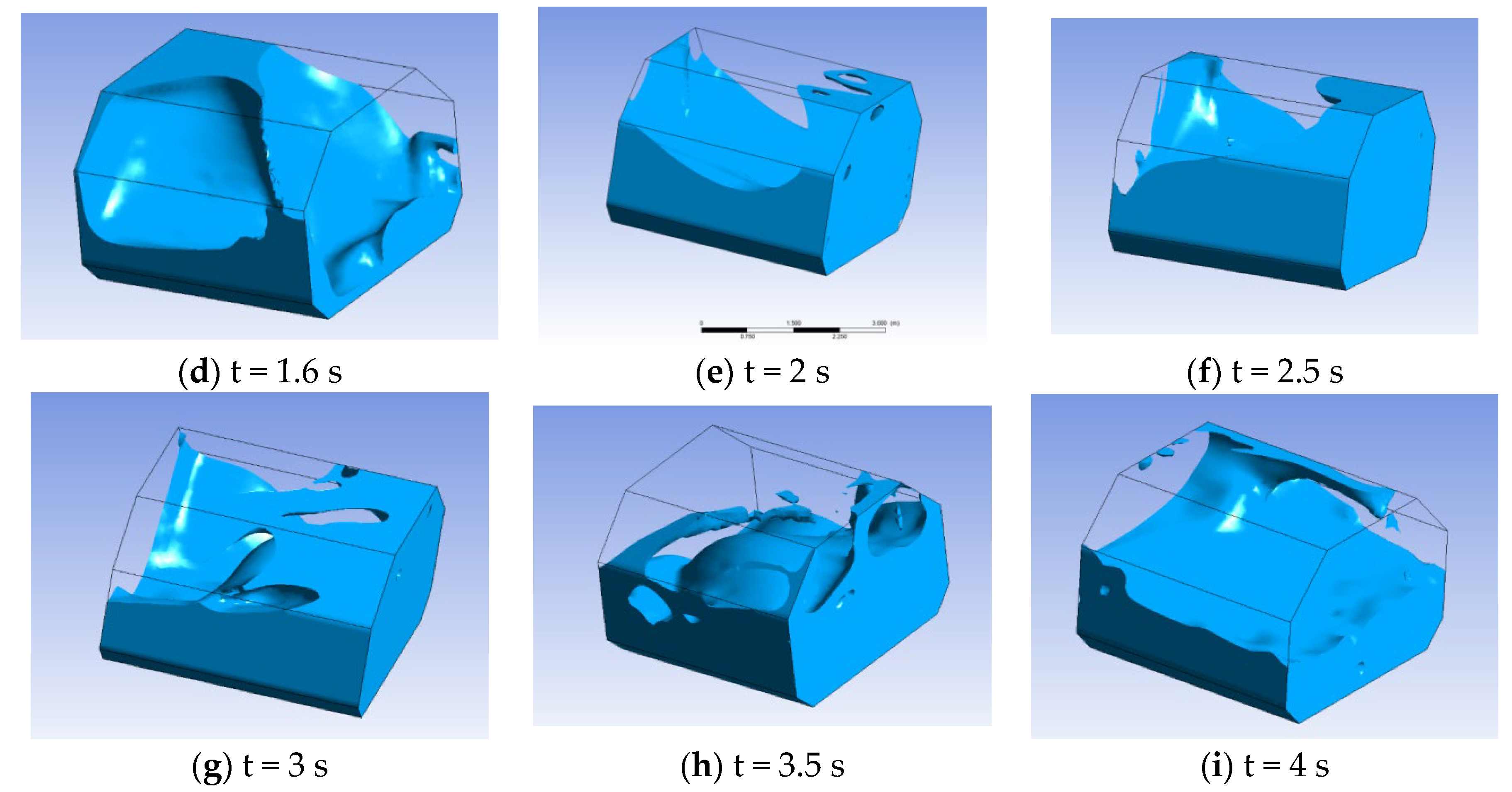
The fluid motion within the cargo tank under emergency braking conditions is depicted in Figure 7. During deceleration, the fluid within the cargo tank exhibits significant inertial effects, moving counter to the direction of acceleration and thereby inducing sloshing phenomena. This fluid motion results in impact forces exerted on the tank walls, which can be quantified by integrating the pressure distribution over the respective surface areas. As illustrated, at t = 0 s (Figure 7a), the tank is in a state of uniform motion prior to braking. By t = 0.38 s (Figure 7b), the inertial effect causes the fluid to impact the front bulkhead.

Figure 7. Cloud plots of fluid sloshing at different time instances in the liquid cargo tank.

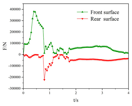
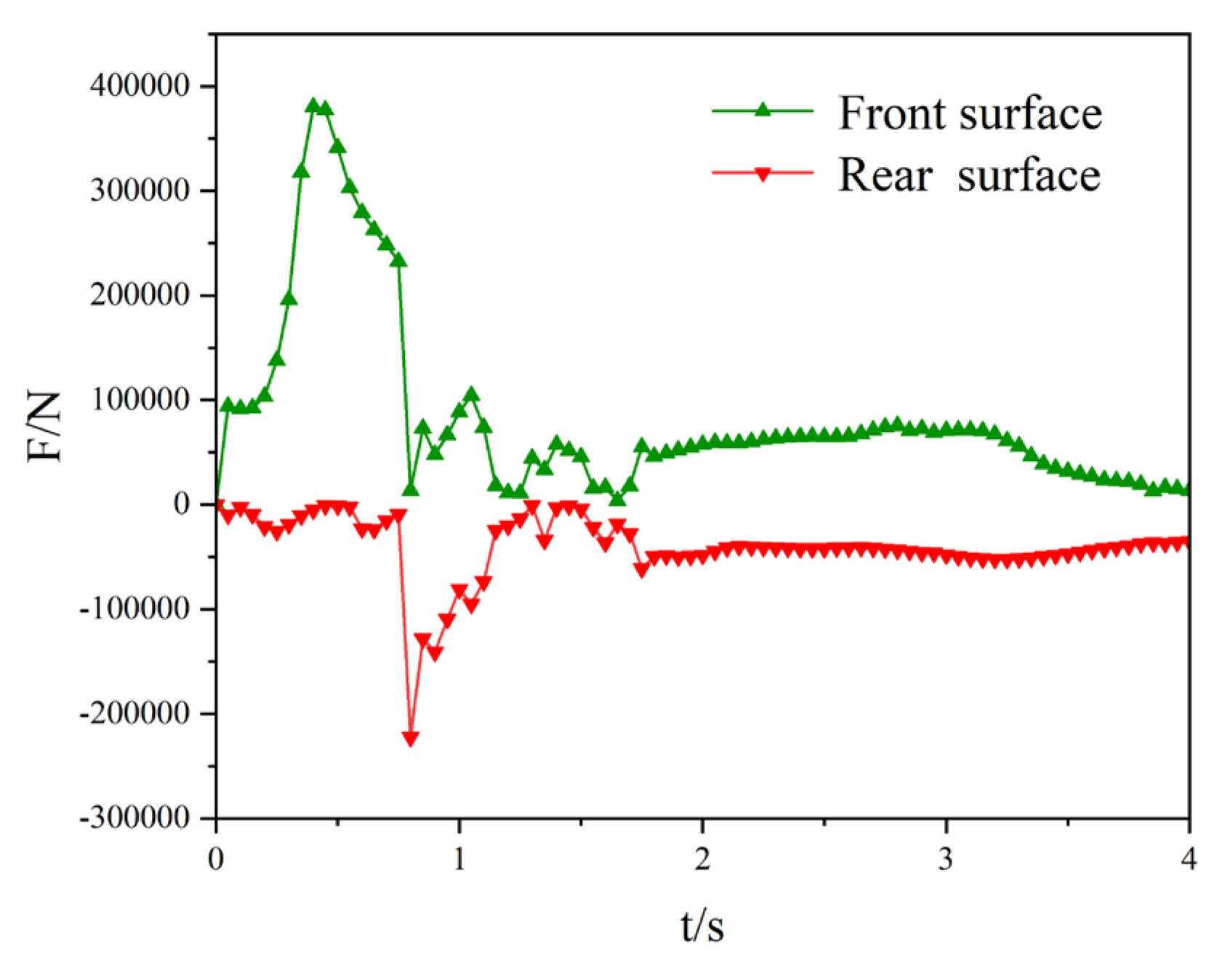
As depicted in Figure 8, where the impact force peaks at F_max = 394,909.41 N. The fluid tends to move forward, but is impeded by the front bulkhead, being forced upward along its surface. Consequently, at this time, the total volumetric force from the entire fluid domain is transmitted to the front bulkhead, resulting in the maximum impact force. When deceleration ceases at t = 0.87 s, the fluid flows backward toward the rear bulkhead, which experiences a maximum impact force of 222,628.51 N-considerably less than that on the front bulkhead due to the impact location and fluid dynamics. Figure 7d–i demonstrate that, during deceleration, the fluid oscillates back and forth within the tank, gradually settling to rest, with the impact forces diminishing to zero over time. This dynamic process highlights the significant influence of inertial effects on fluid–structure interaction during emergency braking.

Figure 8. Variation of the impact force exerted on the liquid cargo tank with time.

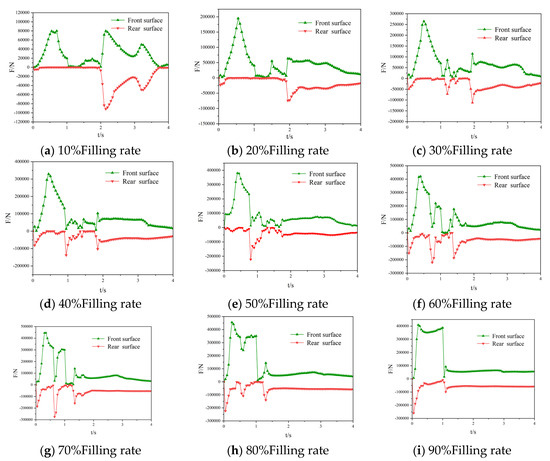
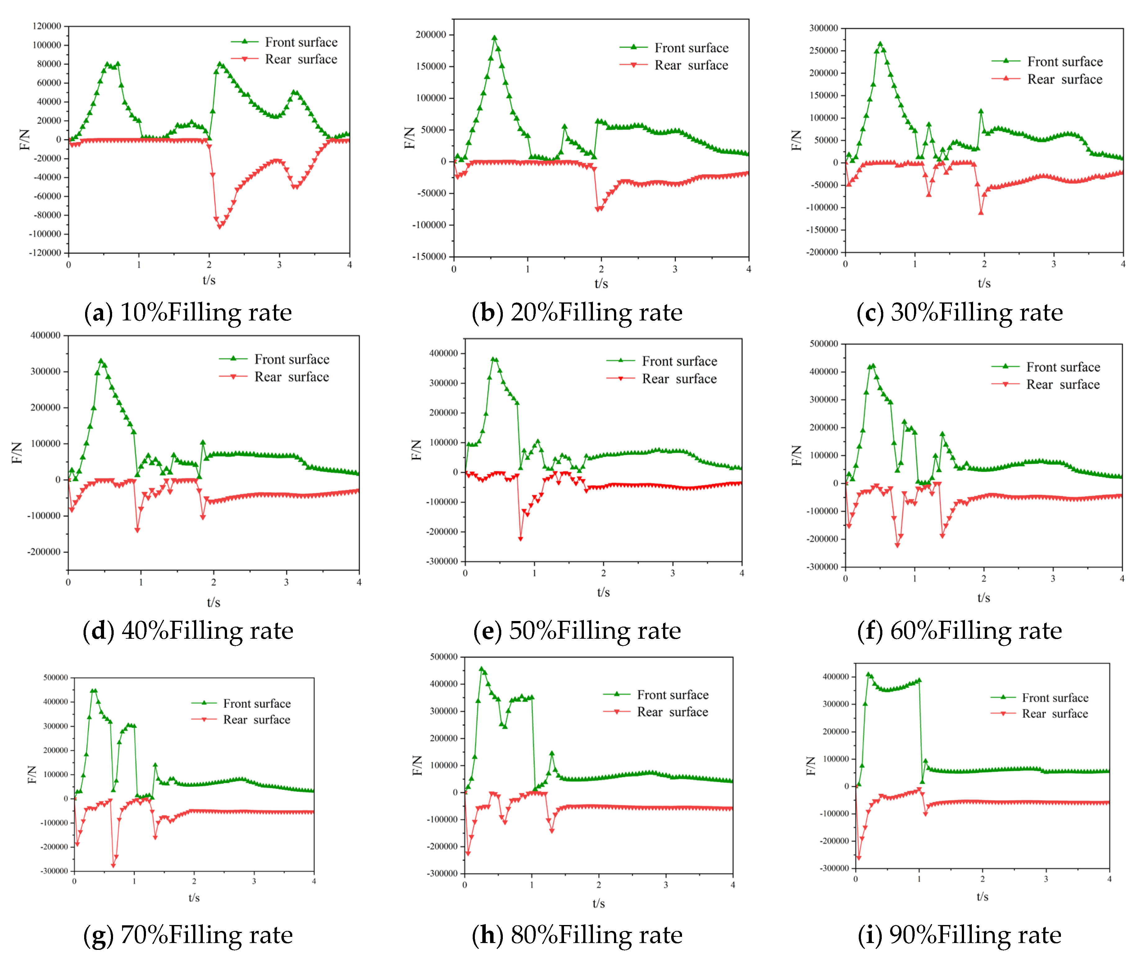
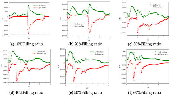
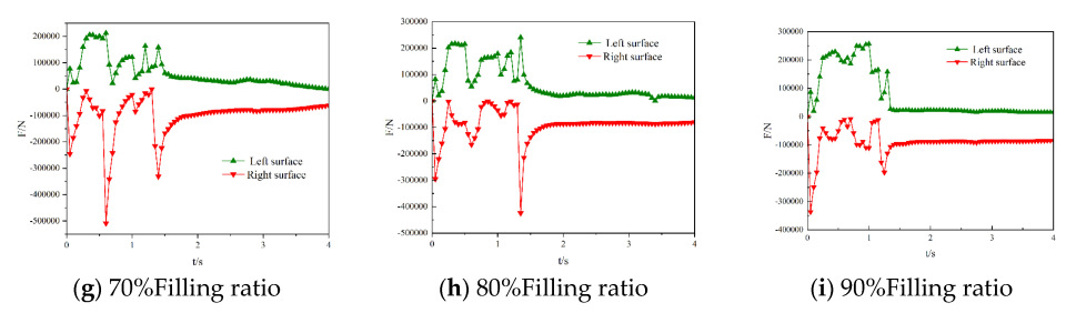
The filling rate of the liquid cargo tank, defined as the ratio of the liquid height to the total tank height, is a critical parameter in studying sloshing phenomena. A control variable approach is employed, wherein the filling rate is systematically varied while other parameters remain constant, to investigate its effect on the maximum impact force exerted on the tank. Nine filling conditions are selected: 10%, 20%, 30%, 40%, 50%, 60%, 70%, 80%, and 90%. Figure 9a–i illustrate the time-dependent impact forces on both the front and rear heads across these nine filling rates. This analysis provides insight into how different liquid levels influence the magnitude and timing of slosh-induced impacts, which are vital for ensuring structural safety and optimal tank design.

Figure 9. Impact force curves on the liquid cargo tank at different filling rates.

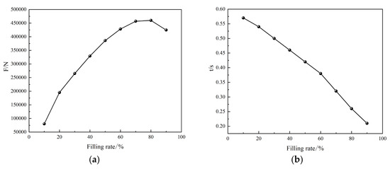
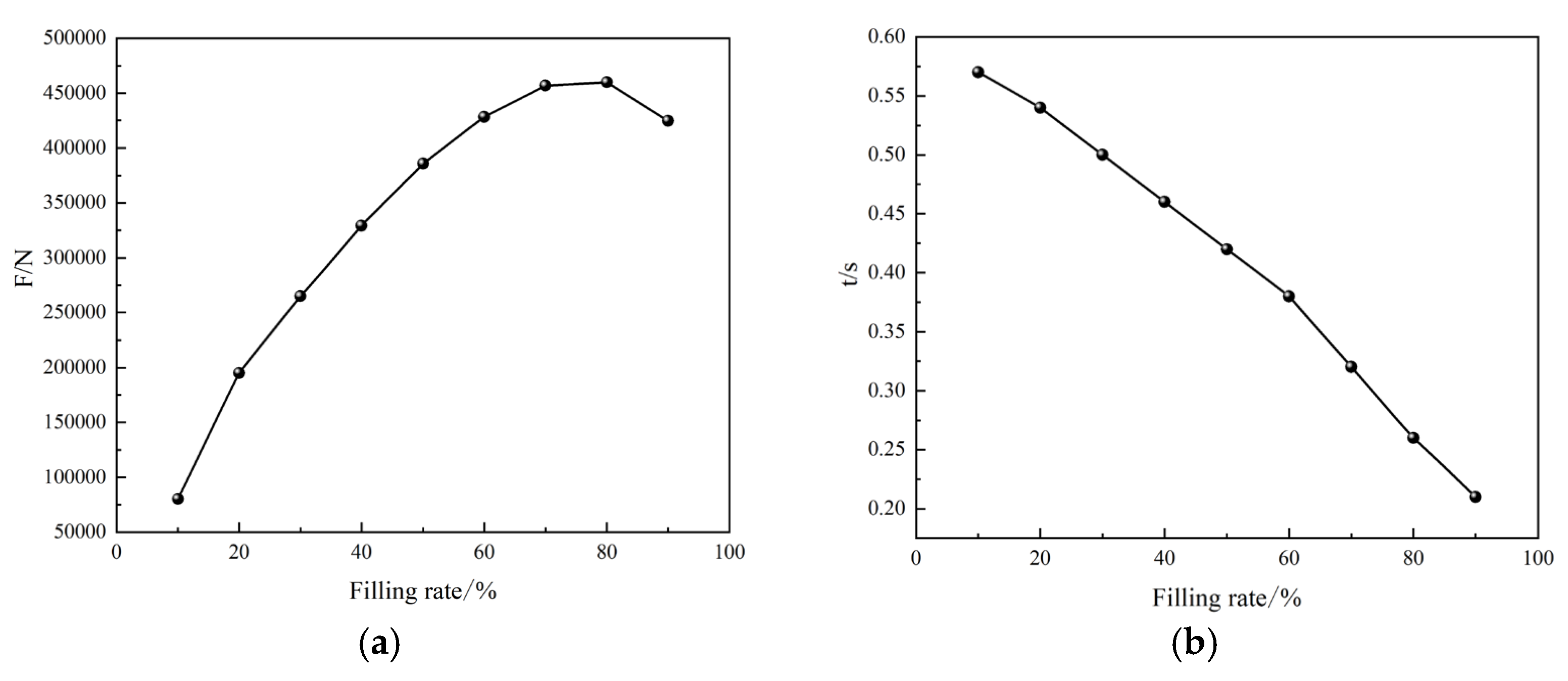
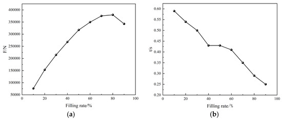
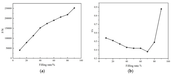
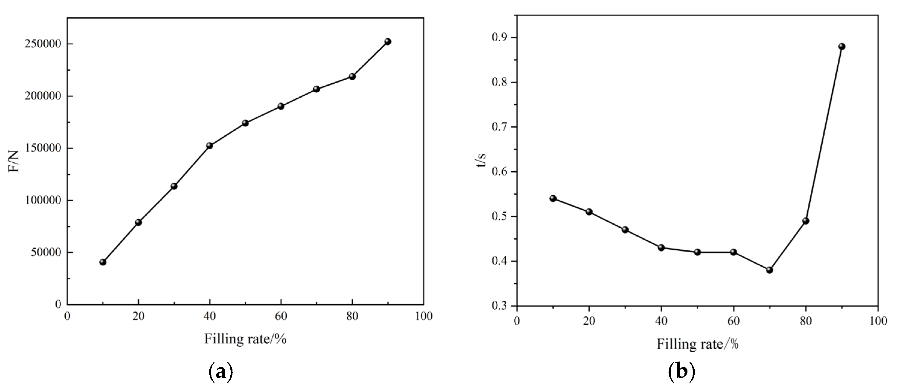
As depicted in Figure 9, at filling rates of 60%, 70%, and 80%, a double peak phenomenon is observed in the maximum impact force, which indicates intensified sloshing behavior. In practical LNG vessel operations, it is advisable to avoid operating within these filling range to mitigate potential structural risks associated with high-impact forces. Figure 10 shows that, during vessel emergency braking, the impact force on the liquid cargo tank generally increases with the filling rate, reaching its peak at approximately 80%. Afterwards, the impact force gradually decreases but does not drop to zero. This phenomenon results from the strong correlation between the volumetric forces exerted by the liquid and the inertial forces generated at the free surface. This trend suggests that for filling rates up to 80%, the impact force correlates positively with the liquid volume, as more liquid volume results in greater inertial effects and sloshing intensity. Beyond 80%, the liquid occupies a larger proportion of the tank, limiting free liquid movement and thereby stabilizing the sloshing motion and associated impact forces. These findings underscore the importance of carefully selecting filling levels to balance operational efficiency and structural safety considerations in LNG transport.

Figure 10. Impact force under different filling rates. (a) Maximum impact force on the liquid cargo tank under different filling rates. (b) Time of occurrence of the maximum impact force under different filling rates.

As illustrated in Figure 10, the time at which the maximum impact force occurs decreases with increasing filling rate, from 0.57 s at lower fill levels to 0.21 s at higher levels. This trend indicates that as the liquid volume becomes larger within the cargo tank, the area of significant liquid movement diminishes, causing the fluid to exert its entire volumetric force on the front bulkhead earlier in the deceleration process. Based on this pattern, it can be inferred that at a full fill (100%), the maximum impact force would occur immediately.

4.2.2. Braking and Turning Deceleration Condition

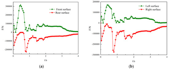
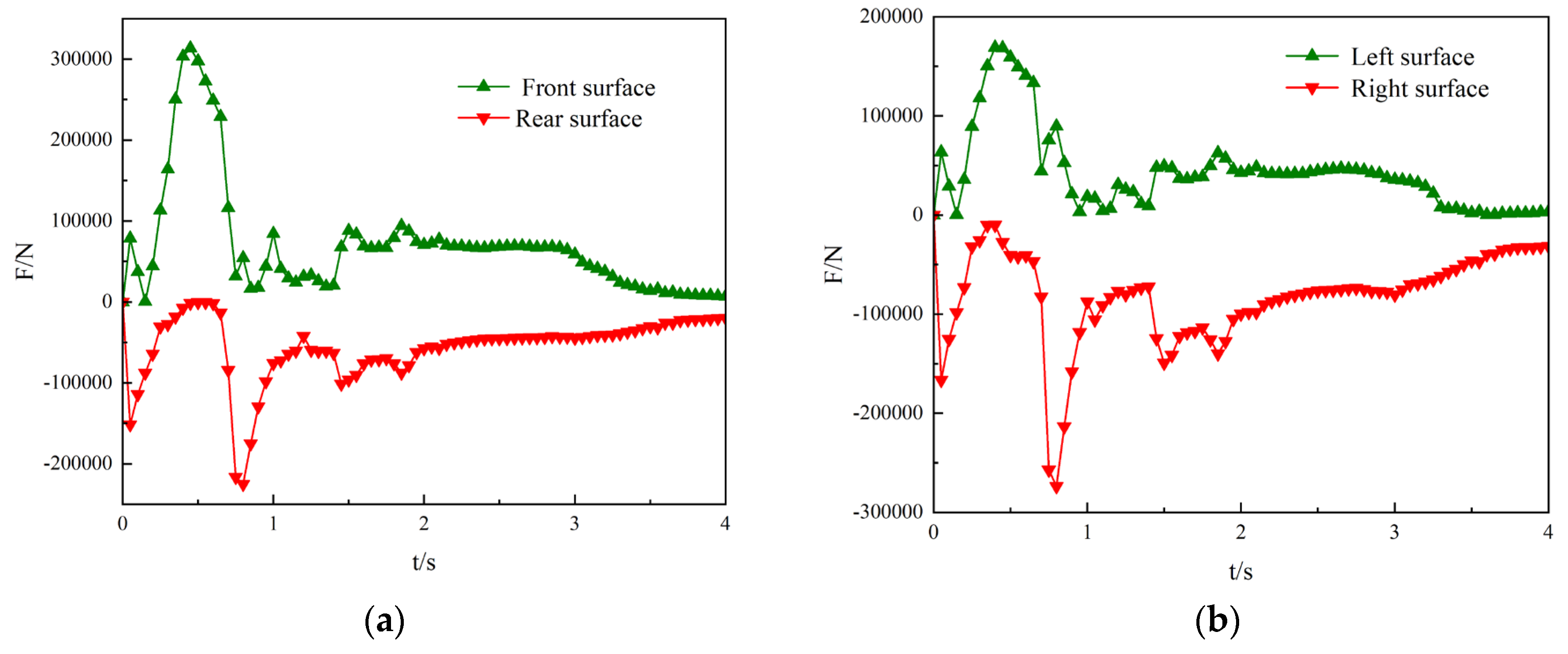
Under the combined braking and turning deceleration condition, the liquid cargo tank initially remains stationary. Unlike the straight-line deceleration, the ship’s velocity is decomposed into vectors, and during braking and turning, the vessel experiences acceleration in two perpendicular directions opposite to its initial velocity. Due to fluid inertia, this results in vigorous sloshing characterized by coupled movements in both directions. Taking a 50% fill rate as an example, at t = 0 s (Figure 11a), the fluid exhibits steady motion before braking begins. By t = 0.43 s, the inertia causes the fluid to impact the front bulkhead and the left wall simultaneously, as the fluid surges in two coupled directions. According to Figure 11, the impact force on the front bulkhead reaches its maximum at t = 0.43 s, with F_max = 317,323.42 N. The impact force on the left wall at the same time is 174,097.69 N. As evidenced in Figure 11b and Figure 12, the fluid tends to surge forward and to the side, but the front bulkhead and left wall impose constraints, forcing the fluid to move upward along these surfaces. Consequently, at t = 0.43 s, the combined volumetric force exerted by the fluid acts on both the front bulkhead and the left wall, producing the maximum coupled impact force.

Figure 11. Simulation results of fluid sloshing under braking and turning deceleration.

Figure 12. Variation of impact forces on the port and starboard walls of the liquid cargo tank over time. (a) Cloud plots of fluid sloshing at different time instances in the liquid cargo tank. (b) Variation of impact forces on the fore and aft bulkheads of the liquid cargo tank over time.

By t = 0.78 s, the fluid, impeded by the front bulkhead and sidewall, starts to flow backward toward the aft bulkhead, with the impact force on the aft bulkhead peaking at 234,500.98 N. Notably, the impact force on the front bulkhead remains larger than on the aft bulkhead throughout. Furthermore, the impact force on the right wall reaches a maximum of 283,550.54 N, with the impact on the right wall surpassing that on the left. The force curves demonstrate that early in deceleration, fluid movement is primarily along the direction toward the front bulkhead, making it the main impact target. As deceleration progresses, the dominant fluid velocity shifts toward the right wall, making it the primary impact surface in the later stage. Figure 11d–h shows that after the deceleration stops, and the fluid oscillates in a diagonal back-and-forth motion at its natural frequency until it gradually settles, illustrating complex coupled sloshing dynamics induced by combined directional accelerations.

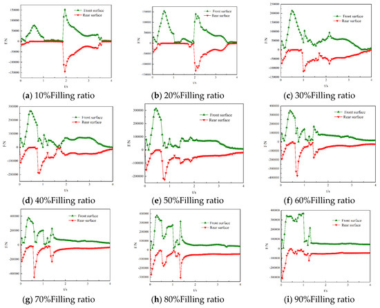
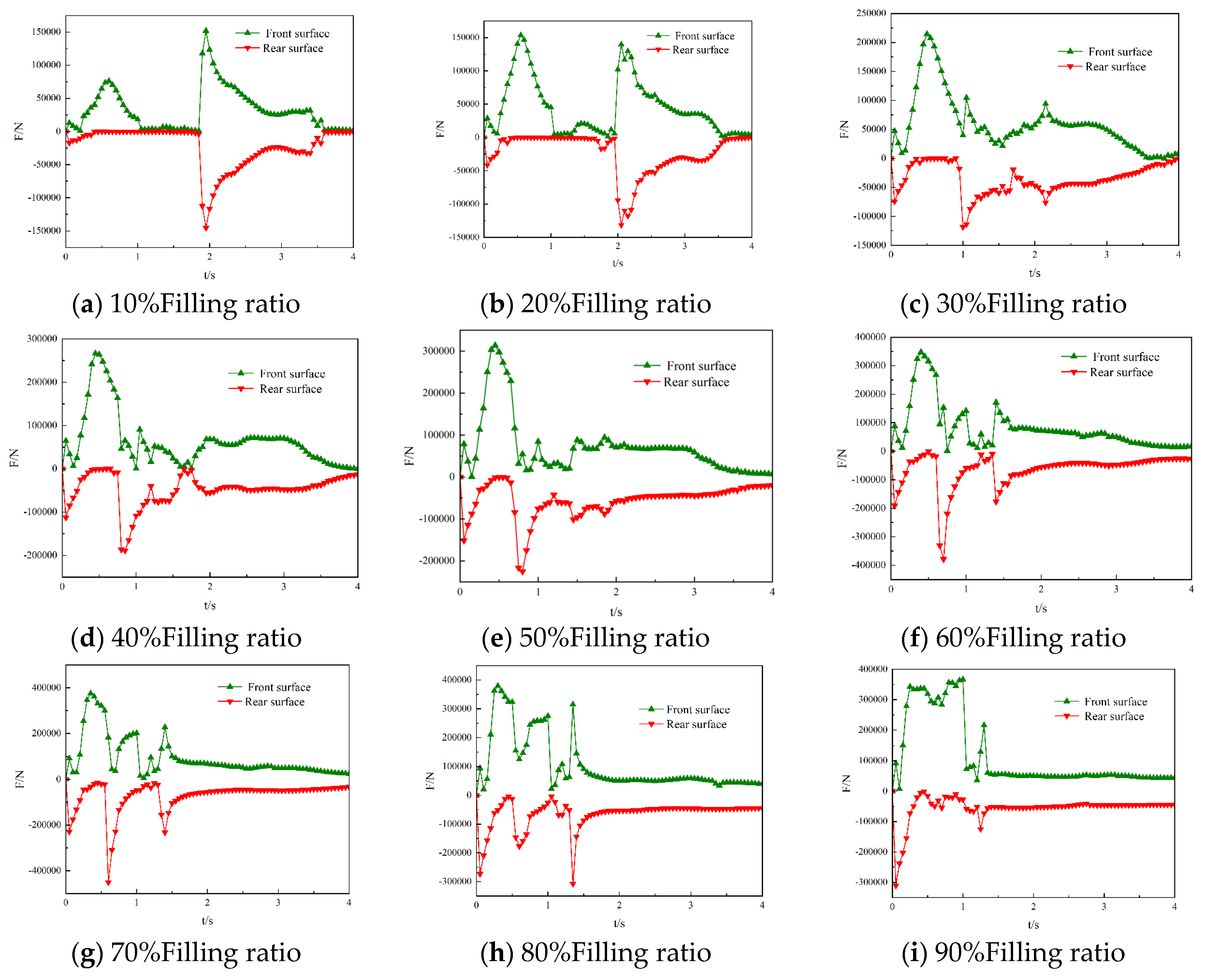
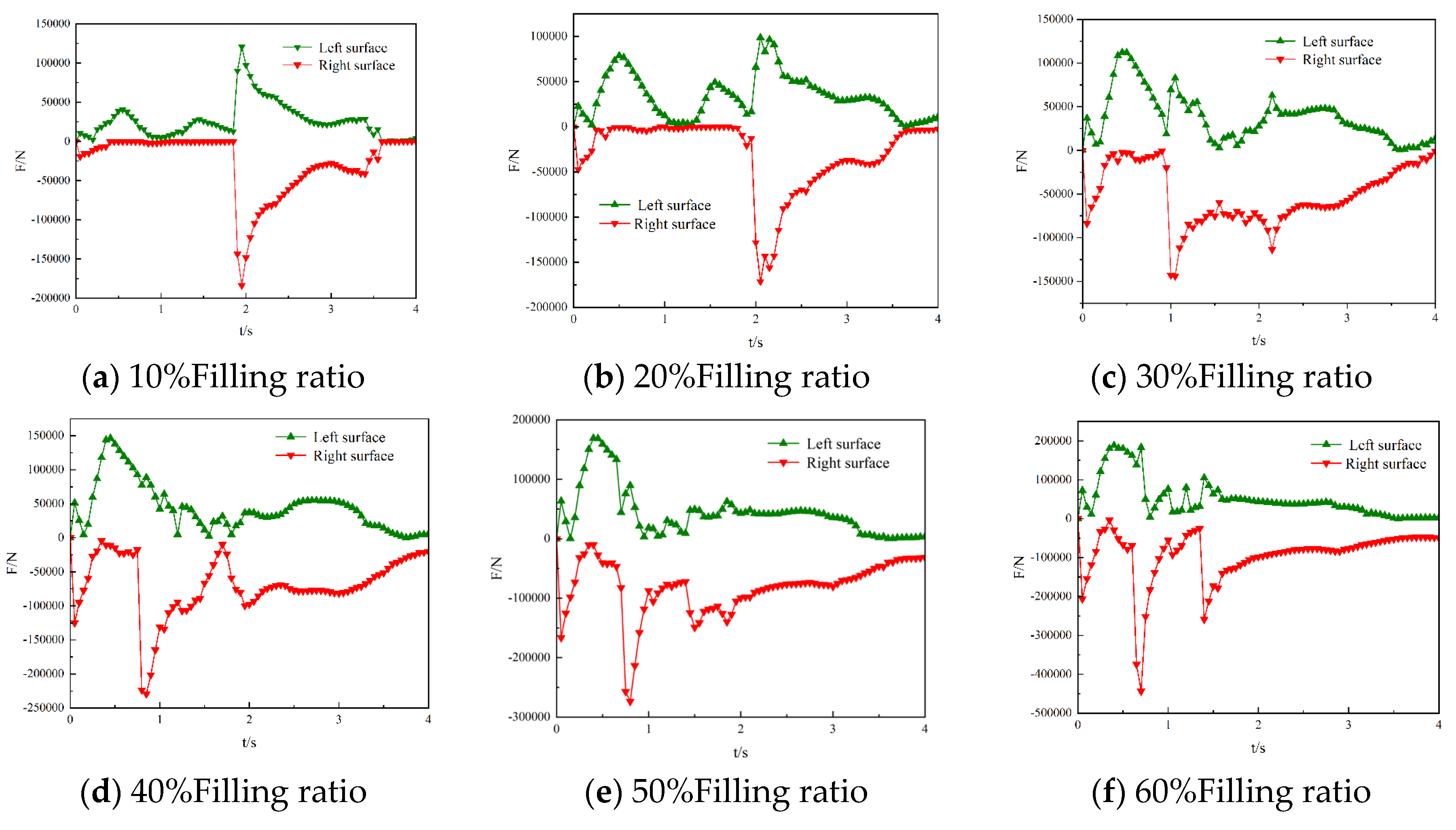
A control variable methodology was adopted, keeping all parameters constant except the liquid fill level, to evaluate the maximum impact force on the cargo tank across eight fill levels—10%, 20%, 30%, 40%, 60%, 70%, 80%, and 90%. Figure 13a–i present the impact force time histories on the fore and rear bulkheads, while Figure 14 shows the forces on the port and starboard walls.

Figure 13. Impact force curves on the front and rear bulkheads of the liquid cargo tank at the same filling ratio.

Figure 14. Impact force under different filling rates. (a) Maximum impact forces on the liquid cargo tank at different filling ratios. (b) Time of maximum impact force occurrence at different filling ratios.

Results on the front and rear bulkheads indicate that impact forces on the fore and aft bulkheads exhibit a double-peak pattern at 60%, 70%, and 80% fill levels, reflecting intensified sloshing. Specifically, impact force on the fore bulkhead initially increases with fill level, peaking at 80%, then gradually decreases but remains above zero due to continued volumetric effects. This trend confirms that increasing liquid volume up to 80% correlates with higher impact forces; beyond this, the larger liquid volume reduces free sloshing space, stabilizing the fluid motion.

The occurrence time of the maximum impact force on the fore bulkhead shortens with increasing fill level, decreasing from 0.59 s at lower fill levels to 0.25 s at higher levels. Compared to the linear deceleration case, the peak impact occurs later, indicating greater fluid freedom to move, which extends the time to reach maximum impact. In the fore-bulkhead direction, the braking–turn condition yields similar conclusions to the linear case; however, the maximum impact force is lower because the volumetric force exerted by the liquid on the fore bulkhead is partial rather than fully continuous.

Results on the port and starboard walls also exhibit a double-peak pattern. Similarly, at filling levels of 70%, 80%, and 90%, a “double-peak” phenomenon is observed near the maximum impact force, indicative of complex sloshing dynamics.

As shown in Figure 15 and Figure 16, under the braking–turn condition, the impact force on the port wall initially increases with higher filling ratios. The timing of the maximum impact force on the port wall shifts with increasing fill levels, decreasing from 0.54 s at lower fill ratios to 0.38 s near 70%, and then increasing to 0.88 s at the highest fill ratios. Before reaching 70% fill, the maximum impact force on the port wall occurs prior to the fluid surge, with the entire volumetric force exerted on both the front bulkhead and the port wall due to inertia effects. Beyond the 70% fill level, the peak impact on the port wall occurs during the fluid’s oblique oscillation inside the tank. At these higher fill ratios, the sloshing motion persists throughout the 1 s deceleration period, causing multiple impacts on the port wall as the fluid repeatedly strikes the surface. This behavior is due to the increased volume of fluid capable of impacting the wall, emphasizing that higher fill levels enhance the potential severity of impact forces during deceleration maneuvers.

Figure 15. Impact force curves on the port and starboard walls of the liquid cargo tank at different filling ratios.

Figure 16. Impact forces at different filling ratios. (a) Maximum impact forces on the liquid cargo tank at different filling ratios. (b) Time of occurrence of maximum impact forces at different filling ratios.

4.3. Influence of Fluid Sloshing on BOG Generation in the Liquid Cargo Tank

During LNG transportation, the filling ratio of the liquid cargo tank is typically maximized to improve economic efficiency. Given the complex heat exchange mechanisms and increased impact forces observed at an 80% fill level, this section focuses on an in-depth analysis of the B-type liquid cargo tank operating at 80% capacity.

4.3.1. Linear Deceleration Scenario

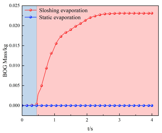
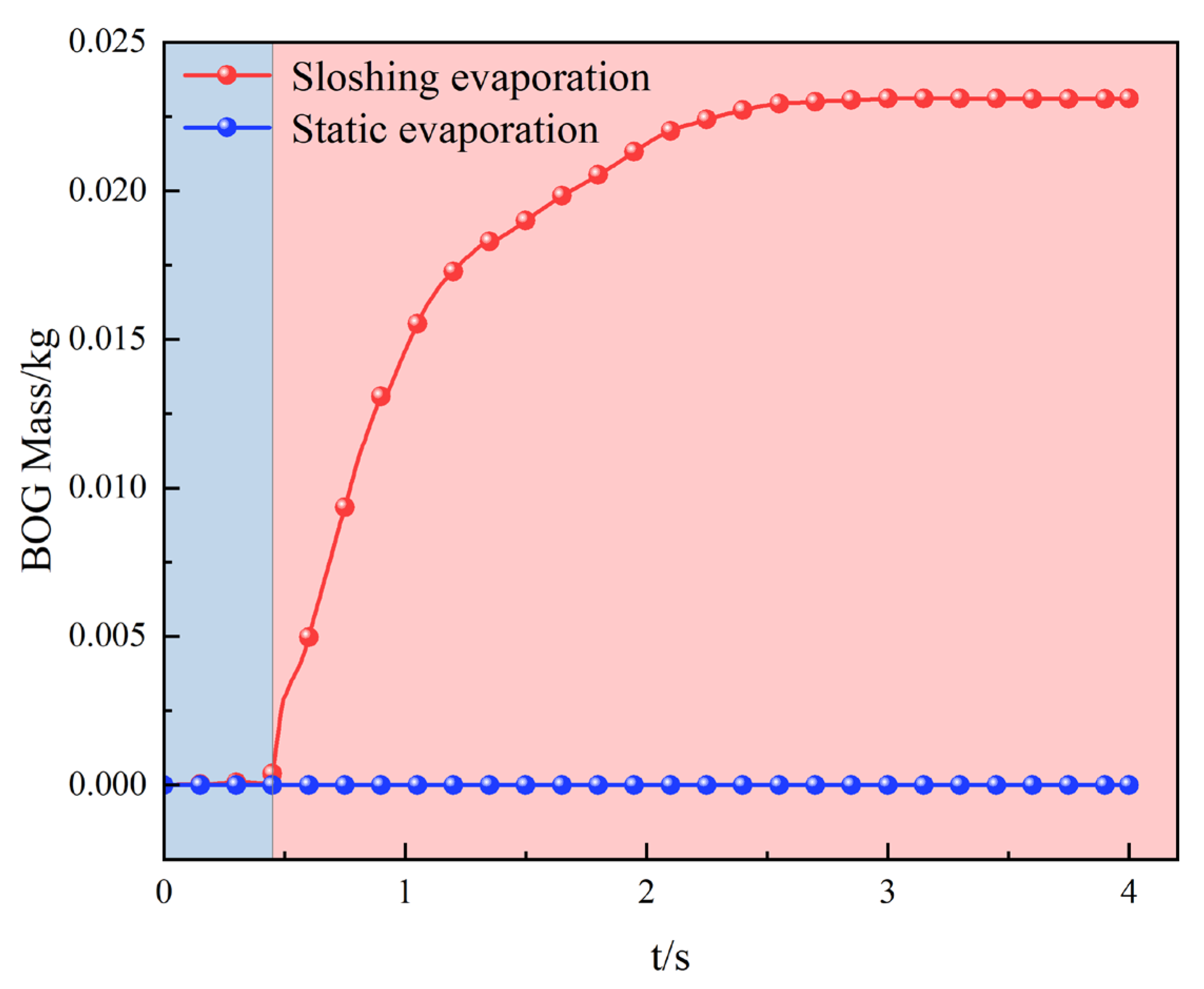
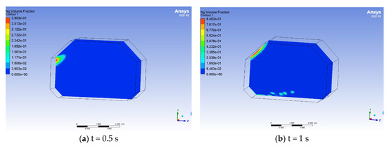
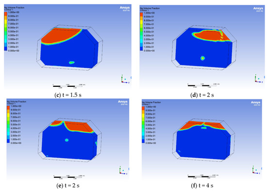
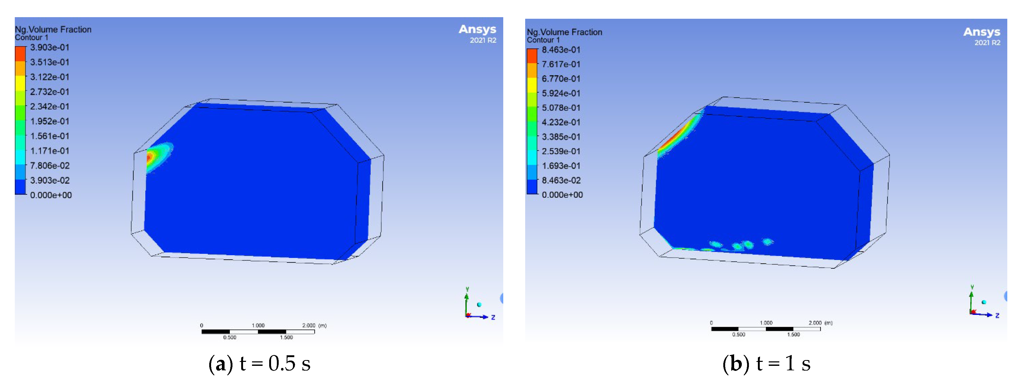
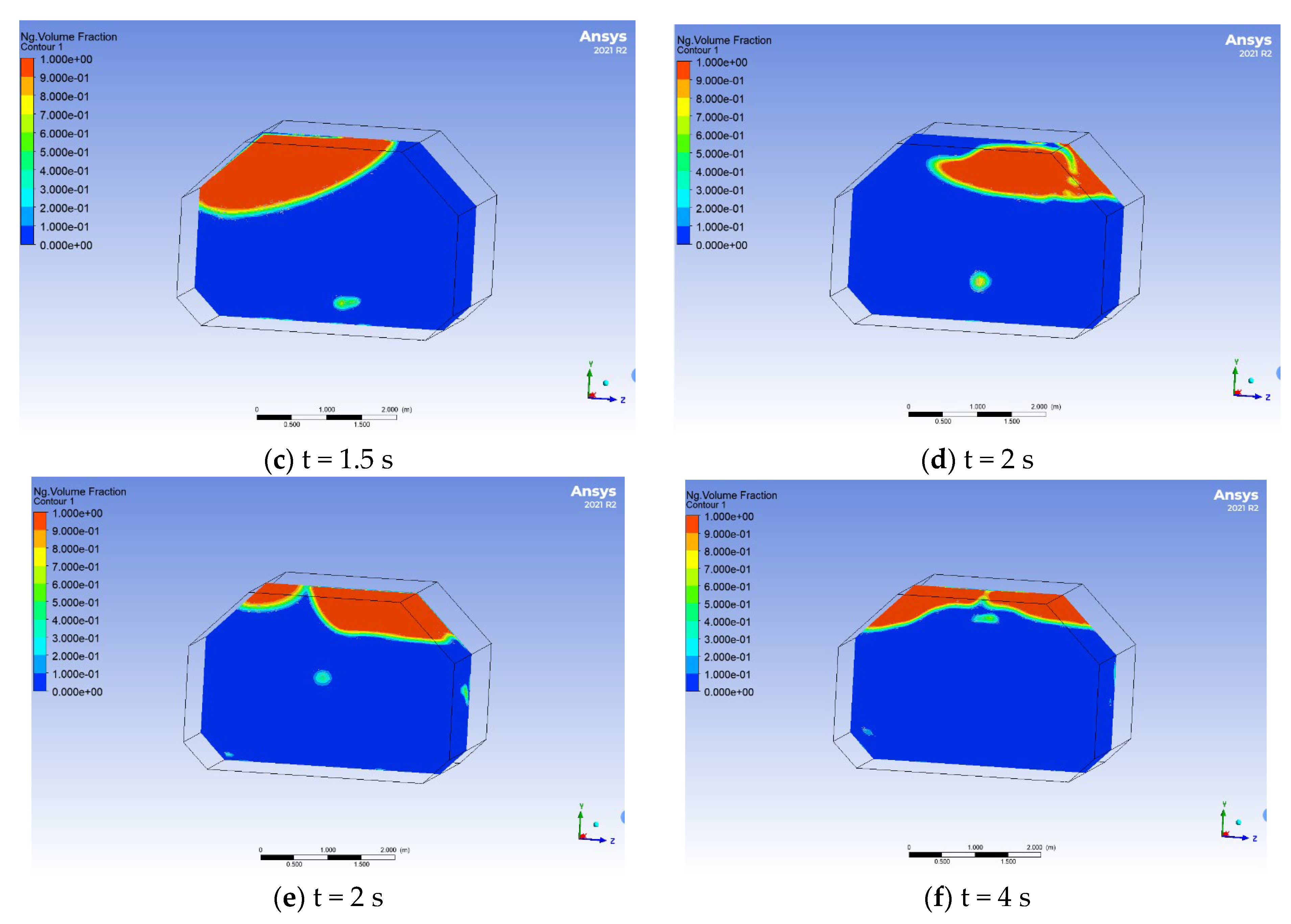
Figure 17 and Figure 18 present cloud plots of the gas–liquid phase distribution along the central longitudinal section of the cargo tank during the sloshing process. Prior to 0.5 s, as shown in Figure 17a,b, the gas–liquid interface remains stable with a standing-wave pattern, and BOG production remains negligible. After 0.5 s, linear deceleration triggers liquid overturning within the tank’s geometry. Due to the vertical placement of the top and side walls, the liquid impacts the aft bulkhead, and part of the overturning liquid forms jets, fragmenting the gas–liquid interface. During this phase, intensified sloshing enhances heat transfer between the liquid and tank walls; impacts increase the liquid surface area exposed to high-temperature vapor, leading to a rapid rise in BOG generation. When deceleration ends at 1 s, the tank becomes stationary, and the liquid, no longer externally driven, oscillates at its natural frequency with diminishing amplitude. This oscillation gradually reduces BOG production. Beyond 2.5 s, the fluid motion stabilizes, and natural vapor convection dominates the phase behavior within the tank.

Figure 17. Cloud plots of gas–liquid phase distribution inside the liquid cargo tank at different time instances under an 80% filling ratio.

Figure 18. BOG generation in the liquid cargo tank during linear deceleration braking conditions.

4.3.2. Ship Deceleration and Turning Maneuver

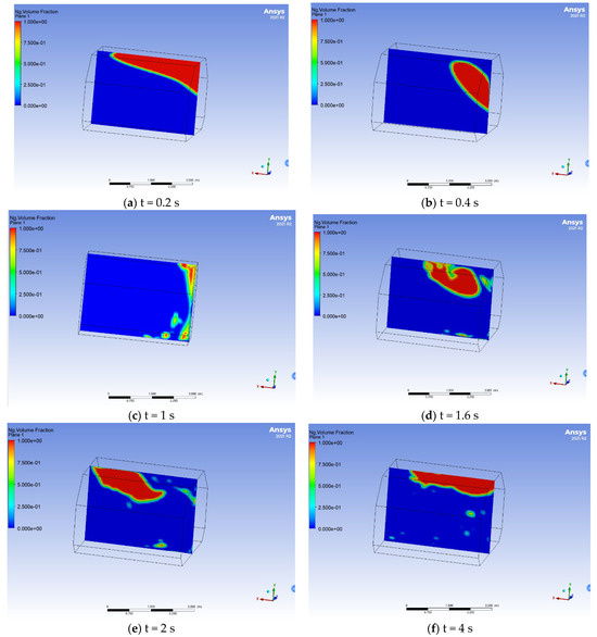
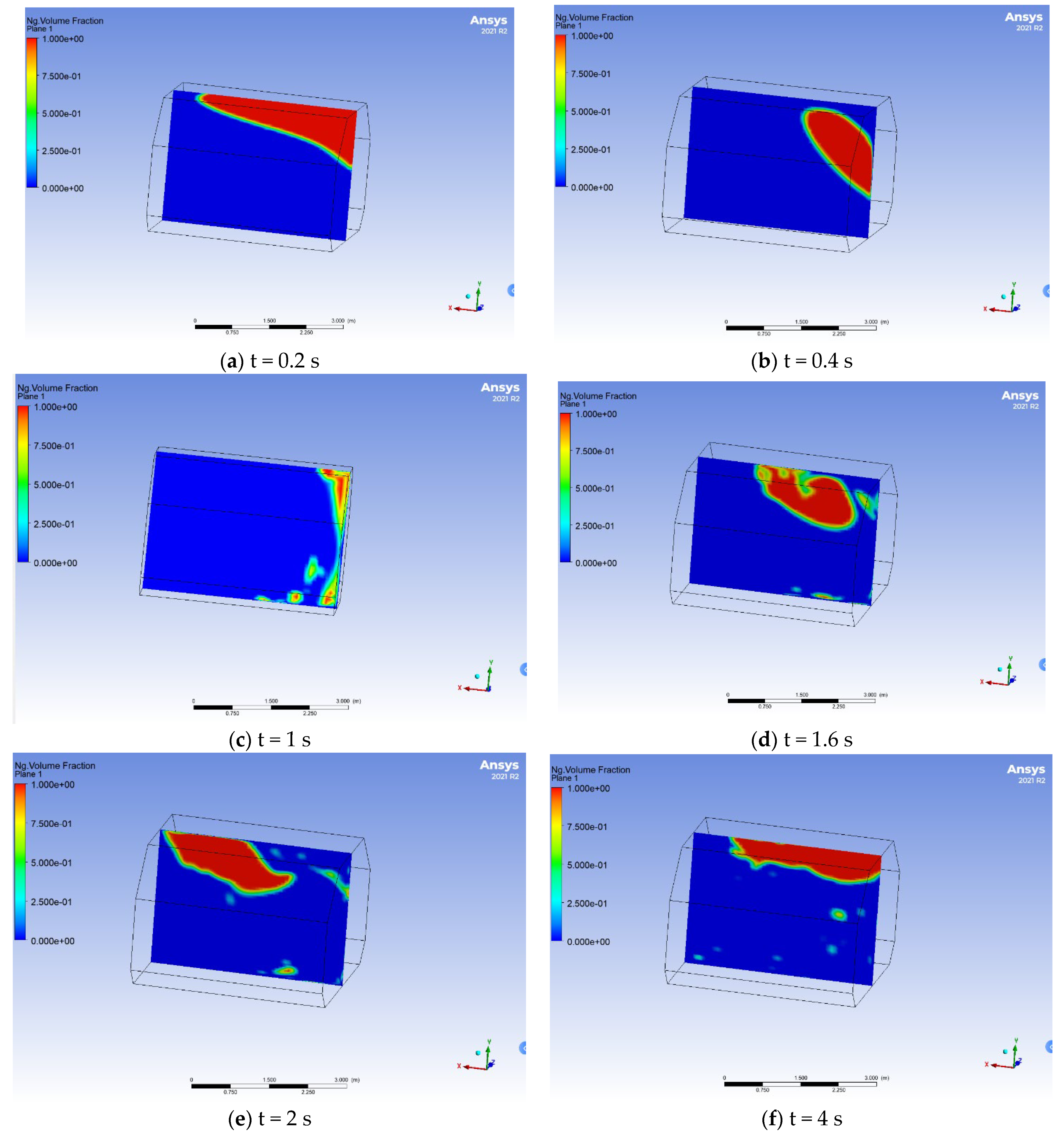
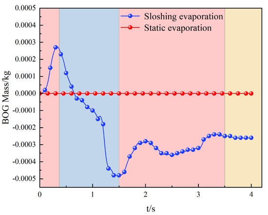
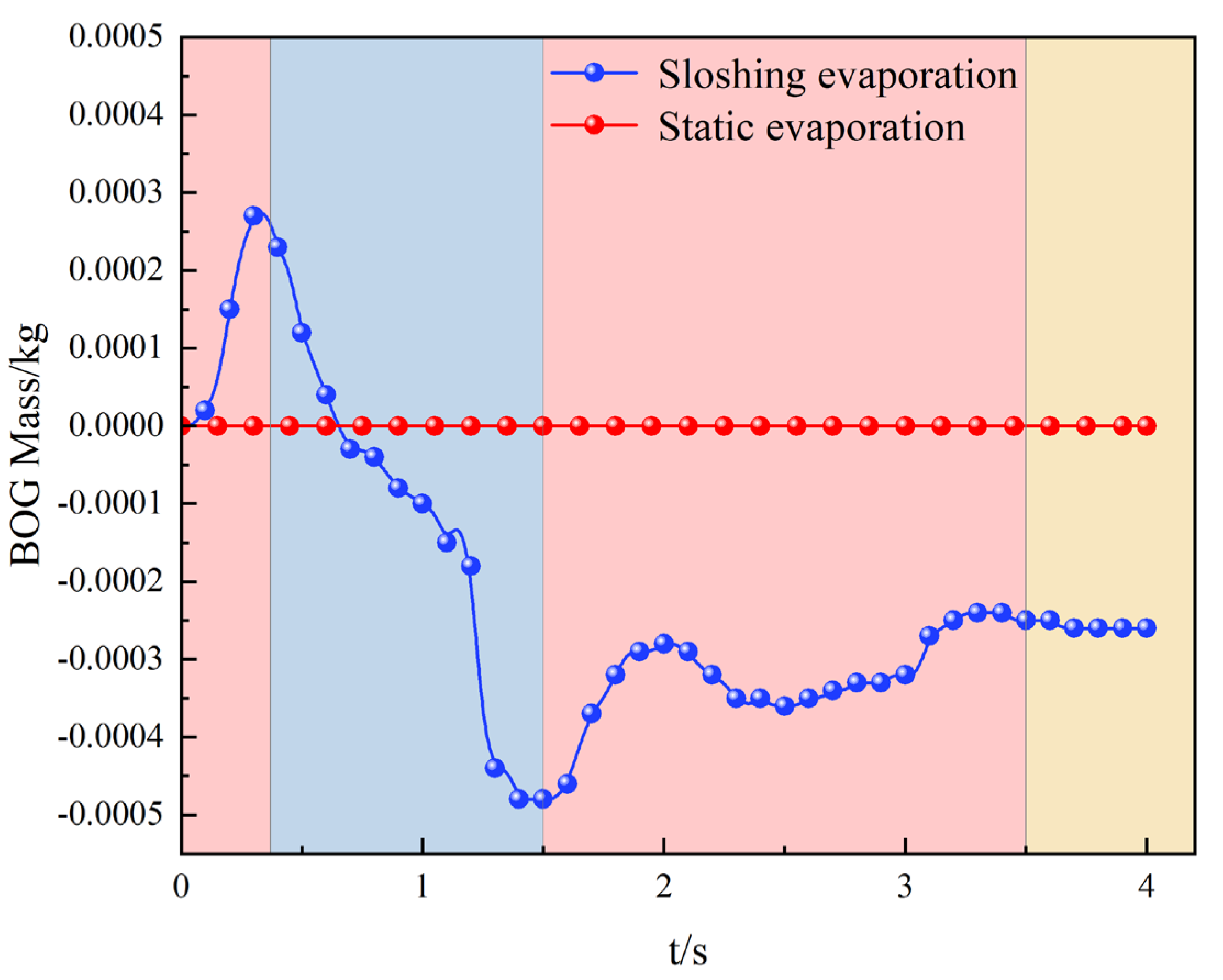
Figure 19 displays cloud plots of the gas–liquid phase distribution along the central longitudinal section of the cargo tank during sloshing. Figure 20 illustrates the BOG (boil-off gas) generation over 4 s under conditions of ship deceleration and turning. During this interval, the gas mass exhibits a characteristic “increase–decrease–increase” pattern, arising from coupled effects of inertial forces and multiphase nonequilibrium thermodynamics. Initially, rapid deceleration sharply increases the liquid-phase kinetic energy, destabilizing the gas–liquid interface and inducing vortex entrainment. These vortices promote localized evaporation fluxes, leading to a rapid rise in gas mass. As the liquid kinetic energy dissipates, pressure oscillations generate transient low-pressure zones, facilitating flash evaporation. Simultaneously, microscale turbulent mixing enhances liquid–gas contact, increasing condensation nucleation rates and reducing the gas mass. Subsequently, heat flux from the external environment gradually infiltrates through boundaries with low heat transfer coefficients, reconstructing the thermal boundary layer and producing a temperature polarization effect. This sustained thermal imbalance drives continuous evaporation at the liquid film surface, ultimately reversing phase change dynamics and causing a later-stage increase in gas mass.

Figure 19. Cloud plots of internal gas–liquid phase distribution in the cargo tank at 80% filling ratio during sloshing at different time instances.

Figure 20. Boil-off gas (BOG) generation in the cargo tank during the ship’s deceleration and turning maneuver.

Compared to static evaporation, sloshing driven by ship deceleration and turning enhances heat transfer between the fluid and the surrounding vapor before 0.4 s. After this point, the improved contact facilitates condensation, reducing BOG generation. From 1.5 to 3 s, liquid oscillation becomes the dominant mechanism, with evaporation chiefly driving mass increases. Beyond 3 s, the system gradually transitions back to static evaporation conditions, and the BOG variation rate aligns with that observed under static conditions.

4.3.3. Longitudinal Ship Motion (Pitching)

(a)

Effect of Different Sloshing Periods

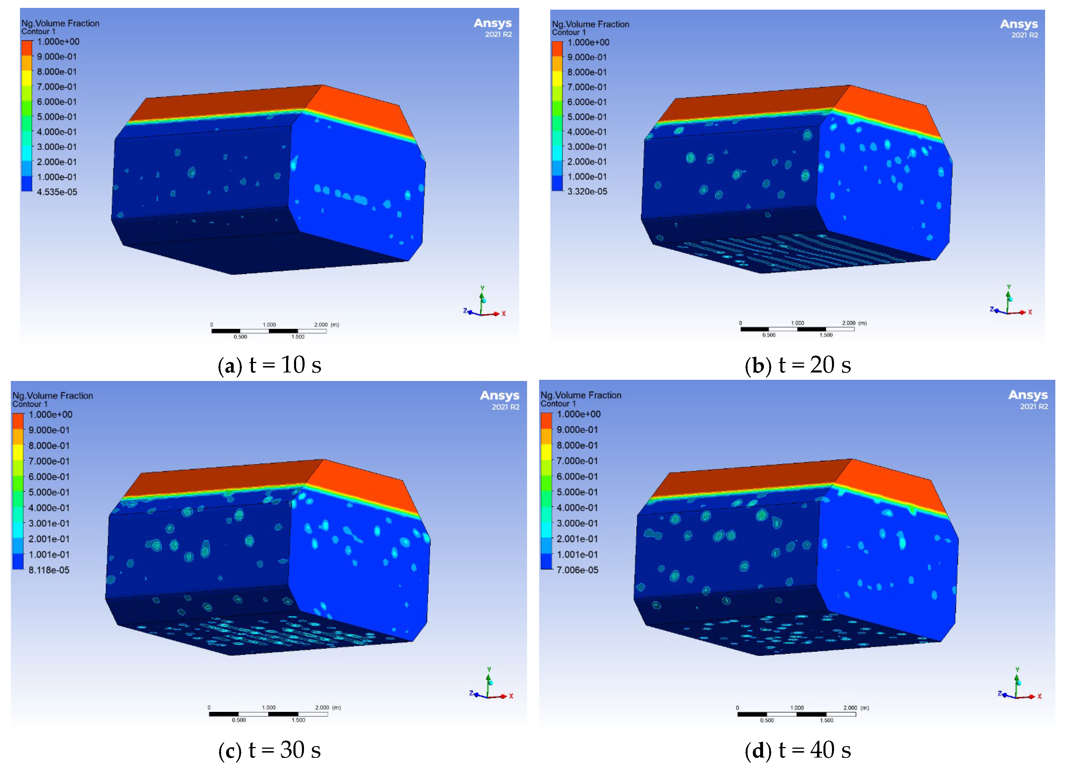
Figure 21, Figure 22 and Figure 23 present cloud plots of the gas–liquid phase distribution within the cargo tank during longitudinal ship motion, with a sloshing amplitude of 0.03 m and pitching periods of 2.27 s, 3 s, and 4 s, respectively. Compared to static conditions, a greater number of bubbles are observed on the tank walls under sloshing, with many forming earlier at the tank bottom. This suggests that sloshing enhances heat transfer at this location and promotes forced convective heat exchange between the LNG and tank walls. The vigorous liquid motion and mixing induced by sloshing generate forced convection, effectively transferring heat from the tank walls into the LNG, accelerating heat propagation, and increasing the overall heat flux into the liquid phase. Additionally, tank inclination caused by sloshing enlarges the contact surface between LNG and the wall, further facilitating heat ingress. Collectively, these effects strengthen heat transfer mechanisms and contribute to higher BOG generation during ship motion.

Figure 21. Gas–liquid phase distribution cloud plots of the cargo tank at different time instants during sloshing with a period of 2.27 s.

Figure 22. Gas–liquid phase distribution cloud plots of the cargo tank at different time instants during sloshing with a period of 3 s.

Figure 23. Gas–liquid phase distribution cloud plots of the cargo tank at different time instants during sloshing with a period of 4 s.

At a period of 2.27 s, corresponding to the natural sloshing frequency of the cargo tank at 80% fill, resonance effects induce more vigorous fluid motion compared to periods of 3 s and 4 s. Figure 24 and Figure 25 illustrate the gas–liquid phase distribution along the central longitudinal plane, revealing dynamic behaviors of the free surface. Under the 2.27 s period, the gas–liquid interface becomes highly fragmented, with liquid droplets exhibiting hydraulic jump phenomena. A relaxation period of 10 s precedes the onset of steady-state evaporation. These behaviors significantly enhance heat transfer, resulting in a higher bubble count at 10 s relative to the 3 s and 4 s cases. By 20 s, bubbles form earlier and are more densely distributed at the tank bottom. In addition to resonance effects, heat transfer at 3 s exceeds that at 4 s; specifically, more bubbles are generated at 10 s, and by 20 s, the bubbles on the tank bottom are more numerous and concentrated, rapidly stabilizing the evaporation process. These findings confirm that resonance amplifies sloshing-induced heat transfer and BOG production, with the optimal effect occurring near the natural sloshing period.

Figure 24. Gas–liquid phase distribution contours of the cargo tank at different time instants during sloshing with a period of 2.27 s.

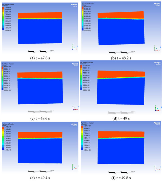
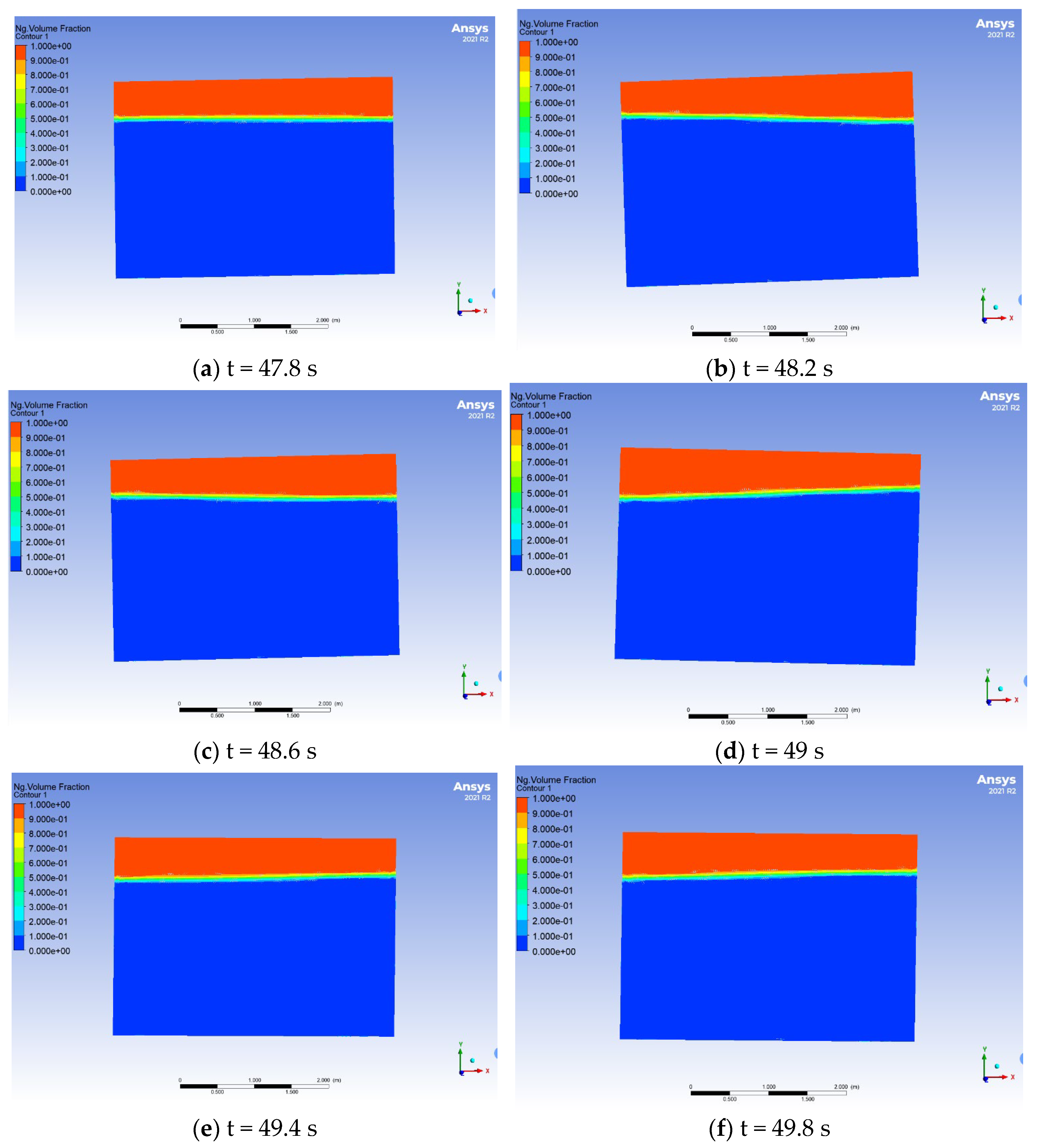
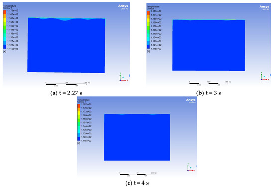
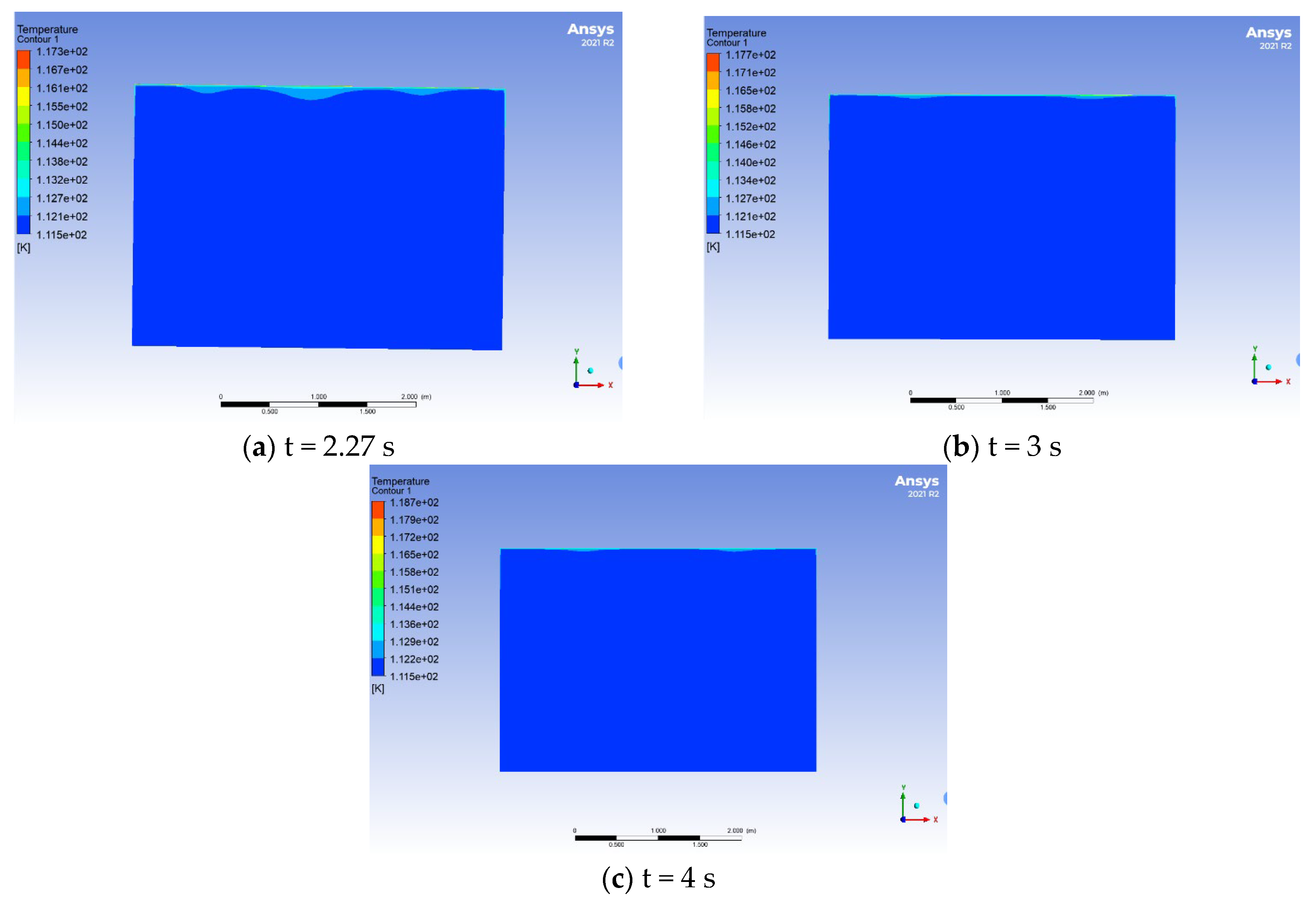
Figure 25. Temperature distribution contours on the longitudinal central section of the cargo tank at 48 s under different sloshing periods.

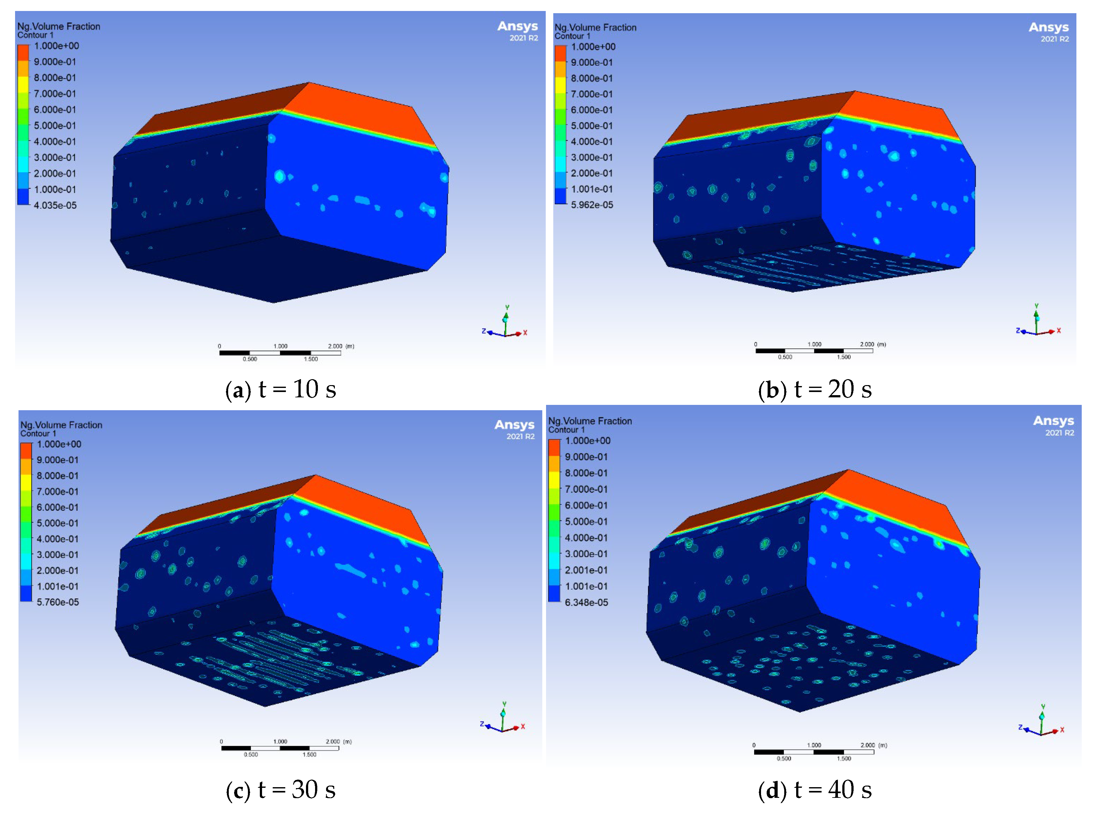
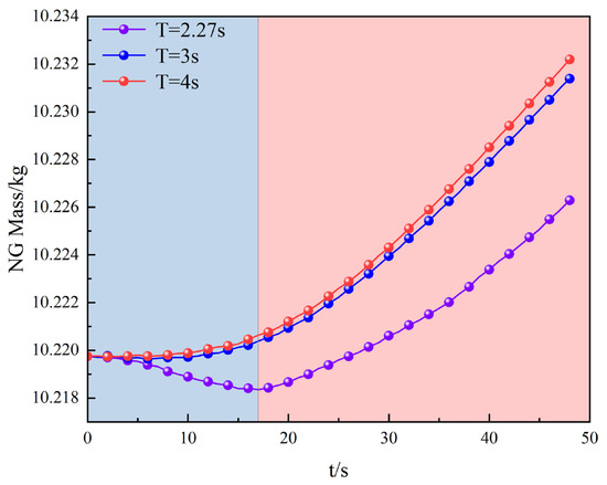
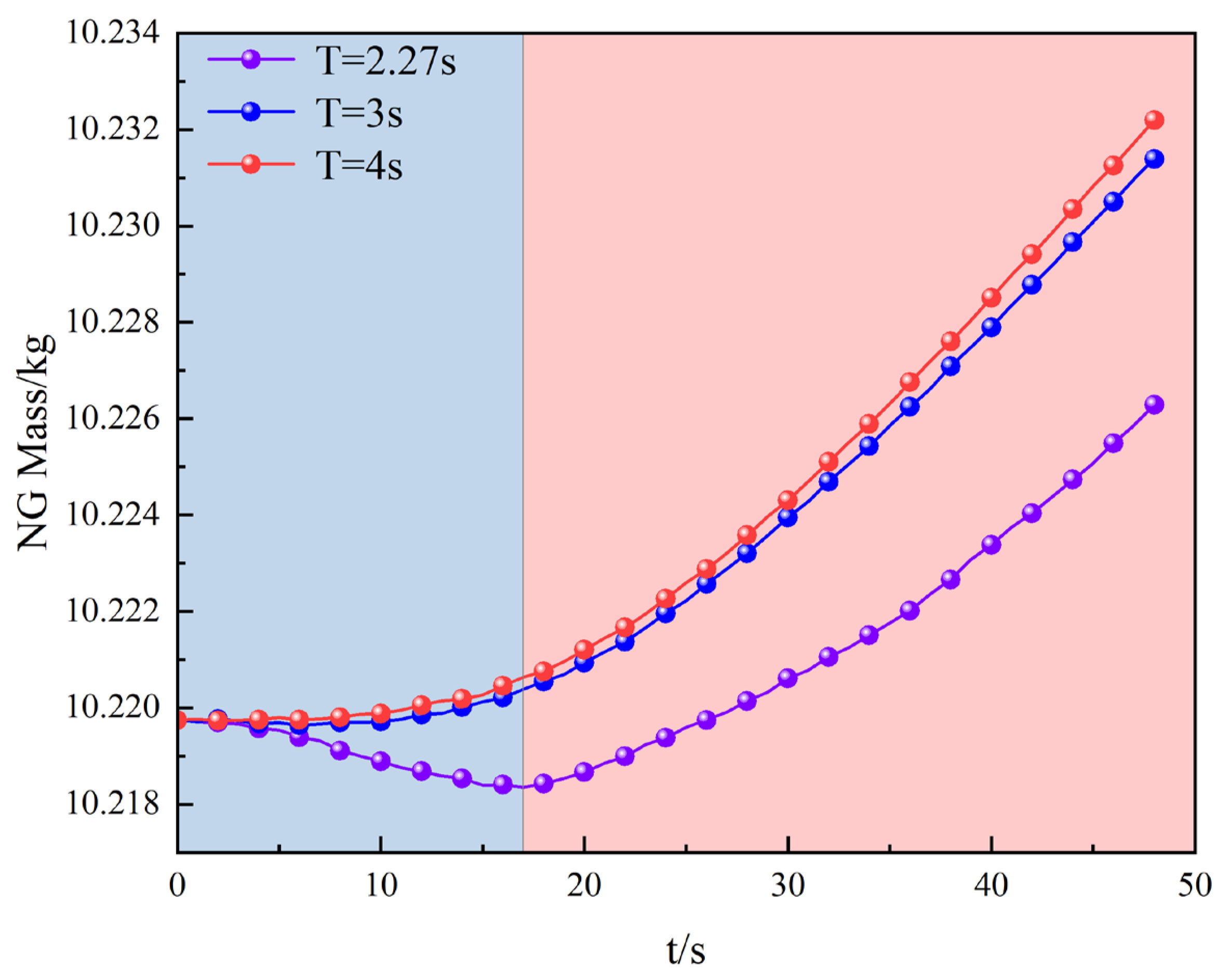
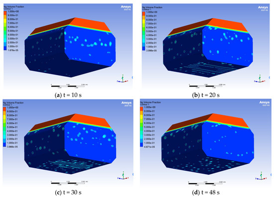
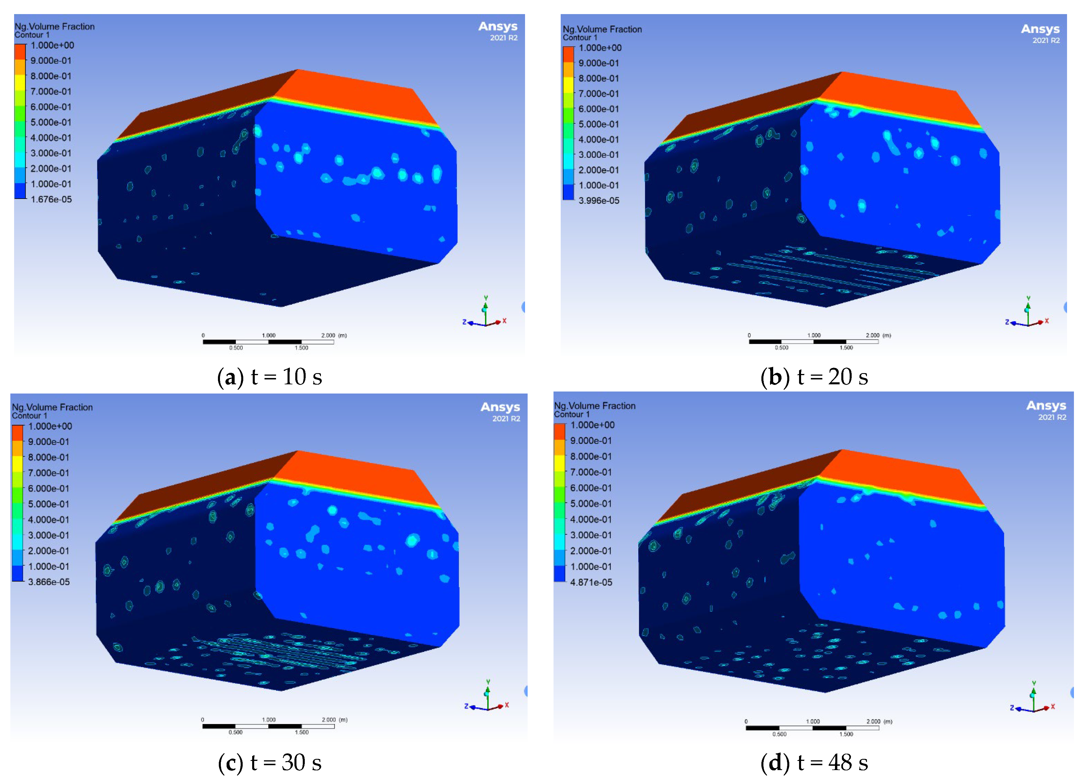
Figure 26 depicts the variation of the NG volume within the cargo tank over 0–48 s under different sloshing periods. As observed in Figure 27, Figure 28 and Figure 29, decreasing the sloshing period results in an increased number of BOG bubbles on the tank walls at any given time. However, in Figure 27, the overall NG mass in the cargo tank decreases as the sloshing period shortens. Specifically, for the 2.27 s period, the NG mass declines during the initial 0–16 s. This counterintuitive behavior arises because resonant sloshing induces vigorous interfacial disturbances, which significantly increase the gas–liquid contact area, thereby promoting condensation nucleation. At the same time, local pressure fluctuations elevate the instantaneous saturation temperature, suppressing interfacial evaporation. Additionally, transient heat transfer between the tank wall and the fluid creates a temperature gradient near the wall, while microscale turbulence generated during the early energy dissipation enhances heat transfer from the gas to the liquid phase, leading to partial unsteady condensation. As external heat input persists, the system approaches thermodynamic equilibrium, kinetic energy of the fluid dissipates, and evaporation begins to dominate. This causes the net phase change to shift toward gradual net evaporation, resulting in an increase in gas mass. Among the three cases, the 4 s period yields the highest NG mass, with minimal condensation at the gas–liquid interface, and the maximum retention of BOG generated by sloshing.

Figure 26. BOG generation over time in the cargo tank under different sloshing periods.

Figure 27. Gas–liquid phase distribution contours of the cargo tank at different time instants under a sloshing amplitude of 0.05 m.

Figure 28. Gas–liquid phase distribution contours of the cargo tank at different time instants under a sloshing amplitude of 0.07 m.

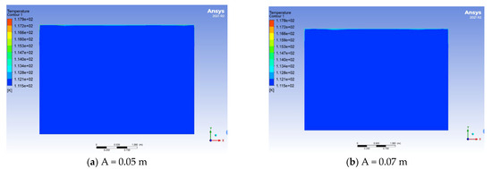
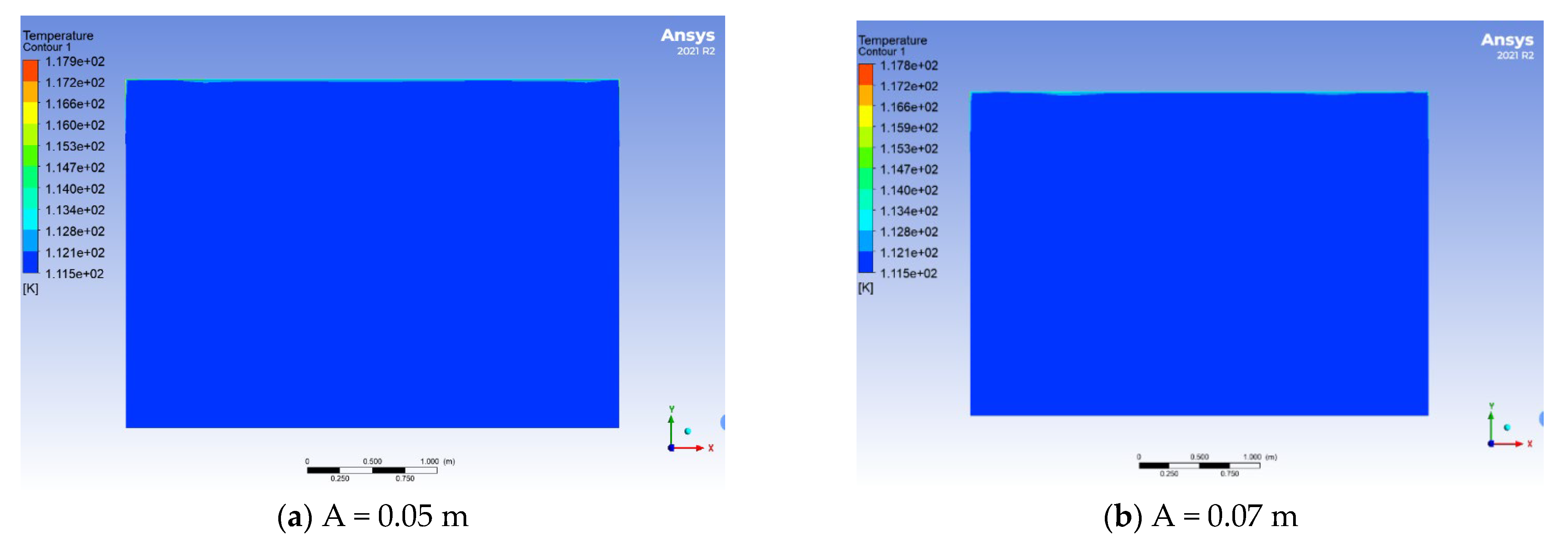
Figure 29. Temperature distribution contours of the cargo tank at 48 s under different sloshing amplitudes.

(b)

Influence of different sloshing amplitudes

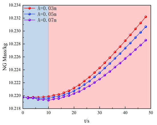
In this subsection, the sloshing period of the cargo tank is fixed at 4 s, and the impact of different sloshing amplitudes—0.03 m, 0.05 m, and 0.07 m—on BOG generation is analyzed. The case with a 4 s period and 0.03 m amplitude has been detailed in the previous subsection. Figure 28 and Figure 29 present the gas–liquid phase distribution contours inside the cargo tank over 48 s of evaporation for amplitudes of 0.05 m and 0.07 m, respectively. Consistent with prior findings, more vigorous sloshing results in increased bubble formation on the tank walls. This indicates that higher sloshing amplitudes facilitate greater absorption of external energy, thus promoting faster bubble nucleation and growth on the tank surfaces. Additionally, Figure 30 displays the temperature distribution contours along the central cross-section, revealing a broader high-temperature region at the 0.07 m amplitude. These observations suggest that larger sloshing amplitudes intensify heat transfer interactions and influence the thermal and phase-change dynamics within the cargo tank, ultimately affecting BOG generation rates.

Figure 30. NG generation in the cargo tank at different sloshing amplitudes over time.

Figure 30 depicts the temporal evolution of NG mass within the cargo tank for varying sloshing amplitudes. As the amplitude increases from 0.03 m to 0.07 m, the NG mass inside the tank decreases overall. For the amplitudes of 0.05 m and 0.07 m, the NG mass initially declines, then begins to increase at later times. The intensified sloshing promotes vigorous gas–liquid mixing, which enhances condensation at the gas–liquid interface and suppresses net BOG generation. This indicates that larger sloshing amplitudes can effectively mitigate BOG accumulation by increasing heat exchange and promoting phase change processes that favor condensation over evaporation.

Under longitudinal pitching conditions, it is observed that during the initial stage of sloshing, the vigorous movement markedly increases energy absorption from the external environment, leading to the formation of numerous vapor bubbles along the cargo tank walls. However, the overall temperature distribution within the tank remains relatively unchanged; only localized temperature variations occur near the gas–liquid interface and the tank walls. The intensified mixing caused by sloshing enhances condensation at the interface, resulting in simultaneous evaporation and condensation processes. As a result, the net NG content inside the tank does not increase as expected; instead, more intense sloshing actually reduces the total NG mass in the tank. This indicates that the dynamic mixing promotes phase change mechanisms that favor condensation, ultimately suppressing overall BOG accumulation despite increased heat transfer activity.

5. Conclusions

This study employed the Volume of Fluid (VOF) method to simulate sloshing and phase-change phenomena in a Type-B LNG cargo tank during emergency stop conditions. Key findings are summarized as follows:

(1)

This study proposes a physical mechanism of the BOG rise–fall–rise pattern. The core mechanism is the coupled interplay between inertial forces and non-equilibrium thermodynamics, where rapid deceleration induces transient turbulence and vortex entrainment, enhancing local evaporation flux and causing initial gas mass rise. The subsequent dissipation of liquid energy and pressure oscillations promote condensation, while external heat flux gradually re-establishes thermal boundary layers, driving sustained evaporation and reversing phase change dynamics. Flow disturbance caused by vessel rolling increases BOG generation fluctuations by approximately 35%. This model’s predictions offer a quantitative basis for dynamic tank pressure control strategies to enhance safety and efficiency.

(2)

Static Evaporation: At 80% fill, high-temperature gas initially accumulates at the tank corners, migrating toward the center and forming an “X-shaped” temperature distribution. BOG forms first at the tank bottom corners and later along the periphery, with higher fill levels increasing heat absorption and BOG production (≈0.0009 kg/100 s).

(3)

Straight-line Deceleration: During deceleration, impact forces on the front bulkhead peak at 80% fill (~462,209 N), with impact timing accelerating as fill increases (from 0.57 s at 10% to 0.21 s at 90%). Sloshing impacts both the front bulkhead and port wall, with impact force peaks following a rise–fall–rise pattern driven by impact magnitude and heat transfer mechanisms. Notably, impact forces are maximized at specific fill ratios and impact times, with early sloshing enhancing heat transfer, while later oscillations promote condensation, reducing BOG. Impact force magnitude on the port wall increases with fill ratio, with rapid impacts occurring in initial stages due to high energy fluid motion.

(4)

Impact of Sloshing Dynamics: Sloshing substantially enhances heat transfer, especially within the first 2.2 s, causing sharp BOG increases. Post-2.2 s, stabilized motion and natural convection diminish BOG generation rates. Braking with turning intensifies both heat transfer and condensation, producing a rise–fall–rise BOG pattern. Early impacts (before 0.4 s) increase transfer, subsequent condensation reduces BOG, oscillations from 1.5–3 s favor evaporation, raising BOG again, beyond 3 s static evaporation dominates.

(5)

Longitudinal Pitching: Initial intense sloshing boosts energy absorption and vapor bubble formation, with minor temperature distribution changes limited mostly near gas interfaces. Sloshing enhances mixing and condensation, preventing NG content from reaching equilibrium levels, higher sloshing amplitudes correspond to lower NG content.

References

- He, D.B.; Jia, C.Y.; Wei, Y.S.; Guo, J.L.; Ji, G.; Li, Y.L. Current situation and development trend of world natural gas industry. Nat. Gas Ind. 2022, 42, 1–12. [Google Scholar]
- Li, C.; Zhao, Z.; Ding, J.; Liu, X.; Pu, X. Numerical study of thermodynamic and hydrodynamics in a type B LNG cargo tank during sloshing excitation. Appl. Therm. Eng. 2024, 247, 123048. [Google Scholar] [CrossRef] [Scilit]
- Muttaqie, T.; Sasmito, C.; Kadir, A. Structural Strength Assessment of 20-ft LNG ISO Tank: An Investigation of Finite Element Analysis and ASME Design Guidance. IOP Conf. Ser. Earth Environ. Sci. 2022, 972, 012015. [Google Scholar] [CrossRef] [Scilit]
- Chong, W.; Hongde, Q.; Ge, L.; Ting, G. Study on sloshing of liquid tank in large LNG-FSRU based on CLSVOF method. Int. J. Heat Technol. 2016, 34, 616–622. [Google Scholar] [CrossRef] [Scilit]
- Lee, S.J.; Kim, M.H.; Lee, D.H.; Kim, J.W.; Kim, Y.H. The effects of LNG-tank sloshing on the global motions of LNG carriers. Ocean. Eng. 2007, 34, 10–20. [Google Scholar] [CrossRef] [Scilit]
- Miana, M.; Legorburo, R.; Díez, D.; Hwang, Y.H. Calculation of boil-off rate of liquefied natural gas in mark III tanks of ship carriers by numerical analysis. Appl. Therm. Eng. 2016, 93, 279–296. [Google Scholar] [CrossRef] [Scilit]
- Lin, Y.; Ye, C.; Yu, Y.; Bi, S.W. An approach to estimating the boil-off rate of LNG in type C independent tank for floating storage and regasification unit under different filling ratio. Appl. Therm. Eng. 2018, 135, 463–471. [Google Scholar] [CrossRef] [Scilit]
- Zakaria, M.S.; Osman, K.; Saadun, M.N.A.; Manaf, M.Z.A.; Hanafi, M.H.M. Computational simulation of boil-off gas formation inside liquefied natural gas tank using evaporation model in ANSYS fluent. Appl. Mech. Mater. 2013, 393, 839–844. [Google Scholar] [CrossRef] [Scilit]
- Zakaria, M.S.; Osman, K.; Musa, M.N. Boil-off gas formation inside large scale liquefied natural gas (lng) tank based on specific parameters. Appl. Mech. Mater. 2012, 229, 690–694. [Google Scholar] [CrossRef] [Scilit]
- Zakaria, M.S.; Osman, K.; Yusof, A.A.; Hanafi, M.H.M.; Saadun, M.N.A.; Manaf, M.Z.A. Parametric analysis on boil-off gas rate inside liquefied natural gas storage tank. J. Mech. Eng. Sci. 2014, 6, 845–853. [Google Scholar] [CrossRef] [Scilit]
- Niu, W.C.; Li, G.L.; Ju, Y.L.; Fu, Y.Z. Design and analysis of the thermal insulation system for a new independent type B LNG carrier. Ocean. Eng. 2017, 142, 51–61. [Google Scholar] [CrossRef] [Scilit]
- Jeon, G.M.; Park, J.C.; Choi, S. Multiphase-thermal simulation on BOG/BOR estimation due to phase change in cryogenic liquid storage tanks. Appl. Therm. Eng. 2021, 184, 116264. [Google Scholar] [CrossRef] [Scilit]
- Ferrín, J.L.; Pérez-Pérez, L.J. Numerical simulation of natural convection and boil-off in a small size pressurized LNG storage tank. Comput. Chem. Eng. 2020, 138, 106840. [Google Scholar] [CrossRef] [Scilit]
- Chen, H.; Yang, G.; Wu, J. A multi-zone thermodynamic model for predicting LNG ageing in large cryogenic tanks. Energy 2023, 283, 128503. [Google Scholar] [CrossRef] [Scilit]
- Jung, B.; Park, K.; Sohn, Y.; Oh, J.; Lee, J.C.; Jung, H.W.; Seo, Y.; Lim, Y. Prediction model of LNG weathering using net mass and heat transfer. Energy 2022, 247, 123325. [Google Scholar] [CrossRef] [Scilit]
- Duan, Z.; Xue, H.; Gong, X.; Tang, W. A thermal non-equilibrium model for predicting LNG boil-off in storage tanks incorporating the natural convection effect. Energy 2021, 233, 121162. [Google Scholar] [CrossRef] [Scilit]
- Zhao, Y.; Chen, H.C. Numerical simulation of 3D sloshing flow in partially filled LNG tank using a coupled level-set and volume-of-fluid method. Ocean. Eng. 2015, 104, 10–30. [Google Scholar] [CrossRef] [Scilit]
- Hosain, M.L.; Sand, U.; Fdhila, R.B. Numerical investigation of liquid sloshing in carrier ship fuel tanks. IFAC Pap. Online 2018, 51, 583–588. [Google Scholar] [CrossRef] [Scilit]
- Xue, M.A.; Chen, Y.; Zheng, J.; Qian, L.; Yuan, X. Fluid dynamics analysis of sloshing pressure distribution in storage vessels of different shapes. Ocean. Eng. 2019, 192, 106582. [Google Scholar] [CrossRef] [Scilit]
- Chung, S.M.; Jeon, G.M.; Park, J.C. Numerical approach to analyze fluid flow in a type C tank for liquefied hydrogen carrier (Part 1: Sloshing flow). Int. J. Hydrog. Energy 2022, 47, 5609–5626. [Google Scholar] [CrossRef] [Scilit]
- Wang, C.; Ju, Y.; Fu, Y. Dynamic modeling and analysis of LNG fuel tank pressurization under marine conditions. Energy 2021, 232, 121029. [Google Scholar] [CrossRef] [Scilit]
- Ludwig, C.; Dreyer, M.E.; Hopfinger, E.J. Pressure variations in a cryogenic liquid storage tank subjected to periodic excitations. Int. J. Heat Mass Transf. 2013, 66, 223–234. [Google Scholar] [CrossRef] [Scilit]
- Grotle, E.L.; Æsøy, V. Dynamic modelling of the thermal response enhanced by sloshing in marine LNG fuel tanks. Appl. Therm. Eng. 2018, 135, 512–520. [Google Scholar] [CrossRef] [Scilit]
- Wu, S.; Ju, Y. Numerical study of the boil-off gas (BOG) generation characteristics in a type C independent liquefied natural gas (LNG) tank under sloshing excitation. Energy 2021, 223, 120001. [Google Scholar] [CrossRef] [Scilit]
- Duan, Z.; Zhu, Y.; Wang, C.; Yuan, Y.; Xue, H.; Tang, W. Numerical and theoretical prediction of the thermodynamic response in marine LNG fuel tanks under sloshing conditions. Energy 2023, 270, 126935. [Google Scholar] [CrossRef] [Scilit]
- Wu, S.; Ju, Y. Numerical study on pressure drops and thermal response of cryogenic fuel storage tanks under sinusoidal sloshing excitation. Int. J. Hydrog. Energy 2023, 48, 36523–36540. [Google Scholar] [CrossRef] [Scilit]
- Hirt, C.W.; Nichols, B.D. Volume of fluid (VOF) method for the dynamics of free boundaries. J. Comput. Phys. 1981, 39, 201–225. [Google Scholar] [CrossRef] [Scilit]
- López, J.; Hernández, J.; Gómez, P.; Faura, F. A volume of fluid method based on multidimensional advection and spline interface reconstruction. J. Comput. Phys. 2004, 195, 718–742. [Google Scholar] [CrossRef] [Scilit]
- Kharangate, C.R.; Lee, H.; Mudawar, I. Computational modeling of turbulent evaporating falling films. Int. J. Heat Mass Transf. 2015, 81, 52–62. [Google Scholar] [CrossRef] [Scilit]
- Launder, B.E.; Spalding, D.B. The numerical computation of turbulent flows. In Numerical Prediction of Flow, Heat Transfer, Turbulence and Combustion; Pergamon: Oxford, UK, 1983; pp. 96–116. [Google Scholar]
- Jo, Y.; Shin, K.; Hwang, S. Development of dynamic simulation model of LNG tank and its operational strategy. Energy 2021, 223, 120060. [Google Scholar] [CrossRef] [Scilit]
- Jansen, J.D. Adjoint-based optimization of multi-phase flow through porous media—A review. Comput. Fluids 2011, 46, 40–51. [Google Scholar] [CrossRef] [Scilit]
- Yu, J.; Huo, R.; Li, X.; Zhu, Z. Investigation on dynamic and thermodynamic performance of C-type LNG storage tanks with baffles under sinusoidal excitation. Int. Commun. Heat Mass Transf. 2025, 167, 109380. [Google Scholar] [CrossRef] [Scilit]
- Saleem, A.; Farooq, S.; Karimi, I.A.; Banerjee, R. A CFD simulation study of boiling mechanism and BOG generation in a full-scale LNG storage tank. Comput. Chem. Eng. 2018, 115, 112–120. [Google Scholar] [CrossRef] [Scilit]
Disclaimer/Publisher’s Note: The statements, opinions and data contained in all publications are solely those of the individual author(s) and contributor(s) and not of MDPI and/or the editor(s). MDPI and/or the editor(s) disclaim responsibility for any injury to people or property resulting from any ideas, methods, instructions or products referred to in the content. |
© 2025 by the authors. Licensee MDPI, Basel, Switzerland. This article is an open access article distributed under the terms and conditions of the Creative Commons Attribution (CC BY) license (https://creativecommons.org/licenses/by/4.0/).