Abstract
Monitoring the condition of ropes aboard historic ships is crucial for both safety and preservation. This study introduces a portable, low-cost imaging device designed for deployment on the Italian training ship Amerigo Vespucci, enabling autonomous acquisition of high-quality images of onboard ropes. The device, built around a Raspberry Pi 3 and enclosed in a 3D-printed protective case, allows the crew to label the state of ropes using colored markers and capture standardized visual data. From 207 collected recordings, a curated and balanced dataset was created through frame extraction, blur filtering using Laplacian variance, and image preprocessing. This dataset was used to train and evaluate convolutional neural networks (CNNs) for binary classification of rope conditions. Both custom CNN architectures and pre-trained models (MobileNetV2 and EfficientNetB0) were tested. Results show that color images outperform grayscale in all cases, and that EfficientNetB0 achieved the best performance, with 97.74% accuracy and an F1-score of 0.9768. The study also compares model sizes and inference times, confirming the feasibility of real-time deployment on embedded hardware. These findings support the integration of deep learning techniques into field-deployable inspection tools for preventive maintenance in maritime environments.
1. Introduction
The oldest training vessel of the Italian Navy, “Amerigo Vespucci”, is a 1930 tall ship, designed to maintain the old sea traditions alive. It is a sailing vessel, supplied with an auxiliary electric engine and equipped with three masts, a global sail area of about 2800 m and over 35 km of ropes [1,2]. The ropes are mainly plant fiber based manila ropes (Figure 1) and their maintenance is traditionally entrusted to the experience of the boatswain [3].
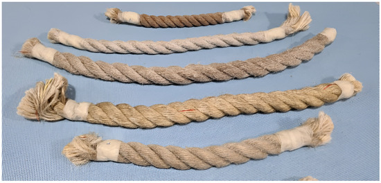
Figure 1.
Some examples of the natural fiber ropes on the ship.
However, this is a very demanding task, as regular inspection, cleaning, and proper storage are essential to maintain the integrity and longevity of ropes. Thorough inspection of the ropes is vital for detecting wear, damage, or deterioration. It is essential to examine every rope onboard, inside and out, for signs of excessive wear such as frayed or broken fibers, knots, twists, mold, or mildew. Many accidents and fatalities onboard are linked to poor rope condition and neglect [4]. To summarize, manual inspection procedures are labor intensive, time-consuming and subjective.
The monitoring and maintenance of ropes and cables are critical across a wide range of industries, including construction [5,6], offshore drilling [7], mining [8], and maritime transport [9,10].
In fields such as mountaineering, cable-driven transport, and naval operations, sensor-based approaches (e.g., tension measurements, magnetic flux leakage for steel ropes [11,12,13,14]) have emerged to complement manual methods. However, these systems often require complex equipment, offer limited automation, or are not suitable for natural fiber materials such as manila ropes.
With the advancement of artificial intelligence, particularly machine learning (ML) [15] and computer vision [16], a new generation of rope inspection systems has become possible.
In the context of image-based tasks, convolutional neural networks (CNNs) [17] have become the go-to architecture. CNNs have been used in a number of applications in research, from pattern recognition [18], speech recognition [19,20], image recognition [21,22], behavior detection [23,24], text classification [25,26], and more.
CNNs are especially powerful in analyzing visual data: they can automatically extract and learn relevant features (such as textures, shapes, or surface damage) from raw images, enabling accurate classification or detection of specific conditions. This has made them a natural fit for condition monitoring tasks where subtle visual cues indicate material fatigue, wear, or structural failure.
At its core, ML allows a computer model to recognize patterns—such as signs of wear or damage—by training on labeled examples. Recent work has demonstrated the feasibility and effectiveness of ML-based rope monitoring systems. For instance, Jalonen et al. (2023) [27] developed a lightweight CNN for real-time degradation detection in synthetic lifting ropes, achieving high classification accuracy with minimal memory requirements. Similarly, Rani et al. (2023) [28] utilized Mask R-CNN via Detectron2 to segment and identify specific rope defects such as chafing, placking, and unwinding. These models enable fine-grained localization of wear and damage.
Recent studies have demonstrated the effectiveness of deep learning models in fault detection tasks in various industrial applications. For example, Siddique et al. (2025) [29] proposed a CNN-based approach for diagnosing faults in centrifugal pumps using time-frequency image representations derived from vibration signals, achieving near-perfect classification accuracy. Although their domain differs, the use of CNNs for discriminative feature extraction and the focus on embedded applicability parallel the objectives of our work in maritime rope monitoring.
Zhou et al. (2018) [30] used a convolutional neural network (CNN)-based method to monitor the health condition of the balancing tail ropes (BTRs), detecting various BTR faults in real-time, including disproportional spacing, twisted rope, broken strands and broken rope faults.
Several recent studies have explored advanced approaches for steel wire rope defect detection. Delimayanti et al. (2024) [31] employed transfer learning techniques to detect surface defects on elevator steel wire ropes, demonstrating how pre-trained convolutional neural networks can be adapted to rope monitoring with improved accuracy and reduced training time. Their approach highlights the practical benefits of leveraging existing deep learning models to overcome limited domain-specific datasets. Wang et al. (2023) [32] introduces a CNN-Transformer model combined with transfer learning for wire rope defect diagnosis. Similarly, Bao and Hu (2024) [33] proposed a novel optical non-destructive testing method for steel ropes that integrates high-resolution imaging with machine learning algorithms, enabling rapid identification of damage without compromising the rope’s integrity. Peng et al’s. (2024) [34] method for identifying steel wire rope damage width utilizes ResNet50 on time-spectrum images derived from magnetic flux leakage data. The detection accuracy is reported as 97%. Huang et al. (2020) [35] proposed a CNN-based method for steel wire ropes surface damage detection, designing their own data acquisition apparatus, obtaining an F1 score of 0.99. Additional work by Falconer (2022) [36] explored machine learning models for rope condition monitoring under cyclic bend-over-sheave testing, incorporating computer vision, thermal data, and Remaining Useful Life (RUL) prediction—an approach that blends ML with predictive maintenance goals.
Eventually, a 2024 review published in Engineering Applications of AI [37] provides a comprehensive overview of ML-based synthetic fiber rope monitoring, including supervised and semi-supervised learning, generative data augmentation, and challenges related to labeled data scarcity.
Despite the focus on synthetic and steel ropes, there is a growing opportunity to adapt these technologies to natural fiber ropes, such as the manila ropes used aboard the historic training ship Amerigo Vespucci.
Most existing rope monitoring systems are designed for synthetic or steel ropes, which are commonly used in modern industrial, maritime, or construction contexts. These materials often allow integration with embedded sensors (e.g., tension, strain, or fiber optics) and typically degrade in more predictable patterns. In contrast, natural fiber ropes, such as those used aboard the Amerigo Vespucci, pose unique challenges: they are highly sensitive to environmental factors (e.g., moisture, UV exposure, salt), their wear tends to be visually irregular and surface-driven, and their structure precludes sensor embedding without damaging integrity. Our approach explicitly addresses these issues by using non-invasive, visual monitoring techniques tailored to the complex texture and fraying patterns of natural fibers. The image-based method allows for preservation-sensitive monitoring, making it particularly suited for use aboard historic or traditionally rigged vessels where modern instrumentation is impractical or undesirable. This article introduces a novel ML-based device designed to classify the level of degradation in manila ropes through image-based inspection.
This work is part of a multidisciplinary project resulting from the collaboration between the University of Genoa and the Italian Hydrographic Institute (Istituto Idrografico della Marina). The project aims to advance scientific research conducted aboard the Amerigo Vespucci during its world tour 2023–2025 [2,38].
In this work, we want to create a system that aims to provide efficient, non-invasive assessment directly onboard, preserving both operational safety and the authenticity of heritage maritime equipment, leveraging lightweight convolutional neural networks.
2. Materials and Methods
2.1. The Device
The choice of an embedded system, specifically a Raspberry Pi 3 (Sony UK Technology Centre, Pencoed, Wales, UK), was motivated by the operational constraints aboard the Amerigo Vespucci. These include limited physical space, the absence of reliable internet connectivity, and the need for a portable, low-power, and autonomous inspection tool that can be easily used by non-technical crew members. Unlike cloud-based or desktop solutions, embedded systems offer a self-contained platform for both data acquisition and onboard inference, making real-time monitoring feasible in maritime environments.
The Raspberry Pi 3 provides a balance between performance and energy efficiency, and its compatibility with camera modules and 3D-printed enclosures further supports field deployment in challenging conditions. The device has been specifically developed to capture high-quality images of the ropes aboard the historic training ship Amerigo Vespucci. Its primary objective is to document the physical condition of the ropes for analysis, maintenance, and archival purposes. The device is enclosed in a custom-designed 3D-printed case, which provides protection to the inside components against the demanding conditions typically found at sea. Inside the casing is a Raspberry Pi 3 Model B+ paired with the Raspberry Pi Camera Module V2 (Sony UK Technology Centre, Pencoed, Wales, UK), which uses a Sony IMX219 8-megapixel sensor with a fixed focus lens. Videos are captured at a resolution of 720 × 480 pixels and a frame rate of 25 fps (information about software and libraries used is specified in Appendix A). Additionally, the system includes internal memory storage for saving captured images locally, as well as a rechargeable battery that enables the device to operate independently of external power sources. This autonomy is essential for use onboard, especially in environments where power supply and internet connectivity may be limited or unavailable. The exterior of the device features a user-friendly interface consisting of a power button to switch the device on and off, and two separate buttons dedicated to taking photographs. Around the camera there are 2 strips of LED lights, programmed to turn on when the button to capture images is pressed. These are thought to provide the same amount of light for each picture (Figure 2).
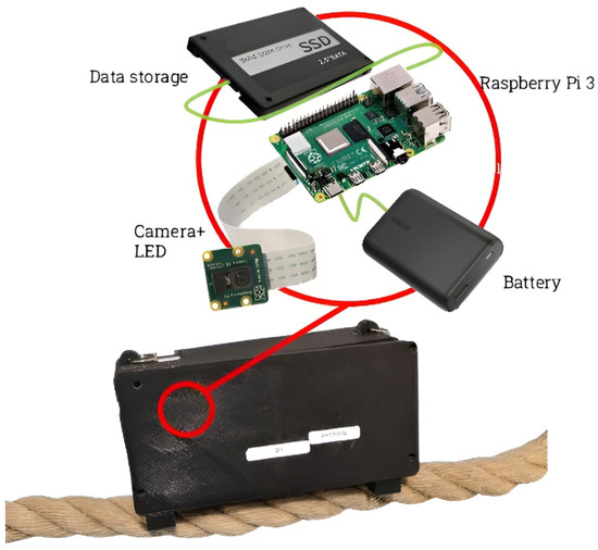
Figure 2.
The MonCord device, with its principal component.
Its compact, portable design and self-sufficiency make it well-suited for maritime environments, enabling the crew or researchers to easily carry and operate it throughout the vessel without requiring technical expertise or constant network access.
2.2. Dataset Collection and Splitting
The device described above is subsequently deployed aboard the Amerigo Vespucci. A comprehensive instruction manual is provided to the crew to guide them in its use for data collection purposes.
The crew is also provided with two 3D-printed squares, one green and one red, to use during data collection. They are instructed to display the appropriate square before recording video footage of a rope: the green square indicates that the rope is in good condition, while the red square indicates that the rope is in poor condition and needs replacement. In total, 207 recordings of ropes are collected.
Once returned to the ground, the 207 recordings are extracted. Out of those, 121 show the red square while only 16 show the green one. The remaining recordings either do not depict ropes or lack the color indicator preceding the footage, rendering them not usable for classification tasks; hence, they are discarded. An additional eight recordings labeled with the red square are excluded due to poor image quality. From the remaining set, 29 recordings depicting damaged ropes are manually selected. All 16 recordings showing ropes in good condition are retained.
From the selected recordings, a set of frames is extracted to create an initial raw dataset. The procedure involves extracting all frames from each video: among these, the ones not picturing ropes are discarded. To eliminate blurry images, the variance of the Laplacian [39] is computed for each frame. Images with a variance below a predefined threshold are classified as blurry and subsequently eliminated; otherwise, the image is kept in the dataset.
From this pool of images, 1200 frames for each class (“red” and “green”) are randomly selected to create the raw dataset. Some examples are shown in Figure 3.
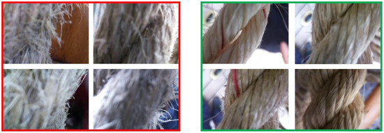
Figure 3.
Example of the images taken on the ship. Circled in red: examples of ruined ropes; in green: the good ones.
Based on input from the crew, the primary indicators distinguishing a good rope from a degraded one are as follows: The most critical factor is the presence of “fuzziness” on the rope’s surface, which results from friction between the rope and various elements of the ship. A secondary indicator is bacterial degradation, typically evidenced by visible spotting on the rope. Keeping in mind this information, the images are preprocessed in the following way to pass through a neural network (Figure 4):
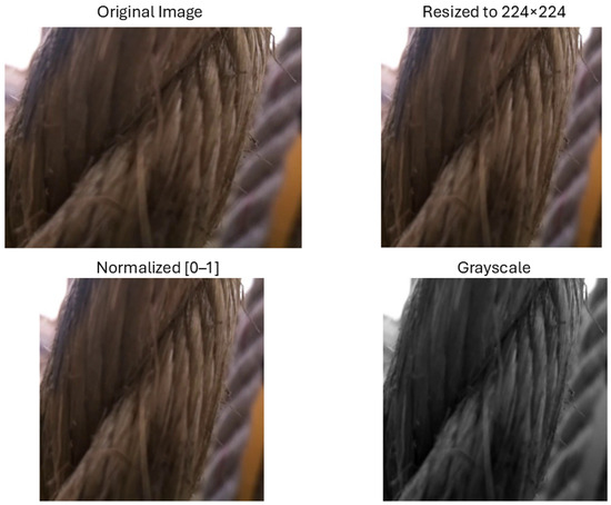
Figure 4.
Example of the preprocessing steps.
- Image Resizing. All images must be resized in the same shape. CNNs require all input images to have the same dimensions so that the network’s architecture can process them uniformly.
- Normalization. Through image normalization, the model trains more efficiently by stabilizing gradients, speeding up convergence, and reducing the risk of numerical issues. It also prevents certain pixels from dominating the learning process due to larger values and improves the model’s ability to generalize to new data.
- Grayscaling. Grayscale images can simplify the problem by reducing noise related to color variations, allowing the model to focus more on shape and structure, and reducing the computational cost of the network. On the other hand, grayscaling can lead to loss of information related to the color of the image. Both approaches (grayscaling and keeping the colors) are attempted.
The detailed image preprocessing pipeline is presented in Appendix C, while all information about software and libraries is in Appendix A.
The dataset is then divided in three parts: 70% Training Set, 15% for the Validation Set and 15% for the Test Set.
To mitigate the risk of overfitting and reduce redundancy due to high frame similarity within individual recordings, we ensured that frames extracted from the same video were never shared across the training, validation, and test sets. Data augmentation is used to artificially expand the training dataset and improve the generalization of the model. By randomly flipping images horizontally and applying small rotations, the model is exposed to varied perspectives of the same data, helping it to become more robust to variations in orientation and positioning.
More aggressive transformations, such as blur, noise, or strong brightness alterations, were intentionally avoided. This decision aligns with the controlled conditions under which the images were captured using a custom-designed device, where the goal was to ensure consistent, high-quality data acquisition. We acknowledge that more extensive augmentation may be beneficial in less controlled environments.
2.3. Proposed Models
The task of classifying rope images into two categories is a binary image classification problem. Given the texture-heavy nature of the visual cues (e.g., surface fuzziness, fraying, and spotting), the model must be capable of extracting fine-grained local features while maintaining robustness to noise, blur, and lighting variations commonly present in real-world maritime conditions.
To address these requirements, we evaluated two main strategies:
- Custom CNN Architectures.
The custom models allowed for greater flexibility in incorporating domain-specific preprocessing (e.g., grayscale input, texture emphasis) and experimenting with input sizes, kernel shapes, and activation functions.
In addition to experiments with pre-trained models, a custom convolutional neural network (CNN) was developed specifically for the binary classification of rope images. The architecture consists of convolutional blocks, composed by a Conv2D layer with ReLU activation followed by a MaxPooling2D layer for spatial downsampling. The convolutional output is then flattened and passed through a fully connected dense layer with 128 units, followed by a dropout layer with a dropout rate of 0.5 to mitigate overfitting. The final output layer consists of a single neuron with a sigmoid activation function, suitable for binary classification tasks. A diagram of the network architecture is shown in Figure 5.
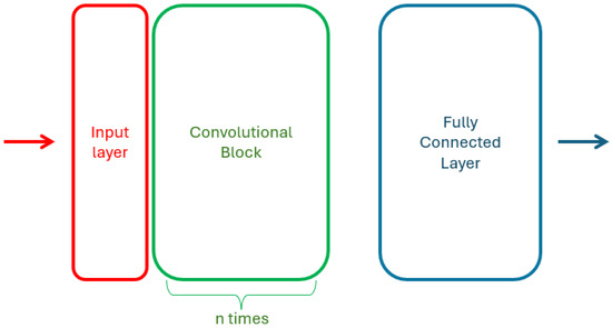
Figure 5.
Structure of a custom model CNNn architecture.
Several variations were tested to explore the impact of architectural depth and input format on classification performance. Specifically, both grayscale and color image inputs were used across experiments to assess how color information affected the model’s ability to distinguish between damaged and undamaged ropes. For each input type, the network architecture was modified by adding a varying number of additional convolutional blocks at the beginning of the model. All architecture are summarized in the Table A1 in Appendix B.
All input images were resized to 128 × 128 pixels and normalized to the [0, 1] range. The network was trained using the Adam optimizer with a learning rate of 1 × 10⁻⁴ and binary cross-entropy as the loss function. Training was performed over 30 epochs with a batch size of 32. Early stopping with a patience of 5 epochs and model checkpointing based on validation loss were used to prevent overfitting and retain the best version of the model.
While the custom models offered more interpretability and control over the architecture, they typically required longer training and more careful tuning to achieve performance comparable to transfer learning approaches.
- Transfer Learning with Pre-trained Convolutional Neural Networks (CNNs).
Transfer learning is a widely adopted approach in image classification tasks, particularly when the dataset size is limited. This approach provided strong baseline performance and significantly reduced the training time compared to training a model from scratch.
We experimented with pre-trained models such as MobileNetV2 [40] and EfficientNetB0 [41], both trained on the ImageNet dataset. These architectures were selected for their balance between performance and computational efficiency, as both networks are light weight and work well even on the Raspberry Pi.
For both networks, the same procedure is followed: the model is customized by removing its original classification head and adding a new output structure consisting of a global average pooling layer, a dropout layer (rate 0.3), and a final dense layer with a sigmoid activation function to produce binary predictions. A diagram of the network architecture is shown in Figure 6.
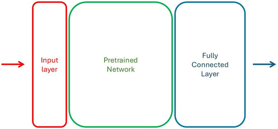
Figure 6.
Structure of the pre-trained models architecture.
Initially, all layers of the pre-trained model’s base are frozen to preserve the pre-trained weights, and only the newly added classification head is trained. The model is compiled using the Adam optimizer with a learning rate of 1 × 10⁻⁴ and binary cross-entropy as the loss function. Training is performed for 30 epochs using a batch size of 32, with data augmentation techniques, random horizontal flipping and slight rotations, applied to the training set to improve generalization.
Following this initial training phase, fine-tuning was conducted to allow the model to better adapt to the specific visual characteristics of the rope dataset. The base model was partially unfrozen, with the first 100 layers remaining frozen to retain low-level visual features. The entire model was then retrained for an additional 30 epochs with a reduced learning rate of 1 × 10⁻⁵. Throughout both training phases, early stopping with a patience of 5 epochs and model checkpointing were used to prevent overfitting and retain the best-performing model based on validation loss.
Before being input into models like MobileNetV2 and EfficientNetB0, images must be properly preprocessed to match each model’s expected format. Both models require images to be resized to 224 × 224 pixels, which is their standard input size. However, they differ in how pixel values are scaled: MobileNetV2 expects pixel values in the range [−1, 1], while EfficientNetB0 expects values in the range [0, 255] but internally scales and normalizes them using its own preprocessing. To handle these differences correctly, TensorFlow provides model-specific preprocessing functions for MobileNetV2 [42] and for EfficientNetB0 [43]. Using these ensures that the inputs are consistent with how the models were originally trained, leading to better performance and more reliable predictions.
The experiments’ codes were written in Python 3 [44] using Tensorflow 2 [45] and are publicly available.
2.4. Evaluation Metrics
In order to compare different models and classifiers performances on both training and test sets, some parameters must be identified that will allow comparison.
Models were evaluated based on classification accuracy on a held-out test set; precision, recall, and F1-score to assess class-specific performance, especially important due to potential class imbalance [46].
Accuracy is the simplest metric to use and implement, it is defined as the percentage of correct predictions over the total number of predictions. Accuracy provides a general indication of how effectively the network classifies images. Precision is the ratio of true positives over the total number of positives predicted while Recall is the ratio of true positives over all the positives predicted by the model. The F1 score combines precision and recall to provide an objective measure of a classification method’s overall generalization performance. The Confusion Matrix is not a metric, but provides a visualization of the performance of an algorithm in a table layout. The name stems from the fact that it makes it easy to see how much the system is confusing two classes. In the case of a perfect classifier the matrix would be diagonal.
where TP, TN, FP, and FN are true positives, true negatives, false positives, and false negatives, respectively (positive/negative denotes a damaged/normal rope).
Another useful tool to evaluate the performance of the models is t-distributed Stochastic Neighbor Embedding (t-SNE) [47], a nonlinear technique designed specifically to visualize high-dimensional data in 2D or 3D. t-SNE is commonly used to inspect learned representations in deep learning, visualizing how well a model separates different classes. If each class forms a separate cluster in t-SNE, the model likely learned meaningful features.
3. Results
The performance of the proposed models was evaluated on the held-out test set using accuracy, precision, recall, and F1-score as defined earlier. Table 1 summarizes the quantitative results for each configuration.

Table 1.
Performance of different models on the test set.
The performance of both transfer learning models and the custom CNNs is evaluated on the test dataset. Evaluation metrics include accuracy, precision, recall, and F1-score, providing a comprehensive view of each model’s ability to distinguish between intact and damaged ropes.
The results from the training of the custom CNNs clearly show better performance when the images are in color than in grayscale: for each variation of the convolutional blocks, the color images version performed better in each metric. This suggests that while grayscale preprocessing reduces computational complexity and noise, it also discards useful visual cues, particularly those related to color-based degradation patterns. As a result, models trained on grayscale images tended to have a higher false negative rate. For this reason, the pre-trained models are trained only on color images.
The pre-trained models achieved the highest overall accuracy and F1-score, benefiting from pre-trained features and fine-tuning on rope images. The custom CNNs, while having fewer parameters and a simpler architecture, performed competitively and demonstrated good generalization.
Training and validation loss curves indicate that all models benefited from early stopping and dropout regularization.
Transfer learning models reached convergence more rapidly and exhibited smaller gaps between training and validation loss, while custom CNNs showed greater sensitivity to overfitting. Fine-tuning pre-trained models improved performance marginally but consistently across all metrics. Figure 7, Figure 8 and Figure 9 show the training and validation accuracy and loss curves for each transfer model and the best performing custom CNN, CNN5. The based model exhibited rapid convergence during the initial training phase, followed by further improvements during fine-tuning. The custom CNN converged more slowly and was more sensitive to overfitting, but still achieved respectable performance with early stopping and data augmentation.
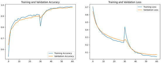
Figure 7.
EfficientNetB0 training/validation accuracy/loss.
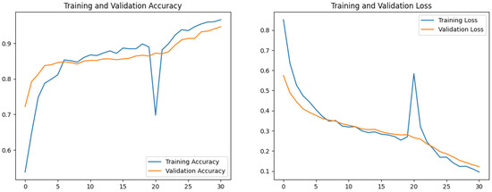
Figure 8.
MobileNetV2 training/validation accuracy/loss.
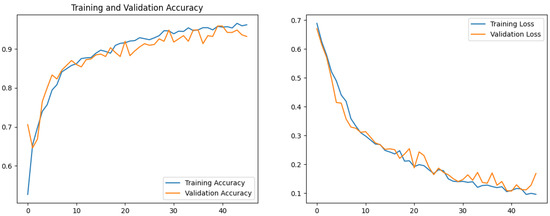
Figure 9.
Custom CNN (CNN5) training/validation accuracy/loss.
To gain more insight into the classification behavior, confusion matrices were generated for the models (Figure 10, Figure 11 and Figure 12). We labeled True Positive (TP): Correctly identified damaged ropes, True Negative (TN): Correctly identified intact ropes, False Positive (FP): Intact rope misclassified as damaged and False Negative (FN): Damaged rope misclassified as intact. The EfficientNetB0 and MobileNetv2 models showed fewer false positives and false negatives, while the custom CNN had a slightly higher false negative rate, misclassifying some damaged ropes as intact.
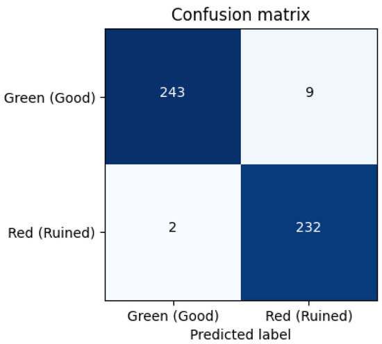
Figure 10.
EfficientNetB0 Confusion Matrix.
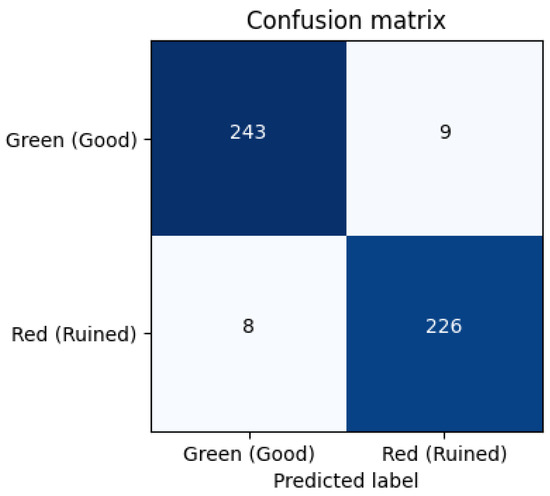
Figure 11.
MobileNetv2 Confusion Matrix.

Figure 12.
CNN5 Confusion Matrix.
Since the model will be implemented on the mobile device, it is essential to consider not only its performance during training but also practical deployment factors. Model size, inference time, and overall resource efficiency play a crucial role in determining suitability for mobile environments. The following table (Table 2) presents a comparison of the top three models with respect to these deployment considerations. Inference time is averaged over 500 inferences and the error is obtained as the standard deviation of these times.
Table 2.
Performance of different models.
Moreover, the t-sne results in Figure 13 show good class separation for all three models, although t-SNE shows few rope images labeled as normal within the damaged rope support and vice versa.
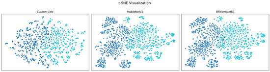
Figure 13.
t-sne visualization for the second to last layers of the three models (perplexity = 30, learning rate = 200). The two colors indicate the separation into the two classes.
We investigate some examples of misclassificated images to understand the reason behind the error.
One limitation of this study lies in the binary labeling of rope conditions as either “intact” or “damaged.” In practice, some samples could exhibit intermediate wear, such as light fraying or discoloration, that could not clearly fit either category, as is seen in some misclassified images in Figure 14 and Figure 15. These borderline cases introduce subjectivity during labeling and can affect the model’s ability to learn distinct class boundaries, potentially increasing misclassification rates. Introducing a third, intermediate class (e.g., “yellow” for partially worn ropes) could help capture the continuum of rope degradation more accurately and enable more nuanced, actionable predictions in real-world applications.
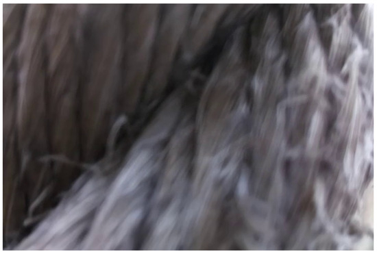
Figure 14.
Example of a “green” rope classified as “red”.
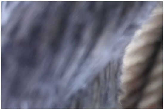
Figure 15.
Example of a “red” rope classified as “green”.
4. Discussion and Conclusions
In this work, we presented a complete pipeline for the development of an image-based system to assess the condition of maritime ropes, from data collection and labeling to model training, evaluation, and deployment considerations.
Currently, rope inspection duties aboard the Amerigo Vespucci are the responsibility of the boatswain, requiring expert manual evaluation. The proposed device enables other crew members to assist in the inspection process by capturing labeled images, which are then processed by the onboard model. This approach reduces inspection time, distributes workload, and allows for early identification of rope wear, even by non-specialists.
A custom data acquisition strategy was implemented aboard the Amerigo Vespucci, involving manual labeling using color-coded indicators and the extraction of frames from recorded footage. The resulting dataset was carefully curated and preprocessed to ensure the consistency and relevance of the input data.
To address the classification task, we developed and compared two main approaches: custom convolutional neural networks (CNNs) designed from scratch, and transfer learning models based on MobileNetV2 and EfficientNetB0. Through extensive experimentation, we demonstrated that while grayscale preprocessing can reduce computational complexity, retaining color information leads to more accurate predictions—especially in detecting subtle indicators of rope degradation such as discoloration and spotting. Both custom and pre-trained models were evaluated using accuracy, precision, recall, and F1-score, supported by confusion matrices and training validation curves.
The results indicate that pre-trained models, particularly EfficientNetB0, significantly outperform custom CNNs in terms of both classification accuracy and generalization capability. Furthermore, these models benefit from faster convergence, improved stability during training, and compatibility with deployment on low-power devices. Nonetheless, the custom CNNs offered reasonable performance and greater architectural flexibility, making them suitable for contexts where model interpretability or training control is prioritized.
In addition to model accuracy, we discussed practical deployment aspects such as inference speed and resource requirements, which are critical for onboard implementation. Given its high performance and efficiency, EfficientNetB0 emerged as the most suitable model for real-world deployment in the maritime setting.
Compared to existing works in the literature, our method achieves competitive or superior performance. For instance, Jalonen et al. [27] reported an F1-score of 96.5% using a lightweight CNN on synthetic fiber ropes, while our approach achieves an F1-score of 97.68% on natural fiber ropes using EfficientNetB0. Rani et al’s. [28] segmentation-based approach using Mask R-CNN provides fine-grained detection but is computationally intensive and unsuitable for embedded deployment. In contrast, our model runs in real-time on a Raspberry Pi 3, making it more practical for maritime field use. Additionally, unlike studies focused on synthetic or steel ropes, our work addresses the unique challenges of monitoring manila ropes in maritime conditions, highlighting its broader applicability to natural fiber environments. A comparison of related studies is provided in Table 3.
Table 3.
Comparison of related works on rope/wire-rope condition monitoring.
Future work will focus on several directions aimed at extending and improving the proposed framework:
- Dataset expansion: Increase the variety and number of labeled samples to improve model generalization and capture a broader range of environmental and operational conditions.
- Temporal analysis: Explore temporal information embedded in video sequences to leverage motion cues and progressive wear patterns for more robust condition assessment.
- Embedded optimization: Further optimize real-time inference on low-power embedded hardware to enhance processing efficiency and stability during onboard operation.
- Advanced model architectures: Investigate compact transformer-based models (e.g., MobileViT, TinyViT) to determine whether attention mechanisms can enhance performance in visually complex scenarios without compromising real-time capabilities.
- Generalization improvement: Employ advanced data augmentation techniques to simulate environmental variability and generate synthetic images representing rare or hard-to-capture damage conditions.
- Multi-class classification: Extend the system from binary to multi-class labeling for more detailed rope condition assessment and more granular maintenance planning.
- Address labeling and class balance challenges: Address the difficulties introduced by multi-class expansion, including defining consistent criteria for each damage category, mitigating class imbalance, and managing subtle visual differences between classes through expert-guided labeling and improved feature extraction strategies.
Beyond the specific case of the Amerigo Vespucci, this work presents a generalizable, non-invasive framework for visual monitoring of load-bearing elements in maritime settings. While most marine inspection systems focus on structural or mechanical components using embedded sensors, natural fiber elements remain largely overlooked. The novelty of this study lies in adapting deep learning for edge-based, real-time visual assessment aboard ships—bridging a gap between modern AI techniques and the practical constraints of onboard operations. Moreover, the proposed approach is applicable to other domains where low-cost, embedded visual inspection of safety-critical components is needed, such as construction, mining, or outdoor infrastructure maintenance.
The main contributions of this study can be summarized as:
- Enabling practical rope inspections by non-specialized personnel, reducing workload and supporting early detection of wear.
- Achieving high classification accuracy and stability through transfer learning, suitable for embedded, real-time deployment.
- Providing a generalizable and scalable framework applicable to other maritime or industrial settings, including construction, mining, and outdoor infrastructure maintenance.
Ultimately, the proposed framework demonstrates the feasibility and potential of AI-assisted rope condition monitoring as a practical tool for improving safety and maintenance protocols in maritime operations.
Author Contributions
Conceptualization, M.F.; Methodology, M.F.; Software, L.R. and F.G.; Validation, M.A. and F.G.; Investigation, L.R.; Resources, M.A.; Data curation, M.A. and F.G.; Writing—original draft, L.R.; Writing—review & editing, M.F.; Supervision, M.F.; Project administration, M.A. All authors have read and agreed to the published version of the manuscript.
Funding
This research received no external funding.
Data Availability Statement
The raw data supporting the conclusions of this article will be made available by the authors on request.
Acknowledgments
The authors would like to express their sincere gratitude to the crew of the Italian training ship Amerigo Vespucci for their invaluable assistance in recording the onboard video footage used in this study. Their support and collaboration made the data collection process possible and greatly enriched the practical relevance of this work.
Conflicts of Interest
The authors declare no conflicts of interest.
Appendix A. Software and Libraries
All software development and experimentation were conducted using Python 3.12.10. The system was deployed and tested on a Raspberry Pi 3 Model B running Raspberry Pi OS (Debian-based), version 11 (Bullseye). The following libraries and frameworks were used throughout the data collection, preprocessing, model training, and evaluation pipeline:
- TensorFlow 2.19.0: Used for implementing, training, and evaluating convolutional neural networks (CNNs), including both custom architectures and pre-trained models such as MobileNetV2 and EfficientNetB0. TensorFlow was selected due to its compatibility with embedded systems through TensorFlow Lite, allowing for optimized deployment on resource-constrained hardware like the Raspberry Pi.
- OpenCV 4.12.0: Utilized for image acquisition, preprocessing, and analysis. Specifically, OpenCV was employed for applying the Laplacian variance method to assess image sharpness and filter out blurred frames. It was also used to standardize image dimensions and color spaces.
- scikit-learn 1.6.1: Used to compute evaluation metrics including accuracy, precision, recall, and F1-score. Its well-documented API and integration with NumPy made it a natural choice for model performance evaluation.
- NumPy 2.1.3: Served as the core numerical computing library for handling arrays and performing efficient matrix operations throughout the dataset preparation and model training stages.
- Matplotlib 3.10.3: Employed for visualizing training history, including accuracy and loss curves across epochs.
The choice of these specific libraries was based on their open-source availability, community support, compatibility with ARM-based systems, and ease of integration into the development pipeline.
Appendix B. Custom CNN Architectures
In the following table, the architectures of all the custom CNNs used during this study are laid out. N Block indicates how many times the convolutional block is repeated before the fully connected one.
Table A1.
Architectures of all custom CNNs used in this study. N Block indicates how many times the convolutional block is repeated before the fully connected one.
Table A1.
Architectures of all custom CNNs used in this study. N Block indicates how many times the convolutional block is repeated before the fully connected one.
| Variant N | Input Image Size | Convolutional Block | N Block | Fully Connected |
|---|---|---|---|---|
| CNN1G | 128 × 128 × 1 | 64C[3 × 3]-MP[2 × 2] | 1 | Flatten-FC[128]-D[0.5]-FC[1] |
| CNN2G | 128 × 128 × 1 | 64C[3 × 3]-MP[2 × 2] | 2 | Flatten-FC[128]-D[0.5]-FC[1] |
| CNN2 | 128 × 128 × 3 | 64C[3 × 3]-MP[2 × 2] | 2 | Flatten-FC[128]-D[0.5]-FC[1] |
| CNN3G | 128 × 128 × 1 | 64C[3 × 3]-MP[2 × 2] | 3 | Flatten-FC[128]-D[0.5]-FC[1] |
| CNN3 | 128 × 128 × 3 | 64C[3 × 3]-MP[2 × 2] | 3 | Flatten-FC[128]-D[0.5]-FC[1] |
| CNN4G | 128 × 128 × 1 | 64C[3 × 3]-MP[2 × 2] | 4 | Flatten-FC[128]-D[0.5]-FC[1] |
| CNN4 | 128 × 128 × 3 | 64C[3 × 3]-MP[2 × 2] | 4 | Flatten-FC[128]-D[0.5]-FC[1] |
| CNN5G | 128 × 128 × 1 | 64C[3 × 3]-MP[2 × 2] | 5 | Flatten-FC[128]-D[0.5]-FC[1] |
| CNN5 | 128 × 128 × 3 | 64C[3 × 3]-MP[2 × 2] | 5 | Flatten-FC[128]-D[0.5]-FC[1] |
Appendix C. Image Data Processing Pipeline
This appendix provides detailed information about the data preprocessing steps used in the creation of the training dataset, in order to ensure reproducibility and transparency.
- Labeling Strategy: Ropes were physically labeled onboard the vessel using colored tape markers placed by crew members as Green (rope in good condition) and Red (rope in poor condition). Video labels were assigned based on visible markers and verified manually. Ambiguous or unlabeled frames were excluded from the final dataset to ensure label reliability.
- Frame Extraction: Video recordings (207 total, MP4 format, 720 × 480, 25 fps) were processed using OpenCV. Frames were extracted at the original frame rate of the video. This approach was chosen to retain the full temporal resolution of the visual data and to maximize the number of high-quality rope images available for filtering and model training.
- Blur Detection and Filtering: To remove visually degraded samples, each frame was analyzed for sharpness using the Laplacian variance method. Frames with a variance score below 100 were discarded. This threshold was determined empirically to balance clarity and dataset size.
- Image Preprocessing: Remaining images were resized to 224 × 224 pixels using bilinear interpolation to standardize input dimensions for CNN models. Two variants of each image were saved: RGB format (3 channels) for color experiments and Grayscale (single channel) using OpenCV’s color to gray conversion [48]. All pixel values were normalized to the [0, 1] range.
- The dataset was curated to ensure class balance and prevent information leakage: A 70/15/15 stratified split was applied to create training, validation, and test sets. Care was taken to ensure that no frames from the same video appeared in more than one split.
- All preprocessing was performed using: Python 3.12.10, OpenCV 4.12.0, NumPy 2.1.3 and PIL (Pillow).
References
- Amerigo Vespucci. Available online: https://www.marina.difesa.it/noi-siamo-la-marina/pilastro-operativo/mezzi/forze-navali/Pagine/Vespucci.aspx (accessed on 1 July 2025).
- Amerigo Vespucci. The Ship. Available online: https://tourvespucci.it/en/the-ship/ (accessed on 1 July 2025).
- Smith, H.G. The Arts of the Sailor: Knotting, Splicing and Ropework; Dover Publications: Mineola, NY, USA, 1990. [Google Scholar]
- MAIB Safety Digests 20–24. Available online: https://www.gov.uk/government/publications/maib-safety-digests-20-24 (accessed on 1 July 2025).
- Chen, W.F.; Duan, L. Construction and Maintenance; CRC Press: Boca Raton, FL, USA, 2014. [Google Scholar]
- Kurz, J.H.; Laguerre, L.; Niese, F.; Gaillet, L.; Szielasko, K.; Tschuncky, R.; Treyssede, F. NDT for need based maintenance of bridge cables, ropes and pre-stressed elements. J. Civ. Struct. Health Monit. 2013, 3, 285–295. [Google Scholar] [CrossRef]
- Schlanbusch, R.; Oland, E.; Bechhoefer, E.R. Condition monitoring technologies for steel wire ropes—A review. Int. J. Progn. Health Manag. 2017, 8, 2527. [Google Scholar] [CrossRef]
- Ilsley, L.C.; Mosier, M. Inspection and Maintenance of Mine Hoisting Ropes; Department of the Interior, Bureau of Mines: Washington, DC, USA, 1939; Volume 602.
- Ma, K.T.; Shu, H.; Smedley, P.; L’Hostis, D.; Duggal, A. A historical review on integrity issues of permanent mooring systems. In Proceedings of the Offshore Technology Conference, OTC, Houston, TX, USA, 6–9 May 2013. [Google Scholar]
- Jiang, X. Structural integrity assessment of maritime transport equipment. In Proceedings of the International Conference on Offshore Mechanics and Arctic Engineering, Madrid, Spain, 17–22 June 2018; American Society of Mechanical Engineers: New York, NY, USA, 2018; Volume 51333. [Google Scholar]
- Galluzzi, R.; Feraco, S.; Zenerino, E.C.; Tonoli, A.; Bonfitto, A.; Hegde, S. Fatigue monitoring of climbing ropes. Proc. Inst. Mech. Eng. Part P J. Sport. Eng. Technol. 2020, 234, 328–336. [Google Scholar] [CrossRef]
- Lei, G.; Xu, G.; Zhang, X.; Zhang, Y.; Song, Z.; Xu, W. Study on dynamic monitoring of wire rope tension based on the particle damping sensor. Sensors 2019, 19, 388. [Google Scholar] [CrossRef] [PubMed]
- Witoś, M.; Zieja, M.; Żokowski, M.; Kwaśniewski, J.; Iwaniec, M. NDE of mining ropes and conveyors using magnetic methods. In Proceedings of the International Symposium on Structural Health Monitoring and Nondestructive Testing, Saarbruecken, Germany, 4–5 October 2018. [Google Scholar]
- Mazurek, P. A comprehensive review of steel wire rope degradation mechanisms and recent damage detection methods. Sustainability 2023, 15, 5441. [Google Scholar] [CrossRef]
- Alpaydin, E. Machine Learning; MIT Press: Cambridge, MA, USA, 2021. [Google Scholar]
- Ballard, D.H.; Brown, C.M. Computer Vision; Prentice Hall: Englewood, NJ, USA, 1982. [Google Scholar]
- O’shea, K.; Nash, R. An introduction to convolutional neural networks. arXiv 2015, arXiv:1511.08458. [Google Scholar] [CrossRef]
- Xie, F.; Xie, M.; Wang, C.; Li, D.; Zhang, X. PDCG-Enhanced CNN for Pattern Recognition in Time Series Data. Biomimetics 2025, 10, 263. [Google Scholar] [CrossRef]
- Huang, Z.; Dong, M.; Mao, Q.; Zhan, Y. Speech emotion recognition using CNN. In Proceedings of the 22nd ACM International Conference on Multimedia, Orlando, FL, USA, 3–7 November 2014. [Google Scholar]
- Palaz, D.; Magimai-Doss, M.; Collobert, R. Analysis of CNN-based speech recognition system using raw speech as input. In Proceedings of the Interspeech 2015, Dresden, Germany, 6–10 September 2015. [Google Scholar]
- Pak, M.; Kim, S. A review of deep learning in image recognition. In Proceedings of the 2017 4th International Conference on Computer Applications and Information Processing Technology (CAIPT), Kuta Bali, Indonesia, 8–10 August 2017. [Google Scholar]
- Chen, L.; Li, S.; Bai, Q.; Yang, J.; Jiang, S.; Miao, Y. Review of image classification algorithms based on convolutional neural networks. Remote Sens. 2021, 13, 4712. [Google Scholar] [CrossRef]
- Wastupranata, L.M.; Kong, S.G.; Wang, L. Deep learning for abnormal human behavior detection in surveillance videos—A survey. Electronics 2024, 13, 2579. [Google Scholar] [CrossRef]
- Siddique, M.F.; Zaman, W.; Umar, M.; Kim, J.-Y.; Kim, J.-M. A Hybrid Deep Learning Framework for Fault Diagnosis in Milling Machines. Sensors 2025, 25, 5866. [Google Scholar] [CrossRef]
- Palanivinayagam, A.; El-Bayeh, C.Z.; Damaševičius, R. Twenty years of machine-learning-based text classification: A systematic review. Algorithms 2023, 16, 236. [Google Scholar] [CrossRef]
- Gasparetto, A.; Marcuzzo, M.; Zangari, A.; Albarelli, A. A survey on text classification algorithms: From text to predictions. Information 2022, 13, 83. [Google Scholar] [CrossRef]
- Jalonen, T.; Al-Sa’d, M.; Mellanen, R.; Kiranyaz, S.; Gabbouj, M. Real-time damage detection in fiber lifting ropes using convolutional neural networks. arXiv 2023, arXiv:2302.11947. [Google Scholar] [CrossRef]
- Rani, A.; Ortiz-Arroyo, D.; Durdevic, P. Defect detection in synthetic fibre ropes using detectron2 framework. Appl. Ocean. Res. 2024, 150, 104109. [Google Scholar] [CrossRef]
- Siddique, M.F.; Ullah, S.; Kim, J.M. A Deep Learning Approach for Fault Diagnosis in Centrifugal Pumps through Wavelet Coherent Analysis and S-Transform Scalograms with CNN-KAN. Comput. Mater. Contin. 2025, 84, 3577–3603. [Google Scholar] [CrossRef]
- Zhou, P.; Zhou, G.; Zhu, Z.; Tang, C.; He, Z.; Li, W.; Jiang, F. Health monitoring for balancing tail ropes of a hoisting system using a convolutional neural network. Appl. Sci. 2018, 8, 1346. [Google Scholar] [CrossRef]
- Wardhani, N.; Heriyanto, R.A.W.; Nainggolan, S.P. Detection of Steel Wire Rope Surface Defects on Elevators: A Transfer Learning Approach. Available online: https://www.icmlc.com/technicalProgram/2025/FP/1166.pdf (accessed on 27 October 2025).
- Wang, M.; Li, J.; Xue, Y. A New Defect Diagnosis Method for Wire Rope Based on CNN-Transformer and Transfer Learning. Appl. Sci. 2023, 13, 7069. [Google Scholar] [CrossRef]
- Bao, Y.; Hu, B. A New Method For Optical Steel Rope Non-Destructive Damage Detection. In Proceedings of the 2024 2nd International Conference on Intelligent Perception and Computer Vision (CIPCV), Xiamen, China, 17–19 May 2024; pp. 87–95. [Google Scholar] [CrossRef]
- Peng, Y.; Liu, J.; He, J.; Qiu, Y.; Liu, X.; Chen, L.; Yang, F.; Chen, B.; Tang, B.; Wang, Y. Steel Wire Rope Damage Width Identification Method Based on Residual Networks and Multi-Channel Feature Fusion. Machines 2024, 12, 744. [Google Scholar] [CrossRef]
- Huang, X.; Liu, Z.; Zhang, X.; Kang, J.; Zhang, M.; Guo, Y. Surface damage detection for steel wire ropes using deep learning and computer vision techniques. Measurement 2020, 161, 107843. [Google Scholar] [CrossRef]
- Falconer, S.; Krause, P.; Bäck, T.; Nordgård-Hansen, E.; Grasmo, G. Condition classification of fibre ropes during cyclic bend over sheave testing using machine learning. Int. J. Progn. Health Manag. 2022, 13, 3105. [Google Scholar] [CrossRef]
- Rani, A.; Ortiz-Arroyo, D.; Durdevic, P. A survey of vision-based condition monitoring methods using deep learning: A synthetic fiber rope perspective. Eng. Appl. Artif. Intell. 2024, 136, 108921. [Google Scholar] [CrossRef]
- UniGe e Istituto Idrografico Fanno Ricerca a Bordo Del Vespucci. Available online: https://life.unige.it/progetto-vespucci-sett2023 (accessed on 1 July 2025).
- Pech-Pacheco, J.L.; Cristobal, G.; Chamorro-Martinez, J.; Fernandez-Valdivia, J. Diatom autofocusing in brightfield microscopy: A comparative study. In Proceedings of the 15th International Conference on Pattern Recognition, ICPR-2000, Barcelona, Spain, 3–7 September 2000; Volume 3, pp. 314–317. [Google Scholar] [CrossRef]
- Sandler, M.; Howard, A.; Zhu, M.; Zhmoginov, A.; Chen, L.C. Mobilenetv2: Inverted residuals and linear bottlenecks. In Proceedings of the IEEE Conference on Computer Vision and Pattern Recognition, Salt Lake City, UT, USA, 18–22 June 2018. [Google Scholar]
- Tan, M.; Le, Q. Efficientnet: Rethinking model scaling for convolutional neural networks. In Proceedings of the International Conference on Machine Learning, PMLR, Long Beach, CA, USA, 9–15 June 2019. [Google Scholar]
- MobileNetV2 Preprocessing Layer. Available online: https://www.tensorflow.org/api_docs/python/tf/keras/applications/mobilenet_v2/preprocess_input (accessed on 27 October 2025).
- EfficientNetB0 Preprocessing Layer. Available online: https://www.tensorflow.org/api_docs/python/tf/keras/applications/efficientnet/preprocess_input (accessed on 27 October 2025).
- Python. Python Releases for Windows 24. 2021. Available online: https://www.python.org/downloads/windows/ (accessed on 27 October 2025).
- Zenodo. TensorFlow, version 2.19.0; CERN: Geneva, Switzerland, 2022.
- Handelman, G.S.; Kok, H.K.; Chandra, R.V.; Razavi, A.H.; Huang, S.; Brooks, M.; Lee, M.J.; Asadi, H. Peering into the black box of artificial intelligence: Evaluation metrics of machine learning methods. Am. J. Roentgenol. 2019, 212, 38–43. [Google Scholar] [CrossRef]
- Maaten, L.V.D.; Hinton, G. Visualizing data using t-SNE. J. Mach. Learn. Res. 2008, 9, 2579–2605. [Google Scholar]
- Open Cv cv2.COLOR_BGR2GRAY. Available online: https://docs.opencv.org/3.4/d8/d01/group__imgproc__color__conversions.html (accessed on 27 October 2025).
Disclaimer/Publisher’s Note: The statements, opinions and data contained in all publications are solely those of the individual author(s) and contributor(s) and not of MDPI and/or the editor(s). MDPI and/or the editor(s) disclaim responsibility for any injury to people or property resulting from any ideas, methods, instructions or products referred to in the content. |
© 2025 by the authors. Licensee MDPI, Basel, Switzerland. This article is an open access article distributed under the terms and conditions of the Creative Commons Attribution (CC BY) license (https://creativecommons.org/licenses/by/4.0/).