Abstract
Turbidity currents are important carriers for transporting terrestrial sediment into the deep sea, facilitating the transfer of matter and energy between land and the deep sea. Previous studies have suggested that turbidity currents can exhibit high velocities during their movement in submarine canyons. However, the maximum vertical descent velocity of high-concentration turbid water simulating turbidity currents does not exceed 1 m/s, which does not support the understanding that turbidity currents can reach speeds of over twenty meters per second in submarine canyons. During their movement, turbidity currents can compress and push the water ahead, generating propagating waves. These waves, known as excitation waves, exert a force on the seafloor, resuspending bottom sediments and potentially leading to the generation of secondary turbidity currents downstream. Therefore, the propagation distance of excitation waves is not the same as the initial journey of the turbidity currents, and the velocity of excitation waves within this journey has been mistakenly regarded as the velocity of the turbidity currents. Research on the propagation velocity of excitation waves is of great significance for understanding the sediment supply patterns of turbidity currents and the transport patterns of deep-sea sediments. In this study, numerical simulations were conducted to investigate the velocity of excitation waves induced by turbidity currents and to explore the factors that can affect their propagation velocity and amplitude. The relationship between the velocity and amplitude of excitation waves and different influencing factors was determined. The results indicate that the propagation velocity of excitation waves induced by turbidity currents is primarily determined by the water depth, and an expression (v2 = 0.63gh) for the propagation velocity of excitation waves is provided.
1. Introduction
Submarine turbidity currents, often referred to as underwater rivers, are important carriers that transport terrestrial sediments to the deep sea [1,2,3,4,5,6,7]. These turbidity currents, carrying a large amount of silt and sand, not only have strong erosive capabilities on the seabed [8,9,10], but also pose a threat to underwater communication cables, resulting in significant economic losses [11,12,13]. For example, the 2006 Pingdong earthquake in Taiwan caused the rupture of 11 submarine cables within the Kaoping Canyon, resulting in a slowdown in network speed in Southeast Asia for 49 days and requiring the deployment of 11 cable ships for repairs [13,14,15]. Investigating the velocity and patterns of turbidity currents in submarine canyons is of great significance for the protection of infrastructure such as pipelines and cables in these canyons.
One of the main methods for quantitatively studying the velocity of turbidity currents in submarine canyons is to infer their speed through cable ruptures. The first confirmed occurrence of cable rupture caused by a turbidity current was in 1929, when the Grand Banks earthquake triggered the continuous rupture of 12 submarine cables. Inferred maximum turbidity current velocities reached 28 m/s [16,17,18]. Subsequently, multiple cable rupture incidents caused by turbidity currents have occurred worldwide. Table 1 summarizes the inferred maximum turbidity current velocities from these cable rupture incidents.

Table 1.
Cable breakage events caused by turbidity currents worldwide.
Previous studies have shown that the maximum vertical velocity of high-concentration turbidity currents in water does not exceed 1 m/s, and the maximum downward velocity of spherical particles in water does not exceed 10 m/s [31]. The maximum velocity of professional athlete Usain Bolt in the 100 m sprint on land is 9.58 m/s, while dolphins in the ocean can reach speeds of up to 20 m/s. Deep-sea turbidity currents, characterized by a small density difference compared to water, are primarily driven by the gravitational component along the direction of flow. However, factors such as bed friction also need to be considered. The driving force behind turbidity currents is primarily the density difference between the turbulent flow and the surrounding water, as well as the gravitational downslope component. Previous studies have detected a maximum sediment concentration of 12% in the basal layer of turbidity currents [32]. However, even high concentrations of suspended sediment, such as 1720 g/L, in seawater with a density of 1020 g/L, do not exceed a maximum vertical velocity of 1 m/s [33]. Similarly, spherical particles also have a maximum settling velocity in water of less than 10 m/s [33]. Turbidity currents, being density-driven flows, have relatively low density differences compared to water, and the gentle slope of submarine canyons also contributes to a smaller gravitational downslope force. Additionally, the influence of bed friction and other factors related to sediment deposition needs to be considered. It is incredible to think that turbidity currents can achieve flow velocities as high as 28 m/s [16,18,28,34,35].
When submarine landslides occur on continental slopes, the sliding mass entering the bottom of submarine canyons can cause the destruction of soft sediment beds. The mixing of sliding or flowing sediment with water forms turbidity currents. Turbidity currents exert pressure and propel the water ahead, forming an excitation wave. This aligns with Paull’s hypothesis that in the course of turbidity currents, a high-pressure zone is formed ahead, capable of causing an increase in pore water pressure in the sediment ahead [36]. Similar to surging waves, the excitation waves generated can propagate downstream along the submarine canyon, with a propagation velocity much greater than the velocity of turbidity currents [31]. The rapid propagation of excitation waves can exert a force on the seafloor of the submarine canyon, causing the resuspension of sediment in front of the head of the turbidity currents, which may lead to the formation of secondary turbidity currents at some downstream locations. The distance between the secondary and initial turbidity currents is actually the propagation distance of the excitation waves, rather than the journey of the initial turbidity currents. Therefore, the speed of the excitation waves within this distance is mistakenly considered as the velocity of the turbidity currents (see Figure 1). This may explain why the velocity of the turbidity currents as deduced from cable breakages is so high.
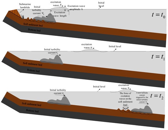
Figure 1.
Diagram of excitation wave propagation due to turbidity current (v1 is the velocity of turbidity current. This refers to the ratio of distance to time experienced by a turbidity current mass moving underwater. v2 is the velocity of secondary turbidity current: the rapidly propagating excitation wave applies a force on the submarine canyon floor, leading to the destruction of the soft sediment floor and the secondary turbidity current. v is the propagation velocity of the excitation wave; this refers to the propagation velocity of the turbidity current excitation wave. This speed is not the velocity of the motion of the water mass. At time t0, the initial turbidity current moves underwater, pushing the stationary water in front to generate an excitation wave. At time t1, the excitation wave is propagating. At time t2, the rapidly propagating excitation wave exerts pressure on the soft bottom bed, resulting in the destruction of the bottom bed and secondary turbidity current).
Turbidity currents are mass movements composed of sediment particles, with a high concentration of the dense basal layer near the seabed. Depending on their density and granulometric composition, turbidity currents can move along submarine canyons through mechanisms such as diffusion, collapse, and flow [37], which differ from the downward movement as a single entity of landslide bodies after slope failure (this distinguishes them from surges). Additionally, during the long-distance movement of turbidity currents in canyons, the completion of subsequent water replenishment may generate multiple excitation waves. Furthermore, secondary excitation waves may also occur during the movement of secondary turbidity currents triggered by the initial turbidity current, which differs significantly from the surges caused by submarine landslides. Furthermore, previous studies [38,39,40,41] on sediment supply during turbidity current movements have mostly focused on the scouring action on the seabed, whereas the resuspension of sedimentary deposits in front of the initial turbidity current caused by excitation waves may serve as an effective mode of sediment supply during the long-distance transport of turbidity currents.
In 2023, Ren et al. proposed that the cause of the long-distance high-speed motion of turbidity currents is due to the excitation waves caused by the primary turbidity currents. However, only preliminary research has been conducted on the comparison of excitation wave velocity and solitary wave velocity, and there has been no specific discussion on the reasons for the excitation wave velocity being much greater than that of the turbidity current. In an experiment conducted using an indoor flume, it was observed that the wavelength of the excitation waves was much larger than the water depth, similar to shallow water waves [33]. The amplitude of excitation waves in proportion to their wavelength was small, consistent with the theory of small-amplitude waves. Similar to the velocity model of shallow water waves, it is expected that the propagation speed of excitation waves is also influenced by the water depth. However, since excitation waves are triggered by sediment-laden turbidity currents, the velocity model may differ from that of surface waves induced by gravitational flows.
The purpose of this study is to simulate and investigate the effects of different factors on the propagation velocity and amplitude of excitation waves through a validated numerical model based on laboratory experiments. The study aims to determine the maximum propagation velocity of excitation waves at a field scale and whether there is attenuation in the long-distance propagation after their formation. In recent studies, seafloor sediment flows have been collectively referred to as turbidity currents [42]. Therefore, we simulated the movement of turbidity currents by sediment flow.
This study uses the CFD-based fluid computation software FLOW-3D to simulate the underwater movement process of turbidity currents. The numerical model is validated against indoor experimental results. During the simulation process, a velocity model for surging wave generation triggered by submarine landslides is used as a reference, and multiple factors that may affect the propagation velocity of the excitation wave are considered. By controlling a single variable, the main factors influencing the excitation wave propagation velocity are determined, and the corresponding expression for excitation wave propagation velocity is provided. The results indicate that the propagation velocity of the excitation wave induced by turbidity currents is primarily determined by the water depth. This research provides a new perspective for understanding the high-speed movement of turbidity currents in submarine canyons and enriches the understanding of the movement patterns of turbidity currents in submarine canyons. In addition, studying the propagation speed of excitation waves is highly significant for the resuspension of underwater sediments, as well as the re-circulation of carbon sequestration, nutrients, heavy metals, and microplastics.
2. Experimental Study on Excitation Waves Induced by Turbidity Currents
2.1. Experimental Design and Apparatus
The experimental apparatus used for the turbidity current-induced excitation wave tests is a straight water tank [33]. The water tank is 12.5 m long, 0.5 m wide, and 0.7 m high. A turbidity source area is located on the right side of the tank to generate turbidity currents. The tank is equipped with a terrain with a certain slope.
Turbidity currents are generated underwater using a weir. The mass ratio of silt and clay used in the experimental turbid water solution was 8:2, with a density of 1600 kg/m3. Previous experiments have shown that this turbid mixture can reach a maximum flow velocity of 18.7 cm/s [31]. Three pressure sensors are placed along the straight section of the tank at intervals of 0.4 m. These sensors continuously monitor the bottom shear stress caused by the turbidity current-induced excitation wave, as well as the force exerted by the turbidity current itself on the bed. The monitoring frequency is set at 100 Hz.
2.2. Experimental Phenomenon and Results
In the laboratory water tank experiments, it was observed that as the turbidity current propagates, a wave is generated ahead of the turbidity front, moving in the same direction as the current and with a velocity greater than the turbidity current velocity [33]. By monitoring the pressure changes on the bed during the turbidity current motion [33], the propagation velocity of the excitation wave, the head movement velocity of the turbidity current, and the amplitude of the excitation wave (obtained from the measured surface elevation changes caused by the wave) can be estimated based on the distances between the sensors and the time when the pressure change peaks occur.
The results of indoor experiments on turbidity currents indicate that they can compress and propel the water ahead of them, generating excitation waves similar to pulses. The propagation speed of these excitation waves caused by turbidity currents is found to be much greater than the velocity of the turbidity current movement at its head, as determined by pressure sensors installed on the seabed.
3. Numerical Simulation of Excitation Waves Induced by Turbidity Currents
FLOW-3D is a powerful computational fluid dynamics (CFD) software that excels in making accurate calculations of free surface and six-degrees-of-freedom motions of objects. Similar to other CFD software, FLOW-3D consists of three modules: pre-processing, solver, and post-processing. In recent years, there have been many simulations of turbidity currents using FLOW-3D due to its superior capabilities. For example, Heimsund (2007) simulated turbidity currents in the Monterey Canyon system using FLOW-3D based on high-resolution bathymetry and flow data [43]. Zhou et al. (2017) used FLOW-3D software to simulate turbidity currents in a flume with obstacles, analyzing the impact of the proportion between obstacle height and flume height on the movement of turbidity currents, including their velocity, flow state, and morphological evolution [44]. In this study, using the CFD software FLOW-3D, the underwater motion process of turbidity currents is simulated. The model is validated by comparing it with experimental results, and the motion of the waves induced by turbidity currents is simulated based on this validation.
3.1. Control Equations
FLOW-3D, a mature three-dimensional fluid simulation software, is used in this study. It employs the RNG turbulence model, which is capable of handling high strain rate flows and is suitable for simulating excitation waves. The research focus of this paper is on sediment gravity flows (turbulent flows), and the control equations used in the calculations include the basic continuity equation, the momentum equation, the turbulent kinetic energy k equation, and the turbulent kinetic energy dissipation rate ε equation.
The continuity equation:
The momentum equation:
The turbulence model:
k equation:
ε equation:
where u, v and w is the flow velocity component in x, y and z directions; Ax, Ay and Az represent the area fraction that can flow in x, y and z directions; Gx, Gy and Gz are the gravitational acceleration in x, y and z directions; fx, fy and fz are the viscous forces in the three directions; VF is the fraction of the volume that can flow; ρ is the fluid density; p is the pressure acting on the fluid element; k is the turbulence energy; ε is the turbulence kinetic energy dissipation rate; μ is turbulence viscosity coefficient , where Cμ = 0.0845; Gk is the turbulent kinetic energy generation term, expressed as ; and σk and σε are the Prandtl numbers corresponding to the turbulent kinetic energy and dissipation rate, respectively, both of which are 1.39. In addition, where Cε1 and Cε2 are the empirical constants, 1.42 and 1.68, respectively. Furthermore, where , η0 = 4.377, β = 0.012.
The general mass continuity equation is as follows:
where VF is the fractional volume open to flow, ρ is the fluid density, RDIF is a turbulent diffusion term, and RSOR is the mass source.
3.2. Model Validation
To determine the factors affecting the velocity of the turbidity-induced excitation wave and its velocity expression, first, the indoor flume test was taken as the prototype. Then, a 1:1 geometric solid model was established, and the simulation parameters were set to be consistent with the flume test parameters [33]. Finally, the simulation results were compared with the laboratory test results.
The computational domain employs the method of unstructured grid and is entirely divided into structured orthogonal grids. Nested grids are used for local refinement at the interfaces of straight sections, resulting in a total of 800,000 grid cells after refinement.
The simulation results were compared with the indoor experimental results, with the velocity of the excitation wave and the turbidity current head being represented by changes in surface elevation and water density. The experimental and simulation results are shown in Table 2, and the calculation formula for the error is .
Table 2.
The test results of the propagation velocity of the excitation wave, the turbidity current velocity, and the excitation wave amplitude are compared with the simulation results.
From the above comparison, it can be observed that the simulated velocities of the excitation wave and the head of the turbidity current align well with the experimental results, indicating the rationality of using the numerical model established in this study for simulating the propagation velocity of the excitation wave induced by turbidity currents.
3.3. Analysis of Factors Affecting the Propagation Velocity of Excitation Waves
An analysis of the factors influencing the propagation velocity of excitation waves was conducted using numerical simulation. The reference model for wave velocity was based on the surge velocity model. The main factors affecting the propagation velocity of excitation waves were summarized, including the turbidity current density ρ, the thickness of the turbidity current source area d, the length of the turbidity current source area L, the depth at the initial flow of turbidity currents h, the canyon width l, and the initial velocity of the turbidity current v0 (as shown in Figure 2). The simulations were performed using a controlled variable approach for different parameters, and the velocity changes of the excitation wave were obtained, as shown in Table 3. The slope angle was fixed at 3°, and sensors were placed at intervals of 100 m starting from a distance of 500 m from the turbidity current source area (named Sensors 1, 2, 3). These sensors were used to extract surface elevation, density, and other relevant parameters at their respective locations. We can obtain the propagating velocity of excitation waves by measuring the time difference in surface elevation changes at the monitoring points. Similarly, we can determine the propagation velocity of turbidity currents by measuring the time difference in density changes.
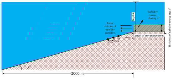
Figure 2.
Excitation wave velocity simulation model and parameters.
Table 3.
Simulation results under different variables conditions.
3.3.1. The Influence of Turbidity Current Density on the Propagation Velocity and Amplitude of Excitation Waves
The variations in surface elevation at three sensor locations in the simulated results of five different turbidity current density groups are presented in Figure 3.
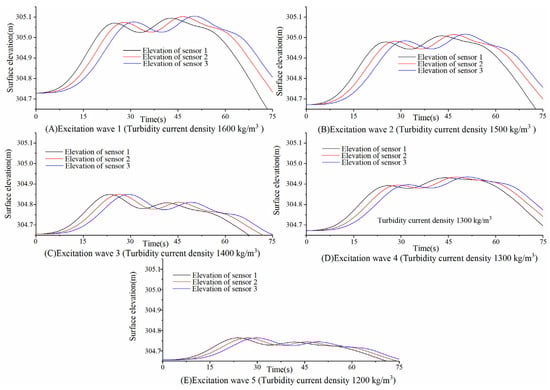
Figure 3.
Simulation of propagating velocity of excitation wave under the sole variable condition of turbulent current density. (Length of turbidity source area: 1000 m; canyon width: 200 m; thickness of turbidity source area: 20 m; depth: 200 m; initial velocity of turbidity current: 0 m/s).
Based on the simulation results described above, while keeping all other conditions constant, the impact of a single variable, namely, the turbidity current density, on the propagation velocity and amplitude of the excitation wave was analyzed. By fitting the data, the relationship between turbidity current density and the propagation velocity of turbidity currents as well as the amplitude of the excitation wave was obtained, as shown in Figure 4.
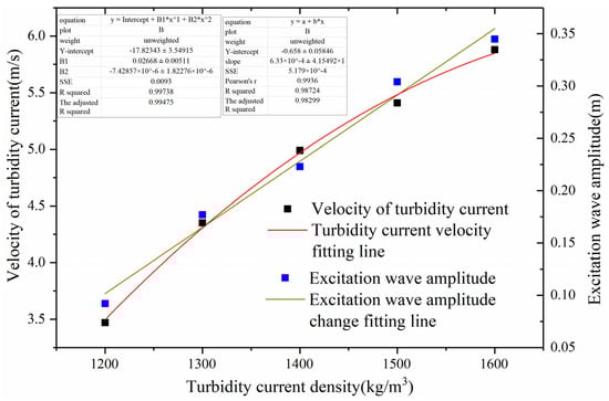
Figure 4.
Relationship between turbidity current density and turbidity current velocity, as well as excitation wave amplitude.
The simulation results indicate that changes in turbidity current density, while keeping the other conditions constant, do not result in a change in the propagation velocity of the excitation waves. However, they do affect the amplitude of the excitation waves and the velocity of the turbidity current itself. The simulation reveals that within the selected density range, both the amplitude of the excitation waves and the velocity of the turbidity current increase with increasing turbidity current density. When the turbidity current density is equal to that of water (ρTurbidity current = ρWater), there is no turbidity current or excitation wave generation. Thus, the relationship between the turbidity current velocity (v) and density (ρ) is expressed as v = −34.80643 + 0.05082•ρ − 1.59286 × 10⁻⁵ ρ2 (ρ > 1000, R2 = 0.994). Additionally, the relationship between the amplitude of the excitation waves (A) caused by turbidity currents and density (ρ) is expressed as A = −0.6021 + 5.9729 × 10⁻⁴ ρ (ρ > 1000, R2 = 0.991).
3.3.2. The Influence of the Thickness of the Turbidity Source Area on the Propagation Velocity and Amplitude of Excitation Waves
The variations in surface elevation at three sensor locations in the simulated results of five different thickness of turbidity source area groups are presented in Figure 5.
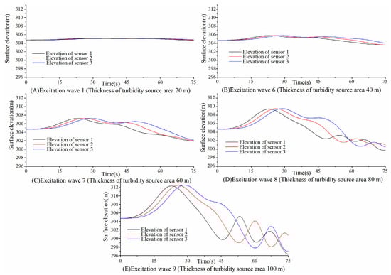
Figure 5.
Simulation of propagating velocity of excitation wave under the sole variable condition of thickness of turbidity source area. (Turbidity current density: 1600 kg/m3; length of turbidity source area: 1000 m; canyon width: 200 m; depth: 200 m; initial velocity of turbidity current: 0 m/s).
Based on the simulation results described above, while keeping all other conditions constant, the impact of a single variable, namely, the thickness of the turbidity source area, on the propagation velocity and amplitude of the excitation wave was analyzed. By fitting the data, the relationship between the thickness of the turbidity source area and the propagation velocity of the turbidity current as well as the amplitude of the excitation wave was obtained, as shown in Figure 6.
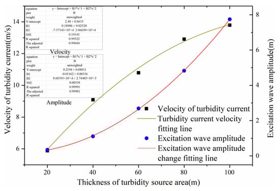
Figure 6.
Relationship between thickness of turbidity source area and turbidity current velocity, as well as excitation wave amplitude.
Based on the simulated results mentioned above, it can be concluded that, while keeping the other conditions constant, changing only the thickness of the turbidity current source area does not affect the propagation velocity of the excitation waves. However, it does impact both the amplitude of the excitation waves and the velocity of the turbidity current itself. The simulation reveals that within the selected range of thickness values for the turbidity current source area, both the amplitude of the excitation waves and the velocity of the turbidity current increase with an increase in the thickness of the source area. Additionally, it is observed that when the length of the turbidity current source area is zero, neither the turbidity current nor the excitation waves are generated (i.e., no turbidity current is produced when hTurbidity current = 0). Therefore, the relationship between the velocity (v) of the turbidity current and its thickness (h) is expressed as v = 0.27983•h − 0.00146•h2 (h ≥ 0, R2 = 0.999). Similarly, the relationship between the amplitude (A) of the excitation waves caused by the turbidity current and its thickness (h) is A = −0.00375•h − 0.0008•h2 (h ≥ 0, R2 = 0.999).
3.3.3. The Influence of the Length of the Turbidity Source Area on the Propagation Velocity and Amplitude of Excitation Waves
The variations in surface elevation at three sensor locations in the simulated results of five different length of turbidity source area groups are presented in Figure 7.
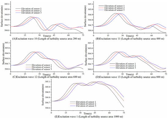
Figure 7.
Simulation of propagating velocity of excitation wave under the sole variable condition of length of turbidity source area. (Turbidity current density: 1600 kg/m3; canyon width: 200 m; thickness of turbidity source area: 20 m; depth: 200 m; initial velocity of turbidity current: 0 m/s).
Based on the simulation results described above, while keeping all other conditions constant, the impact of a single variable, namely, the length of the turbidity source area, on the propagation velocity and amplitude of the excitation wave was analyzed. By fitting the data, the relationship between the length of the turbidity source area and the amplitude of the excitation wave was obtained, as shown in Figure 8.
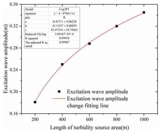
Figure 8.
Relationship between length of turbidity source area and excitation wave amplitude.(Amplitude refers to the surface elevation change caused by the excitation wave).
Through simulations, it has been determined that within the chosen range of the length of the turbidity source area, the amplitude of the excitation waves increases with an increase in the length of the turbidity source area. When the length of the turbidity source area is zero, there is no turbidity current and no generation of excitation waves (i.e., when LTurbidity current = 0). Additionally, for large lengths of the turbidity source area, under the condition of sufficient sediment supply, the variations in surface elevation caused by the waves generated by turbidity currents are negligible. Therefore, the relationship between the amplitude of the excitation waves (A) generated by turbidity currents and the length of the turbidity source area (L) is expressed as follows: A = −0.3624 + 0.10305•ln(L − 6.15619) (L ≥ 0, R2 = 0.997).
3.3.4. The Influence of Depth on the Propagation Velocity and Amplitude of Excitation Waves
The variations in surface elevation at three sensor locations in the simulated results of five different depth groups are presented in Figure 9.
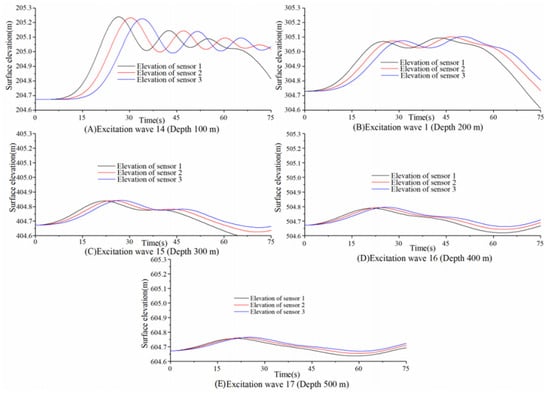
Figure 9.
Simulation of propagation velocity of excitation wave under the sole variable condition of depth. (Turbidity current density: 1600 kg/m3; length of turbidity source area: 1000 m; canyon width: 200 m; thickness of turbidity source area: 20 m; initial velocity of turbidity current: 0 m/s).
Based on the simulation results described above, while keeping all other conditions constant, the impact of a single variable, namely, depth, on the propagation velocity and amplitude of the excitation wave was analyzed. By fitting the data, the relationship between depth and the propagation velocity of the excitation wave as well as the amplitude of the excitation wave was obtained, as shown in Figure 10.
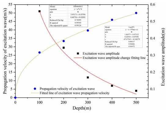
Figure 10.
Relationship between depth and propagating velocity of excitation wave, as well as excitation wave amplitude.
As the water depth approaches infinity, the excitation wave amplitude can only approach zero but cannot reach zero. Therefore, the characteristics of the excitation wave amplitude change with the water depth are similar to those of the velocity propagation of the excitation wave. The relationship between the velocity of the excitation wave induced by turbidity currents (vExcitation wave) and the water depth (H) can be described as vExcitation wave = −287.05446 + 48.59211•ln(H + 535.14863) (R2 = 0.998). The relationship between the excitation wave amplitude (A) and the water depth (H) can be expressed as A = 1.46573 − 0.22816•ln(H − 47.67563) (R2 = 0.985).
3.3.5. The Influence of the Canyon Width on the Propagation Velocity and Amplitude of Excitation Waves
The variations in surface elevation at three sensor locations in the simulated results of five different canyon width groups are presented in Figure 11.
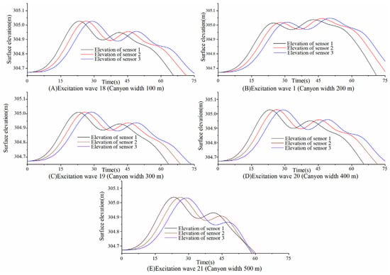
Figure 11.
Simulation of propagating velocity of excitation wave under the sole variable condition of canyon width. (Turbidity current density: 1600 kg/m3; length of turbidity source area: 1000 m; thickness of turbidity source area: 20 m; depth: 200 m; initial velocity of turbidity current: 0 m/s).
When the canyon width is taken as the single variable condition, changing the canyon width does not significantly affect the propagation velocity of excitation waves, the amplitude of excitation waves, and the velocity of turbidity currents. Therefore, it can be concluded that, without considering the impact of the differences in the terrain and sediment on the canyon width, the canyon width has no impact on the propagation of excitation waves and the movement of turbidity currents.
3.3.6. The Influence of the Initial Velocity of the Turbidity Current on the Propagation Velocity and Amplitude of Excitation Waves
The variations in surface elevation at three sensor locations in the simulated results of five different initial velocity of turbidity current groups are presented in Figure 12.
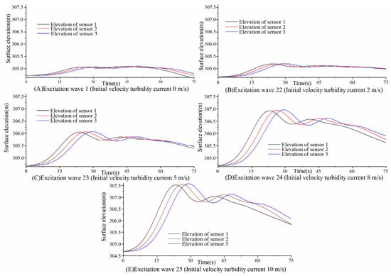
Figure 12.
Simulation of propagating velocity of excitation wave under the sole variable condition of initial velocity of turbidity current. (Turbidity current density: 1600 kg/m3; length of turbidity source area: 1000 m; canyon width: 200 m; thickness of turbidity source area: 20 m; depth: 200 m).
Based on the simulation results described above, while keeping all other conditions constant, the impact of a single variable, namely, the initial velocity of the turbidity current, on the propagation velocity and amplitude of the excitation wave was analyzed. By fitting the data, the relationship between the initial velocity of the turbidity current and the amplitude of the excitation wave was obtained, as shown in Figure 13.
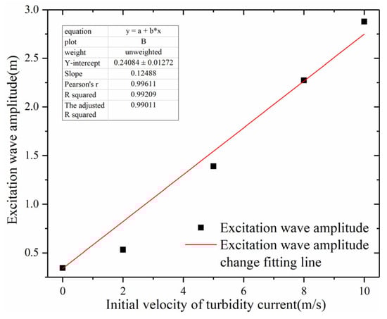
Figure 13.
Relationship between initial velocity of turbidity current and excitation wave amplitude.
Based on the simulation, it is observed that within the selected range of the initial velocity of the turbidity current, the amplitude of the excitation wave increases linearly with the increase in the initial velocity of the turbidity current. Therefore, the relationship between the amplitude (A) of the excitation wave caused by the turbidity current and the initial velocity of the turbidity current (v0) can be expressed as A = 0.34 + 0.24084•v0 (A ≥ 0, R2 = 0.992).
Through controlling the simulation calculation of a single variable, it was found that there are several factors that can affect the amplitude of the excitation wave. These factors include the turbidity current density ρ, the thickness of the turbidity current source area d, the length of the turbidity current source area L, the water depth h, and the initial velocity of the turbidity current v0. In contrast, there are relatively few factors that influence the propagation velocity of the excitation wave. Within the selected parameter range, only the water depth can affect the propagation velocity of the excitation wave. The physical parameters of the turbidity current, including the turbidity current density ρ, the thickness of the turbidity current source area d, the length of the turbidity current source area L, the canyon width l, and the initial velocity of the turbidity current v0, have no direct influence on the propagation velocity of the excitation wave. Therefore, the turbidity current only serves as a triggering factor for the excitation wave and is not directly related to the propagation velocity of the excitation wave.
3.4. Analyze the Changes in Propagation Velocity of Excitation Waves along a Path
In order to further investigate the underlying truth behind the variation in the propagation velocity of the excitation wave, a discussion on whether there is velocity attenuation along the propagation path of the excitation wave is conducted. Since the seventh group of the excitation wave causes significant changes in surface elevation, the seventh group of the excitation wave is selected as the research object in order to study the variations in surface elevation along the propagation path of the excitation wave. The changes in surface elevation are extracted every 200 m along the sediment slope (with the first extraction point located 400 m away from the source area of the turbidity current). A total of six sets of surface elevation data are extracted (ranging from 400 m to 1400 m distance from the source area of the turbidity current), as shown in Figure 14.
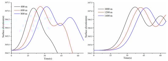
Figure 14.
Surface elevation changes during excitation wave propagation along sediment slopes.
The amplitudes and propagation velocities of the excitation wave at each point are shown in Table 4.
Table 4.
Excitation wave velocity during the excitation wave propagation along the sediment slope.
From the table above, it can be observed that the amplitude of the excitation wave does not change while traveling along the slope. This indicates that the change in surface elevation caused by the propagation of the excitation wave does not attenuate. Furthermore, the propagation velocity of the excitation wave gradually increases, although the change is not very pronounced. This variation may be attributed to the change in the water depth caused by the sloping bed. To investigate this, a simulation was conducted in a straight channel with a length of 3000 m. Six sampling points were established from 400 m to 1400 m away from the turbidity current source area to extract the amplitude of the excitation wave. The results of the simulation are presented in Figure 15.
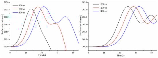
Figure 15.
Surface elevation changes during wave propagation along a straight channel.
The amplitudes and propagation velocities of the excitation wave at each point are shown in Table 5.
Table 5.
Excitation wave velocity during the propagation along the straight channel.
The data from the table above indicate that during the propagation of the excitation wave along a straight water channel, its velocity remains constant, except for a slight decrease at the initial point. This phenomenon may be attributed to the fact that in the starting phase, the excitation wave is not fully developed, and hence its velocity is relatively smaller. However, once it is fully developed, the propagation velocity of the excitation wave does not decrease in subsequent processes. Therefore, the propagation velocity of the excitation wave is only dependent on the real-time water depth of the wave. In future studies, we aim to explore the relationships between these influencing factors and other physical parameters, such as the speed of wave propagation, using the effective and accurate method of machine learning algorithms [45].
3.5. Expression of the Propagation Velocity of the Excitation Wave
The propagation of the excitation wave along a long distance does not experience an attenuation in velocity, as is the case with the propagation velocity of solitary waves. Referring to the estimated wave propagation velocity (the square of the propagation velocity is directly proportional to the water depth amplitude) [46], the wavelengths under different water depth conditions were extracted, as shown in Table 6.
Table 6.
Physical parameters of excitation wave under different water depth conditions.
From the simulation results of a single variable, the water depth, it could be seen that the wavelengths of the excitation waves were much larger than the water depth. Therefore, further simulations were conducted under water depth conditions ranging from 1000 m to 4000 m. Due to the minimal change in wave amplitude when the water depth reached 4000 m, it was not possible to observe a distinct waveform. However, through simulations with the thickness of the turbidity current source area as the single variable, it was found that an increase in the thickness of the source region led to a larger amplitude of the excitation waves, but it did not affect the wavelength of the excitation waves. Therefore, in order to better extract the wavelength of the excitation waves, the thickness of the source region in the simulation with a water depth of 4000 m was set to 200 m.
Through simulations at water depths of 1000 m and 4000 m, it is observed that the wavelengths of the excitation waves are much larger than the water depth, indicating that these waves belong to the category of shallow water waves. The amplitude of the excitation waves is relatively small compared to their wavelength, aligning with the small amplitude wave theory [47]. According to this theory, the wave velocity of shallow water waves is only dependent on the water depth (h) and gravity acceleration (g), regardless of the wave period. In the case of excitation waves induced by turbidity currents in deep water, the amplitudes of these waves are relatively small compared to the water depth. Referring to the expression for shallow water waves (when the relative water depth, which is the ratio of water depth to wavelength, is much smaller than 1/2), the wave velocity is denoted as ‘’. This implies that the propagation velocity of the excitation waves is also solely related to the water depth. Therefore, a fitting of the square of the propagation velocity of the excitation waves (v2) and the water depth (h) was conducted (Figure 16).
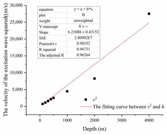
Figure 16.
The relationship between the propagation velocity of excitation wave and the depth.
Through fitting, the following can be obtained:
Through fitting, it can be discovered that the propagation model of the velocity of excitation waves is different from the shallow water wave theory. This is because turbidity currents, as granular materials, generate excitation waves by pushing the water in front of them with sediment particles underwater, which is different from the surges formed by solid blocks entering the ocean. Additionally, excitation waves formed by turbidity currents occur in an underwater environment, which may be the reason why the propagation velocity equation for the excitation waves behaves as if the velocity squared is equal to half the Earth’s gravity. This equation reveals the variation in the propagation velocity of the excitation wave with depth, explaining why the average velocity between the monitoring points in the field is greater than the instantaneous velocity measured at these points [41]. Further theoretical research on the propagation velocity of excitation waves requires subsequent field monitoring and the deployment of monitoring systems to more thoroughly investigate the fundamental causes.
4. Conclusions
This study aimed to investigate the velocity of turbidity current-induced excitation waves through numerical simulation. By fixing a single variable, different factors that could affect the propagation velocity and amplitude of the excitation waves were analyzed and discussed, leading to the following three conclusions:
- Within the selected parameter range, there are several factors that can influence the amplitude of the excitation waves, including the turbidity current density ρ, the thickness of the turbidity current source area d, the length of the turbidity current source area L, the water depth h, and the initial velocity of the turbidity current v0.The amplitude of the excitation waves is positively correlated with the turbidity density, the thickness of the source area, the length of the source area, and the initial velocity, while it is negatively correlated with the water depth.
- Within the selected parameter range, only the water depth can affect the propagation velocity of the excitation waves. As the water depth increases, the propagation velocity of the excitation waves also increases, and a relationship of v2 = 0.63gh (R2 = 0.967) is established between the square of the propagation velocity v2 and the water depth h.
- During the propagation of the excitation waves, both the propagation velocity and the changes in surface elevation caused by the waves do not attenuate. Considering the relatively calm deep-sea environment, the high-speed propagation of the excitation waves and the resuspension of bottom sediments they cause not only complement the understanding of turbidity current motion patterns in canyons, but also provide new research directions for deep-sea sediment transport.
Author Contributions
Conceptualization and methodology, G.X., S.S. and Y.R.; formal analysis, Z.C. and Y.R.; data curation, S.S. and M.L.; writing—original draft preparation, S.S. and G.X.; writing—review and editing, S.S. and G.X.; visualization, Y.R. and M.L.; project administration, G.X.; funding acquisition, G.X. All authors have read and agreed to the published version of the manuscript.
Funding
The project is supported by the National Natural Science Foundation of China (Grant Nos. 42206055 and 41976049).
Institutional Review Board Statement
Not applicable.
Informed Consent Statement
Not applicable.
Data Availability Statement
The data presented in this study are available on request from the corresponding author.
Acknowledgments
The author would like to thank Yang Li for his help with the work.
Conflicts of Interest
The authors declare no conflicts of interest.
References
- Azpiroz-Zabala, M.; Cartigny, M.J.B.; Talling, P.J.; Parsons, D.R.; Sumner, E.J.; Clare, M.A.; Simmons, S.M.; Cooper, C.; Pope, E.L. Newly recognized turbidity current structure can explain prolonged flushing of submarine canyons. Sci. Adv. 2017, 3, e1700200. [Google Scholar] [CrossRef] [PubMed]
- Daly, R.A. Origin of submarine canyons. Am. J. Sci. 1936, 5, 401–420. [Google Scholar] [CrossRef]
- Winterwerp, J. Stratification effects by fine suspended sediment at low, medium, and very high concentrations. J. Geophys. Res. Oceans. 2006, 111, C5. [Google Scholar] [CrossRef]
- Nilsen, T.H.; Shew, R.D.; Steffens, G.S.; Studlick, J.R.J. Atlas of Deep-Water Outcrops; American Association of Petroleum Geologists: Tulsa, OK, USA, 2008. [Google Scholar] [CrossRef]
- Xu, J. Turbidity Current Research in the Past Century: An Overview. J. Ocean Univ. China 2014, 44, 98–105. [Google Scholar] [CrossRef]
- Talling, P.J.; Allin, J.; Armitage, D.A.; Arnott, R.W.C.; Cartigny, M.J.B.; Clare, M.A.; Felletti, F.; Covault, J.A.; Girardclos, S.; Hansen, E.; et al. Key future directions for research on turbidity currents and their deposits. J. Sediment. Res. 2015, 85, 153–169. [Google Scholar] [CrossRef]
- Maier, K.L.; Gales, J.A.; Paull, C.K.; Rosenberger, K.; Talling, P.J.; Simmons, S.M.; Gwiazda, R.; McGann, M.; Cartigny, M.J.; Lundsten, E. Linking direct measurements of turbidity currents to submarine canyon-floor deposits. Front. Earth Sci. 2019, 7, 144. [Google Scholar] [CrossRef]
- Hughes Clarke, J.E. First wide-angle view of channelized turbidity currents links migrating cyclic steps to flow characteristics. Nat. Commun. 2016, 7, 11896. [Google Scholar] [CrossRef]
- Normandeau, A.; Bourgault, D.; Neumeier, U.; Lajeunesse, P.; St-Onge, G.; Gostiaux, L.; Chavanne, C. Storm-induced turbidity currents on a sediment-starved shelf: Insight from direct monitoring and repeat seabed mapping of upslope migrating bedforms. Sedimentology 2020, 67, 1045–1068. [Google Scholar] [CrossRef]
- Hill, P.R.; Lintern, D.G. Turbidity currents on the open slope of the Fraser Delta. Mar. Geol. 2022, 445, 106738. [Google Scholar] [CrossRef]
- Summers, M. Review of deep-water submarine cable design. In Proceedings of the SubOptic 2001, Kyoto, Japan, 20–24 May 2001; p. 4. [Google Scholar]
- Carter, L.; Gavey, R.; Talling, P.J.; Liu, J.T. Insights into Submarine Geohazards from Breaks in Subsea Telecommunication Cables. Oceanography 2014, 27, 58–67. [Google Scholar] [CrossRef]
- Gavey, R.; Carter, L.; Liu, J.T.; Talling, P.J.; Hsu, R.; Pope, E.; Evans, G. Frequent sediment density flows during 2006 to 2015, triggered by competing seismic and weather events: Observations from subsea cable breaks off southern Taiwan. Mar. Geol. 2017, 384, 147–158. [Google Scholar] [CrossRef]
- Carter, L.; Burnett, D.; Drew, S.; Hagadorn, L.; Marle, G.; Bartlett-Mcneil, D.; Irvine, N. Submarine Cables and the Oceans: Connecting the World; UNEP-WCMC Biodiversity Series 31; UNEP World Conservation Monitoring Centre: Cambridge, UK, 2010. [Google Scholar]
- Qiu, W. Submarine cables cut after Taiwan earthquake in Dec 2006. Submar. Cable Netw. 2011, 19. [Google Scholar]
- Heezen, B.C.; Ewing, W.M. Turbidity currents and submarine slumps, and the 1929 Grand Banks [Newfoundland] earthquake. Am. J. Sci. 1952, 250, 849–873. [Google Scholar] [CrossRef]
- Kuenen, P.H. Estimated size of the Grand Banks [Newfoundland] turbidity current. Am. J. Sci. 1952, 250, 874–884. [Google Scholar] [CrossRef]
- Heezen, B.C.; Ericson, D.; Ewing, M. Further evidence for a turbidity current following the 1929 Grand Banks earthquake. Deep-Sea Res. 1954, 1, 193–202. [Google Scholar] [CrossRef]
- Heezen, B.C. Whales entangled in deep sea cables. Deep-Sea Res. 1957, 4, 105–115. [Google Scholar] [CrossRef]
- Piper, D.J.; Shor, A.N.; Farre, J.A.; O’Connell, S.; Jacobi, R. Sediment slides and turbidity currents on the Laurentian Fan: Sidescan sonar investigations near the epicenter of the 1929 Grand Banks earthquake. Geology 1985, 13, 538–541. [Google Scholar] [CrossRef]
- Piper, D.J.; Cochonat, P.; Morrison, M.L. The sequence of events around the epicentre of the 1929 Grand Banks earthquake: Initiation of debris flows and turbidity current inferred from sidescan sonar. Sedimentology 1999, 46, 79–97. [Google Scholar] [CrossRef]
- Houtz, R.; Wellman, H. Turbidity current at Kadavu Passage, Fiji. Geol. Mag. 1962, 99, 57–62. [Google Scholar] [CrossRef]
- Heezen, B.C.; Ewing, M. Orleansville earthquake and turbidity currents. AAPG Bull. 1955, 39, 2505–2514. [Google Scholar] [CrossRef]
- Krause, D.C.; White, W.C.; PIPER, D.J.W.; Heezen, B.C. Turbidity currents and cable breaks in the western New Britain Trench. Geol. Soc. Am. Bull. 1970, 81, 2153–2160. [Google Scholar] [CrossRef]
- Piper, D.J.; Savoye, B. Processes of late Quaternary turbidity current flow and deposition on the Var deep-sea fan, north-west Mediterranean Sea. Sedimentology 1993, 40, 557–582. [Google Scholar] [CrossRef]
- Soh, W.; Machiyama, H.; Shirasaki, Y.; Kasahara, J. Deep-sea floor instability as a cause of deepwater cable fault, off eastern part of Taiwan. AGU Fall Meet. Abstr. 2004, 2, 1–8. [Google Scholar]
- Cattaneo, A.; Babonneau, N.; Ratzov, G.; Dan-Unterseh, G.; Yelles, K.; Bracène, R.; De Lepinay, B.M.; Boudiaf, A.; Déverchère, J. Searching for the seafloor signature of the 21 May 2003 Boumerdès earthquake offshore central Algeria. Nat. Hazards Earth Syst. Sci. 2012, 12, 2159–2172. [Google Scholar] [CrossRef]
- Hsu, S.-K.; Kuo, J.; Chung-Liang, L.; Ching-Hui, T.; Doo, W.-B.; Ku, C.-Y.; Sibuet, J.-C. Turbidity currents, submarine landslides and the 2006 Pingtung earthquake off SW Taiwan. Terr. Atmos. Ocean. Sci. 2008, 19, 7. [Google Scholar] [CrossRef]
- Carter, L.; Milliman, J.D.; Talling, P.J.; Gavey, R.; Wynn, R.B. Near-synchronous and delayed initiation of long run-out submarine sediment flows from a record-breaking river flood, offshore Taiwan. Geophys. Res. Lett. 2012, 39, L12603. [Google Scholar] [CrossRef]
- Clare, M.A.; Yeo, I.A.; Watson, S.; Wysoczanski, R.; Seabrook, S.; Mackay, K.; Hunt, J.E.; Lane, E.; Talling, P.J.; Pope, E.; et al. Fast and destructive density currents created by ocean-entering volcanic eruptions. Science 2023, 381, 1085–1092. [Google Scholar]
- Ren, Y.; Zhang, Y.; Xu, G.; Xu, X.; Wang, H.; Chen, Z. The failure propagation of weakly stable sediment: A reason for the formation of high-velocity turbidity currents in submarine canyons. J. Ocean. Limnol. 2023, 41, 100–117. [Google Scholar] [CrossRef]
- Wang, Z.; Xu, J.; Talling, P.J.; Cartigny, M.J.B.; Simmons, S.M.; Gwiazda, R.; Paull, C.K.; Maier, K.L.; Parsons, D.R. Direct evidence of a high-concentration basal layer in a submarine turbidity current. Deep-Sea Res. Part I Oceanogr. Res. Pap. 2020, 161, 103300. [Google Scholar] [CrossRef]
- Ren, Y.; Tian, H.; Chen, Z.; Xu, G.; Liu, L.; Li, Y. Two Kinds of Waves Causing the Resuspension of Deep-Sea Sediments: Excitation and Internal Solitary Waves. J. Ocean Univ. China 2023, 22, 429–440. [Google Scholar] [CrossRef]
- Lambert, A.M.; Kelts, K.R.; Marshall, N.F. Measurements of density underflows from Walensee, Switzerland. Sedimentology 1976, 23, 87–105. [Google Scholar] [CrossRef]
- Piper, D.J.W.; Shor, A.N.; Hughes Clarke, J.E. The 1929 “Grand Banks” earthquake, slump, and turbidity current. In Sedimentologic Consequences of Convulsive Geologic Events; Geological Society of America: Boulder, CO, USA, 1988; pp. 77–92. [Google Scholar] [CrossRef]
- Paull, C.K.; Talling, P.J.; Maier, K.L.; Parsons, D.; Xu, J.; Caress, D.W.; Gwiazda, R.; Lundsten, E.M.; Anderson, K.; Barry, J.P. Powerful turbidity currents driven by dense basal layers. Nat. Commun. 2018, 9, 4114. [Google Scholar] [CrossRef] [PubMed]
- Ren, Y.; Zhou, H.; Wang, H.; Wu, X.; Xu, G.; Meng, Q. Study on the critical sediment concentration determining the optimal transport capability of submarine sediment flows with different particle size composition. Mar. Geol. 2023, 464, 107142. [Google Scholar] [CrossRef]
- Bagnold, R.A. Auto-suspension of transported sediment; turbidity currents. Proc. R. Soc. Lond. Ser. A Math. Phys. Sci. 1962, 265, 315–319. [Google Scholar]
- Parker, G. Conditions for the ignition of catastrophically erosive turbidity currents. Mar. Geol. 2003, 46, 307–327. [Google Scholar] [CrossRef]
- Pantin, H.M. Interaction between velocity and effective density in turbidity flow: Phase-plane analysis, with criteria for autosuspension. Mar. Geol. 1979, 31, 59–99. [Google Scholar] [CrossRef]
- Heerema, C.J.; Talling, P.J.; Cartigny, M.J.; Paull, C.K.; Bailey, L.; Simmons, S.M.; Parsons, D.R.; Clare, M.A.; Gwiazda, R.; Lundsten, E.; et al. What determines the downstream evolution of turbidity currents? Earth Planet. Sci. Lett. 2020, 532, 116023. [Google Scholar] [CrossRef]
- Talling, P.J.; Cartigny, M.J.B.; Pope, E.; Baker, M.; Clare, M.A.; Heijnen, M.; Hage, S.; Parsons, D.R.; Simmons, S.M.; Paull, C.K.; et al. Detailed monitoring reveals the nature of submarine turbidity currents. Nat. Rev. Earth Environ. 2023, 4, 642–658. [Google Scholar] [CrossRef]
- Heimsund, S. Numerical Simulation of Turbidity Currents: A New Perspective for Small-and Large-Scale Sedimentological Experiments; Sedimentology/Petroleum Geology; University of Bergen: Bergen, Norway, 2007. [Google Scholar]
- Zhou, J.; Cenedese, C.; Williams, T.; Ball, M.; Venayagamoorthy, S.K.; Nokes, R.I. On the Propagation of Gravity Currents Over and through a Submerged Array of Circular Cylinders. J. Fluid Mech. 2017, 831, 394–417. [Google Scholar] [CrossRef]
- Saha, S.; De, S.; Changdar, S. An Application of Machine Learning Algorithms on the Prediction of the Damage Level of Rubble-Mound Breakwaters. J. Offshore Mech. Arct. Eng. 2024, 146, 011202. [Google Scholar] [CrossRef]
- Russell, J.S. Report on Waves: Made to the Meetings of the British Association; Richard and John E Taylor: London, UK, 1845. [Google Scholar]
- Airy, G.B. Tides and Waves; B. Fellowes: London, UK, 1845. [Google Scholar]
Disclaimer/Publisher’s Note: The statements, opinions and data contained in all publications are solely those of the individual author(s) and contributor(s) and not of MDPI and/or the editor(s). MDPI and/or the editor(s) disclaim responsibility for any injury to people or property resulting from any ideas, methods, instructions or products referred to in the content. |
© 2024 by the authors. Licensee MDPI, Basel, Switzerland. This article is an open access article distributed under the terms and conditions of the Creative Commons Attribution (CC BY) license (https://creativecommons.org/licenses/by/4.0/).