
A New Method and Model for the Estimation of Residual Value of Agricultural Tractors


Abstract
:1. Introduction
1.1. Previous Studies
1.2. Current Issues
1.3. Goal
2. Materials and Methods
2.1. Dataset
2.2. Data Systematization and Preprocessing
2.2.1. New Equivalent Tractor
2.2.2. Tractor Family
2.3. Data Analysis
3. Results
3.1. Proposed Regression Models
3.2. Fitted Regression Models with Multiple Variables and Validations
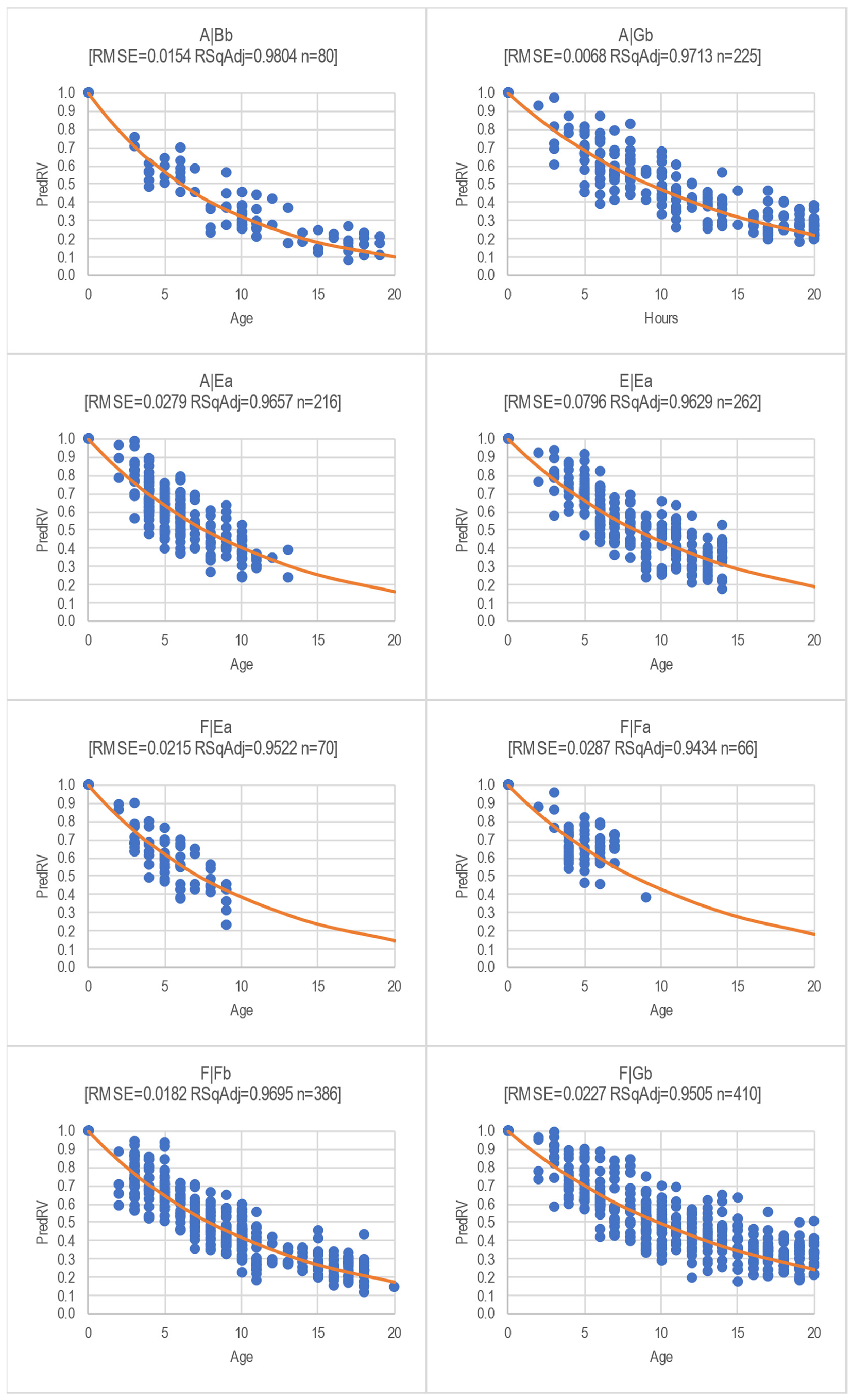
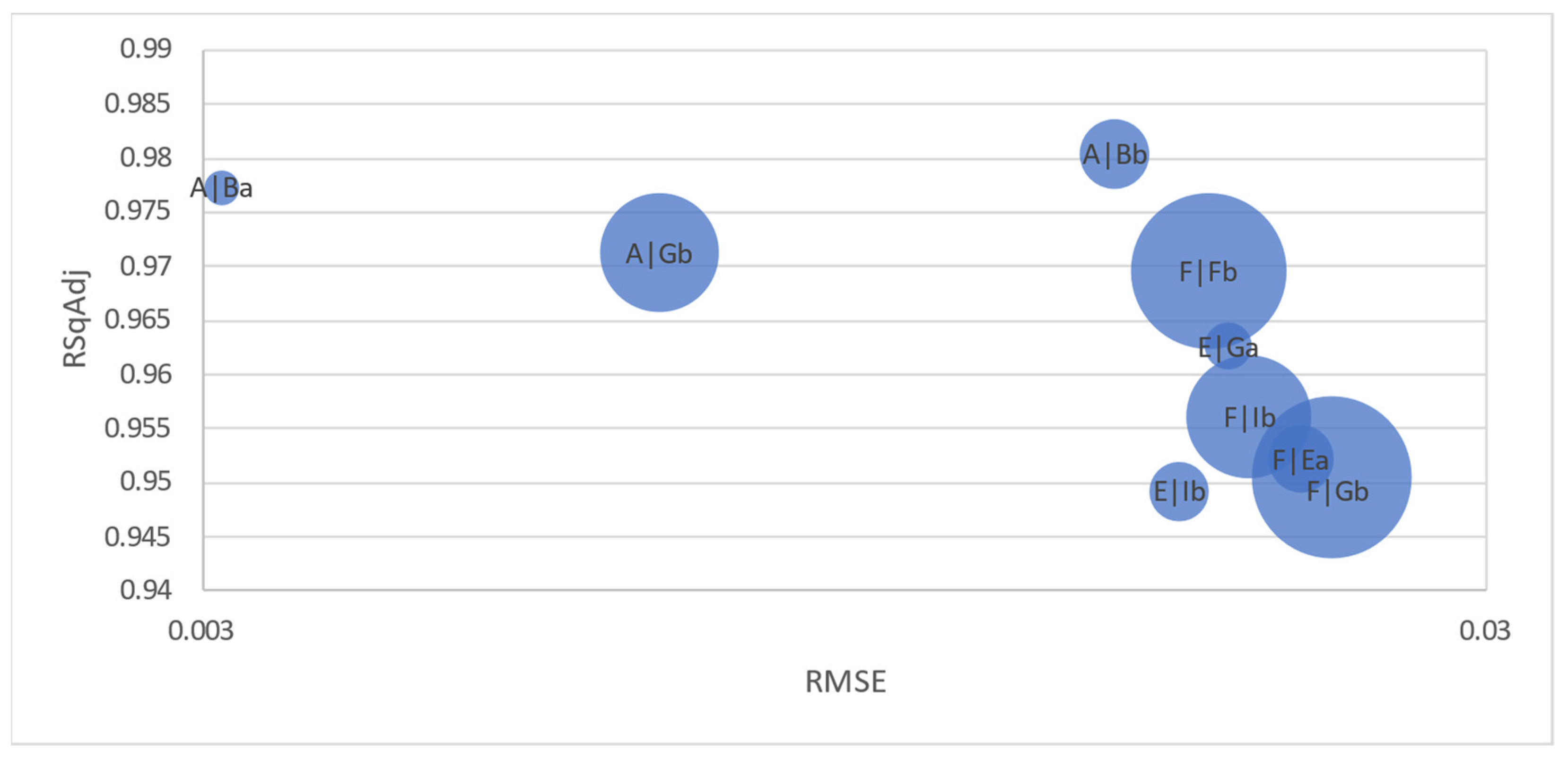
3.3. Fitted Regression Models of Tractor Families
4. Discussion
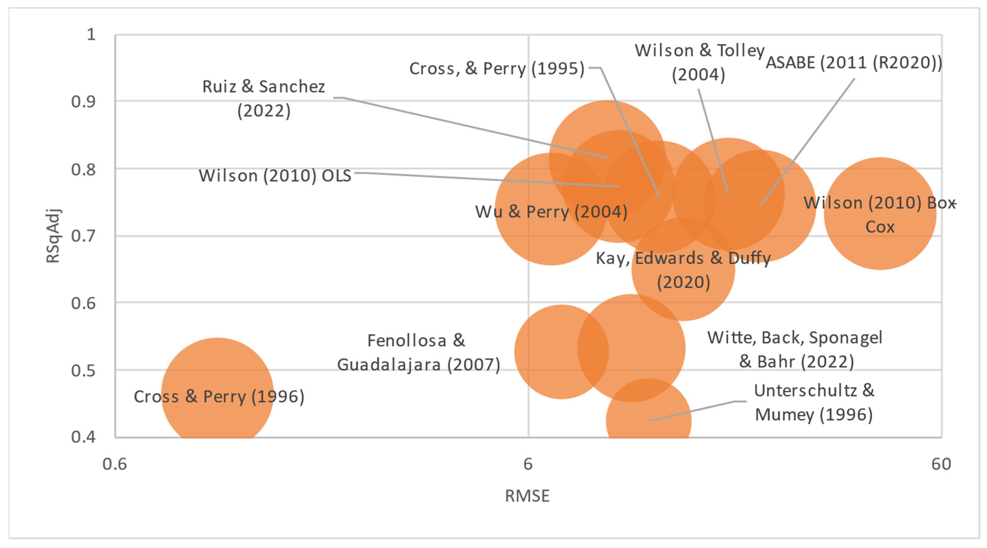
4.1. Models Referenced by Previous Studies
4.2. General
5. Conclusions
Author Contributions
Funding
Institutional Review Board Statement
Informed Consent Statement
Data Availability Statement
Acknowledgments
Conflicts of Interest
References
- Kastens, T. Farm Machinery Operations Cost Calculations; Kansas State University, Agricultural Experiment Station and Cooperative Extension Service: Manhattan, KS, USA, 1997. [Google Scholar]
- Edwards, W. Replacement Strategies for Farm Machinery; Iowa State University: Ames, IA, USA, 2019. [Google Scholar]
- U.S. Consumer Financial Protection Bureau. What Is a Loan to Value Ratio and How Does It Relate to My Costs. Available online: https://www.consumerfinance.gov/ask-cfpb/what-is-a-loan-to-value-ratio-and-how-does-it-relate-to-my-costs-en-121/#:~:text=The%20loan%2Dto%2Dvalue%20(,will%20require%20private%20mortgage%20insurance (accessed on 1 January 2023).
- ECB. Haircuts. Available online: https://www.ecb.europa.eu/ecb/educational/explainers/tell-me-more/html/haircuts.en.html (accessed on 1 January 2023).
- Renius, K.T. Fundamentals of Tractor Design; Springer: Cham, Switzerland, 2020. [Google Scholar]
- Peacock, D.L.; Brake, J.R. What Is Used Farm Machinery Worth? Agricultural Experiment Station East Lansing; Department of Agricultural Economics, Michigan State University: East Lansing, MI, USA, 1970. [Google Scholar]
- Veen, H.; Meulen, H.; Bommel, K.; Doorneweert, B. Exploring Agricultural Taxation in Europe; LEI: The Hague, The Netherlands, 2007. [Google Scholar]
- Reid, D.W.; Bradford, G.L. On Optimal Replacement of Farm Tractors. Am. J. Agric. Econ. 1983, 65, 326–331. [Google Scholar] [CrossRef]
- Musser, W.N.; Tew, B.V.; White, F.C. Choice of Depreciation Methods for Farm Firms. Am. J. Agric. Econ. 1986, 68, 980–989. [Google Scholar]
- Weersink, A.; Stauber, S. Optimal Replacement Intercal and Depreciation Method for a Grain Combine. West. J. Agric. Econ. 1988, 13, 18–28. [Google Scholar]
- Cross, T.L.; Perry, G.M. Depreciation Patterns for Agricultural Machinery. Am. J. Agric. Econ. 1995, 77, 194–204. [Google Scholar] [CrossRef]
- Cross, T.; Perry, G. Remaining Value Functions for Farm Equipment. Appl. Eng. Agric. 1996, 12, 547–553. [Google Scholar] [CrossRef]
- Unterschultz, J.; Mumey, G. Reducing Investment Risk in Tractors and Combines with Improved Terminal Asset Value Forecasts. Can. J. Agric. Econ./Rev. Can. D’agroeconomie 1996, 44, 295–309. [Google Scholar]
- Dumler, T.J.; Burton, R.O.; Kastens, T.L. Use of Alternative Depreciation Methods to Estimate Farm Tractor Values. In Proceedings of the Selected Paper at the AAEA Annual Meeting, Tampa, FL, USA, 30 July–2 August 2000; pp. 30–32. [Google Scholar]
- Dumler, T.J.; Burton, R.O.; Kastens, T.L. Predicting Farm Tractor Values through Alternative Depreciation Methods. Rev. Agric. Econ. 2003, 25, 506–522. [Google Scholar]
- Wu, J.; Perry, G.M. Estimating Farm Equipment Depreciation: Which Functional Form Is Best? Am. J. Agric. Econ. 2004, 86, 483–491. [Google Scholar] [CrossRef]
- ASAE Standard D497.7; ASABE Agricultural Machinery Management Data. American Society of Agricultural and Biological Engineers: Joseph, MI, USA, 2020.
- Kay, R.D.; Edwards, W.M.; Duffy, P.A. Farm Management, 7th ed.; McGraw-Hill: New York, NY, USA, 2020. [Google Scholar]
- Williams, N.T. Appropriate Rates of Depreciation for Machinery in Current Cost Accounting. Farm Manag. 1981, 4, 171–176. [Google Scholar]
- Cunningham, S.; Turner, M.M. Actual Depreciation Rates of Farm Machinery. Farm Manag. 1988, 6, 381–387. [Google Scholar]
- Wilson, P.; Davis, S. Estimating Depreciation in Tractors in the UK and Implications for Farm Management Decision Making. Farm Manag. 1998, 10, 183–193. [Google Scholar]
- Wilson, P.; Tolley, C. Estimating Tractor Depreciation and Implications for Farm Management Accounting. J. Farm Manag. 2004, 12, 5–16. [Google Scholar]
- Wilson, P. Estimating Tractor Depreciation: The Impact of Choice of Functional Form. J. Farm Manag. 2010, 13, 799–818. [Google Scholar]
- McNeill, R.C. Depreciation of Farm Tractors in British Columbia. Can. J. Agric. Econ./Rev. Can. D’agroeconomie 1979, 27, 53–58. [Google Scholar] [CrossRef]
- Hansen, L.; Lee, H. Estimating Farm Tractor Depreciation: Tax Implications. Can. J. Agric. Econ./Rev. Can. D’agroeconomie 1991, 39, 463–479. [Google Scholar] [CrossRef]
- Witte, F.; Back, H.; Sponagel, C.; Bahrs, E. Remaining Value Development of Tractors—A Call for the Application of a Differentiated Market Value Estimation. Agric. Eng. 2022, 77, 1–20. [Google Scholar] [CrossRef]
- Fenollosa, M.; Guadalajara, N. An Empirical Depreciation Model for Agricultural Tractors in Spain. Span. J. Agric. Res. 2007, 5, 130–141. [Google Scholar] [CrossRef]
- Ruiz-Garcia, L.; Sanchez-Guerrero, P. A Decision Support Tool for Buying Farm Tractors, Based on Predictive Analytics. Agriculture 2022, 12, 331. [Google Scholar] [CrossRef]
- ACEA. Economic and Market Report. State of the EU Auto Industry. Full-Year 2021; European Automobile Manufacturers’ Association (ACEA): Brussels, Belgium, 2022. [Google Scholar]
- EC. Directive 97/68/EC of the European Parliament and of the Council of 16 December 1997; European Commission (EC): Brussels, Belgium, 1997.
- EC. Directive 2000/25/EC of the European Parliament; European Commission (EC): Brussels, Belgium, 2000.
- EC. Directive 2004/26/EC of the European Parliament and of the Council of 21 April 2004 Amending Directive 97/68/EC; European Commission (EC): Brussels, Belgium, 2004.
- EC. Directive 2009/30/EC of the European Parliament and of the Council of 23 April 2009 Amending Directive 98/70/EC; European Commission (EC): Brussels, Belgium, 2009.
- Posada, F.; Chambliss, S.; Blumberg, K. Cost of Emission Reduction Technologies for Heavy Duty Diesel Vehicles; The International Council on Clean Transportation: Washington, DC, USA, 2016. [Google Scholar]
- Lynch, L.A.; Hunter, C.A.; Zigler, B.T.; Thomton, M.J.; Reznicek, E.P. On-Road Heavy-Duty Low-NOx Technology Cost Study; National Renewable Energy Laboratory (NREL), U.S. Department of Energy: Golden, CO, USA, 2020.
- Posada, F.; Isenstadt, A.; Badshah, H. Estimated Cost of a Diesel Emissions-Control Technology to Meet Future California Low NOx Standards in 2024 and 2027; The International Council of Clean Transportation: Washington, DC, USA, 2020. [Google Scholar]
- CEMA. Economic Press Release Tractor Registrations 2021; CEMA—European Agricultural Machinery: Brussels, Belgium, 2022. [Google Scholar]
- McCarthy, R.V.; McCarthy, M.M.; Ceccucci, W.; Halawi, L. Applying Predictive Analytics; Springer International Publishing: Cham, Switzerland, 2019. [Google Scholar]


| Reference | Data Source | Data Size | Variables | Function |
|---|---|---|---|---|
| Peacock, D. L., and Brake, J. R. (1970). | U.S.A. Sales | - | Age | Linear |
| ASAE (1979). | U.S.A. | - | Age | Exponential |
| McNeill, R. C. (1979). | Canada | 32 | Age and state | Exponential |
| Leatham, D. J., and Baker, T. G. (1981). | U.S.A. | 1454 tractors | Age, power, motor type, traction, and manufacturer | Exponential |
| Reid, D. W., and Bradford, G. L. (1983). | U.S.A. | 411 | Age, power, motor type, manufacturer, increasing usage, and technological changes | Exponential |
| Perry, G. M., Bayaner, A., and Nixon, C. J. (1986). | U.S.A. | 1612 | Age, power, manufacturer, usage, care, and macroeconomic variables | Box–Cox |
| Hansen, L., and Lee, H. (1991). | Canada | - | Age, year of manufacture, and purchase year | Linear |
| Cross, T. L., and Perry, G. M. (1995). | U.S.A. Auctions | - | Age, usage, manufacturer, care, type of auction, region, and macroeconomic variables | Box–Cox |
| Unterschultz, J., and Mumey, G. (1996). | U.S.A. and Canadian Auctions | 3202 Tractors | Age, manufacturer | Ratified by Hansen and Lee model |
| Cross, T. L., and Perry, G. M. (1996). | U.S.A. Auctions | 433 <60 kW 1946 60–112 kW 866 >112 kW | Age, usage, manufacturer, care, and macroeconomic variables | Box–Cox |
| Wu, J., and Perry, G. M. (2004). | U.S.A. Auctions | 657 30–79 hp 1420 80–120 hp 781 121+ hp | Age, production year, manufacturer, and other | Box–Cox |
| Fenollosa Ribera, M. L., and Guadalajara Olmeda, N. (2007). | E.S. Sales | 7876 13–79 hp 3963 80–133 hp 731 134–263 hp Dec’99-Dec’02 | Age, power, brand, and others | Ordinary Least Squares (OLS) |
| Wilson, P., and Tolley, C. (2004). | U.K. Adverts | 968 | Age, hours, power, brand, and others | Ordinary Least Squares (OLS) |
| Wilson, P. (2010). | U.K. Adverts | 1223 | Age, hours, power, brand, and others | Ordinary Least Squares (OLS) Box–Cox |
| ASABE. (2011 (R2020)). | U.S.A. | - | Age, usage, and power | Box–Cox |
| Kay, R. D., Edwards, W. M., and Duffy, P. A. (2020). | U.S.A. Auctions. | - | Based on ASABE standards, 2006 | Box–Cox |
| Witte, F., Back, H., Sponagel, C., and Bahrs, E. (2022) | German Adverts and Auctions | 2667 tractors | Age, hours, power, and brand | Exponential |
| Ruiz-Garcia, L., and Sanchez-Guerrero, P. (2022). | EUR Adverts | 227 new 1003 used | Age, hours, power, and brand | Robust linear (polynomic) |
| Model Identifier | B|Hb|006 * | B|Gb|005 * | B|Ga|005 * | B|Eb|001 * | B|Ea|001 * |
|---|---|---|---|---|---|
| Rated Power | 107 kW | ||||
| Wheelbase | 2525 mm | 2564 mm | 2820 mm | ||
| Shipping Mass | 5300 kg | 6940 kg | 7470 kg | ||
| Max Mass | 9000 kg | 10,250 kg | 10,250 kg | ||
| Transmission | Partial Powershift Transmission | Partial Powershift Transmission | Continuous Variable Transmission | Partial Powershift Transmission | Continuous Variable Transmission |
| MSRP relative to the most economical offering | |||||
| Classic Interface | 1.00 | ||||
| Advanced Interface | 1.05 | 1.13 | 1.11 | ||
| Premium Interface | 1.14 | 1.17 | 1.28 | 1.16 | 1.34 |
| Ultimate Interface | 1.22 | 1.33 | 1.21 | 1.39 | |
| Country | (<100 kW) | (100–120 kW) | (120–160 kW) | (>160 kW) | Total |
|---|---|---|---|---|---|
| Austria | 77 | 28 | 19 | 32 | 156 |
| Belgium | 12 | 24 | 59 | 52 | 147 |
| Denmark | 105 | 92 | 126 | 183 | 506 |
| Estonia | 7 | 9 | 20 | 38 | 74 |
| Finland | 117 | 83 | 58 | 15 | 273 |
| France | 1097 | 773 | 992 | 444 | 3306 |
| Germany | 459 | 420 | 838 | 1132 | 2849 |
| Italy | 65 | 35 | 39 | 66 | 205 |
| Latvia | 7 | 6 | 7 | 22 | 42 |
| Lithuania | 34 | 24 | 25 | 85 | 168 |
| Netherlands | 117 | 68 | 105 | 54 | 344 |
| Norway | 93 | 39 | 37 | 4 | 173 |
| Poland | 134 | 114 | 115 | 138 | 501 |
| Spain | 60 | 43 | 48 | 22 | 173 |
| Sweden | 246 | 116 | 119 | 70 | 551 |
| United Kingdom | 192 | 246 | 273 | 124 | 835 |
| Total | 2822 | 2120 | 2880 | 2481 | 10,303 |
| Model | Year | Power | Wheelbase | Minimum Mass | Transmission Options |
|---|---|---|---|---|---|
| Current Model | 2022–2020 | 186 kW | 2925 mm | 11,400 kg | Infinitely variable transmission, 23-speed full powershift |
| Predecessor-1 | 2020–2014 | 186 kW | 2925 mm | 10,470 kg | Infinitely variable transmission, 23-speed full powershift |
| Predecessor-2 | 2014–2012 | 172 kW | 2925 mm | 10,285 kg | Infinitely variable transmission, 23-speed full powershift |
| Predecessor-3 | 2012–2006 | 173 kW | 2860 mm | 7900 kg | Infinitely variable transmission, 19-speed full powershift, 20-speed partial powershift, 16-speed partial powershift, |
| Predecessor-4 | 2006–2003 | 141 kW | 2860 mm | 7772 kg | Infinitely variable transmission, 19-speed full powershift, 20-speed partial powershift |
| Predecessor-5 | 2003–1996 | 130 kW | 2800 mm | 6510 kg | Infinitely variable transmission, 19-speed full powershift, 20-speed partial powershift |
| Predecessor-6 | 1996–1992 | 127 kW | 2800 mm | 6495 kg | 19-speed full powershift, 16-speed partial powershift |
| Predecessor-7 | 1992–1988 | 117 kW | 2670 mm | 6400 kg | 15-speed full powershift, 16-speed partial powershift |
| Predecessor-8 | 1998–1983 | 117 kW | 2670 mm | 5790 kg | 15-speed full powershift, 16-speed partial powershift |
| Predecessor-9 | 1982–1978 | 107 kW | 2710 mm * | 5300 kg | 8-speed full powershift, 16-speed partial powershift |
| Predecessor-10 | 1978–1973 | 102 kW | 2700 mm * | 4415 kg | 8-speed full powershift, 16-speed partial powershift, 8-speed partially synchro |
| Predecessor-11 | 1972–1971 | 95 kW | 2700 mm * | 4105 kg | 8-speed full powershift, 8-speed partially synchro |
| Brand Id * | Family Id * | Number of Models | Min Power (kW) | Max Power (kW) | Wheelbase (mm) | Minimum Mass (kg) | Maximum Mass (kg) |
|---|---|---|---|---|---|---|---|
| A | A|Ba | 5 | 184 | 279 | 3155 | 11,290 | 18,000 |
| A|Bb | 5 | 184 | 250 | 3155 | 11,290 | 18,000 | |
| A|Ca | 3 | 184 | 221 | 2995 | 10,500 | 16,000 | |
| A|Ea | 7 | 110 | 177 | 2884 | 6782 | 13,000 | |
| A|Eb | 5 | 110 | 162 | 2884 | 6782 | 13,000 | |
| A|Ga | 4 | 92 | 107 | 2679 | 5300 | 9500 | |
| A|Gb | 5 | 85 | 107 | 2454 | 5190 | 9000 | |
| A|Ib | 3 | 73 | 84 | 2420 | 4390 | 8000 | |
| A|Jb | 7 | 43 | 84 | 2235 | 2880 | 6000 | |
| B | B|Ba | 4 | 232 | 298 | 3150 | 12,840 | 18,000 |
| B|Ca | 7 | 142 | 195 | 2980 | 8300 | 14,000 | |
| B|Cb | 7 | 142 | 195 | 2980 | 8300 | 14,000 | |
| B|Ea | 4 | 110 | 129 | 2820 | 6570 | 12,000 | |
| B|Eb | 4 | 110 | 129 | 2820 | 6570 | 12,000 | |
| B|Ga | 3 | 103 | 116 | 2564 | 5800 | 11,000 | |
| B|Gb | 3 | 103 | 116 | 2564 | 5800 | 11,000 | |
| B|Hb | 6 | 63 | 99 | 2525 | 4700 | 8500 | |
| C | C|Aa | 4 | 291 | 380 | 3300 | 14,000 | 18,000 |
| C|Ba | 5 | 202 | 291 | 3050 | 10,830 | 18,000 | |
| C|Ca | 4 | 166 | 211 | 2950 | 9370 | 16,000 | |
| C|Da | 6 | 106 | 176 | 2783 | 7735 | 14,000 | |
| C|Ga | 4 | 91 | 120 | 2560 | 6050 | 10,500 | |
| C|Ha | 4 | 74 | 97 | 2420 | 4810 | 8500 | |
| D | D|B0 | 7 | 180 | 294 | 3050 | 13,528 | 18,000 |
| D|C0 | 6 | 154.5 | 228 | 2925 | 10,470 | 16,000 | |
| D|E0 | 3 | 129 | 158 | 2183 | 8300 | 13,450 | |
| D|E1 | 2 | 126 | 143 | 2800 | 7015 | 12,300 | |
| D|F0 | 3 | 99 | 114 | 2765 | 6400 | 11,750 | |
| D|F1 | 3 | 107 | 114 | 2765 | 6700 | 11,000 | |
| D|G0 | 3 | 81 | 96 | 2580 | 6000 | 9950 | |
| D|G1 | 3 | 96 | 103 | 2580 | 5800 | 10,450 | |
| D|H1 | 6 | 66 | 88 | 2400 | 5750 | 10,450 | |
| D|I0 | 4 | 66.6 | 91.9 | 2250 | 4300 | 8600 | |
| D|I1 | 4 | 55 | 85 | 2300 | 3600 | 6000 | |
| E | E|Ba | 5 | 176 | 250 | 3093 | 10,800 | 18,000 |
| E|Ea | 8 | 106 | 173 | 3000 | 5800 | 13,000 | |
| E|Eb | 9 | 101 | 176 | 3000 | 5800 | 13,000 | |
| E|Ec | 2 | 101 | 106 | 2880 | 5800 | 12,500 | |
| E|Ga | 6 | 88 | 129 | 2870 | 5500 | 11,500 | |
| E|Gb | 6 | 88 | 129 | 2670 | 5500 | 11,500 | |
| E|Gc | 4 | 88 | 110 | 2670 | 5500 | 8800 | |
| E|Hb | 3 | 82 | 97 | 2550 | 4800 | 8421 | |
| E|Hc | 5 | 70 | 97 | 2550 | 4800 | 8421 | |
| F | F|Ba | 5 | 184 | 279 | 3500 | 11,235 | 18,000 |
| F|Bb | 5 | 184 | 279 | 3500 | 11,235 | 18,000 | |
| F|Ca | 3 | 184 | 221 | 2995 | 10,500 | 16,000 | |
| F|Ea | 4 | 132 | 177 | 2884 | 8140 | 13,000 | |
| F|Eb | 4 | 132 | 177 | 2884 | 8140 | 13,000 | |
| F|Fa | 4 | 103 | 132 | 2789 | 6650 | 11,500 | |
| F|Fb | 4 | 103 | 132 | 2789 | 6650 | 11,500 | |
| F|Ga | 4 | 85 | 107 | 2684 | 6360 | 10,500 | |
| F|Gb | 6 | 85 | 107 | 2684 | 6110 | 10,500 | |
| F|Ib | 3 | 74 | 86 | 2380 | 5300 | 8000 | |
| F|Jb | 5 | 55 | 84 | 2285 | 3700 | 6500 |
| Model Type | Subtype |
|---|---|
| Ensemble | Bagged Trees |
| Boosted Trees | |
| Gaussian Process Regression (GPR) | Exponential GPR |
| Matern 5/2 GPR | |
| Rational Quadratic GPR | |
| Squared Exponential GPR | |
| Kernel | Least Squares Regression Kernel |
| SVM Kernel | |
| Linear Regression | Linear |
| Robust Linear | |
| Neural Network | Bi-layered Neural Network |
| Medium Neural Network | |
| Narrow Neural Network | |
| Tri-layered Neural Network | |
| Wide Neural Network | |
| Supported Vector Machine (SVM) | Coarse Gaussian SVM |
| Cubic SVM | |
| Fine Gaussian SVM | |
| Linear SVM | |
| Medium Gaussian SVM | |
| Quadratic SVM | |
| Tree | Coarse Tree |
| Fine Tree | |
| Medium Tree |
| Predictor Variables | Validation | |||||||||
|---|---|---|---|---|---|---|---|---|---|---|
| Cross-Over | Hold-Out | |||||||||
| 3 Folds | 5 Folds | 7 Folds | 9 Folds | 5% | 10% | 10% (T5%) | 15% | 20% | 25% | |
| 3 | + | |||||||||
| 5 | + | |||||||||
| 7 | + | + | + | + | + | + | + | + | + | + |
| 9 | + | |||||||||
| Brand Identifier | Family Identifier | RMSE | RSqAdj | Observations |
|---|---|---|---|---|
| A | A|Ba | 0.0031 | 0.9773 | 20 |
| A|Bb | 0.0154 | 0.9804 | 80 | |
| A|Ea | 0.0279 | 0.9657 | 216 | |
| A|Eb | 0.1039 | 0.9664 | 212 | |
| A|Gb | 0.0068 | 0.9713 | 225 | |
| A|Ib | 0.1989 | 0.9381 | 66 | |
| B | B|Cb | 0.2647 | 0.9487 | 394 |
| B|Eb | 0.3786 | 0.9479 | 536 | |
| B|Gb | 0.0856 | 0.8549 | 64 | |
| B|Hb | 0.3879 | 0.9202 | 215 | |
| C | C|Ba | 0.4028 | 0.9642 | 388 |
| C|Ca | 0.3890 | 0.9608 | 266 | |
| C|Da | 0.8513 | 0.9713 | 502 | |
| C|Ga | 0.1674 | 0.9497 | 160 | |
| C|Ha | 0.0842 | 0.9446 | 36 | |
| D | D|B0 | 0.2124 | 0.9742 | 291 |
| D|C0 | 0.1868 | 0.9753 | 613 | |
| D|E0 | 0.3358 | 0.9579 | 727 | |
| D|F0 | 0.7231 | 0.9594 | 907 | |
| D|F1 | 0.2544 | 0.8969 | 162 | |
| D|G0 | 0.7570 | 0.9311 | 466 | |
| D|G1 | 0.5214 | 0.8146 | 306 | |
| D|H1 | 0.6589 | 0.9061 | 93 | |
| D|I0 | 0.1239 | 0.9301 | 83 | |
| D|I1 | 0.2733 | 0.3018 | 51 | |
| E | E|Ba | 0.2578 | 0.9763 | 88 |
| E|Ea | 0.0796 | 0.9629 | 262 | |
| E|Eb | 0.1099 | 0.9697 | 338 | |
| E|Ga | 0.0189 | 0.9626 | 36 | |
| E|Gb | 0.6431 | 0.9258 | 495 | |
| E|Gc | 0.0849 | 0.9783 | 36 | |
| E|Hb | 0.3440 | 0.9543 | 73 | |
| E|Hc | 0.1498 | 0.9250 | 86 | |
| E|Ib | 0.0173 | 0.9492 | 55 | |
| F | F|Ba | 0.1160 | 0.9738 | 113 |
| F|Bb | 0.0890 | 0.9502 | 53 | |
| F|Ea | 0.0215 | 0.9522 | 70 | |
| F|Eb | 0.1030 | 0.9785 | 299 | |
| F|Fa | 0.0287 | 0.9434 | 66 | |
| F|Fb | 0.0182 | 0.9695 | 386 | |
| F|Gb | 0.0227 | 0.9505 | 410 | |
| F|Ib | 0.0196 | 0.9561 | 247 | |
| F|Jb | 0.0239 | 0.8509 | 28 |
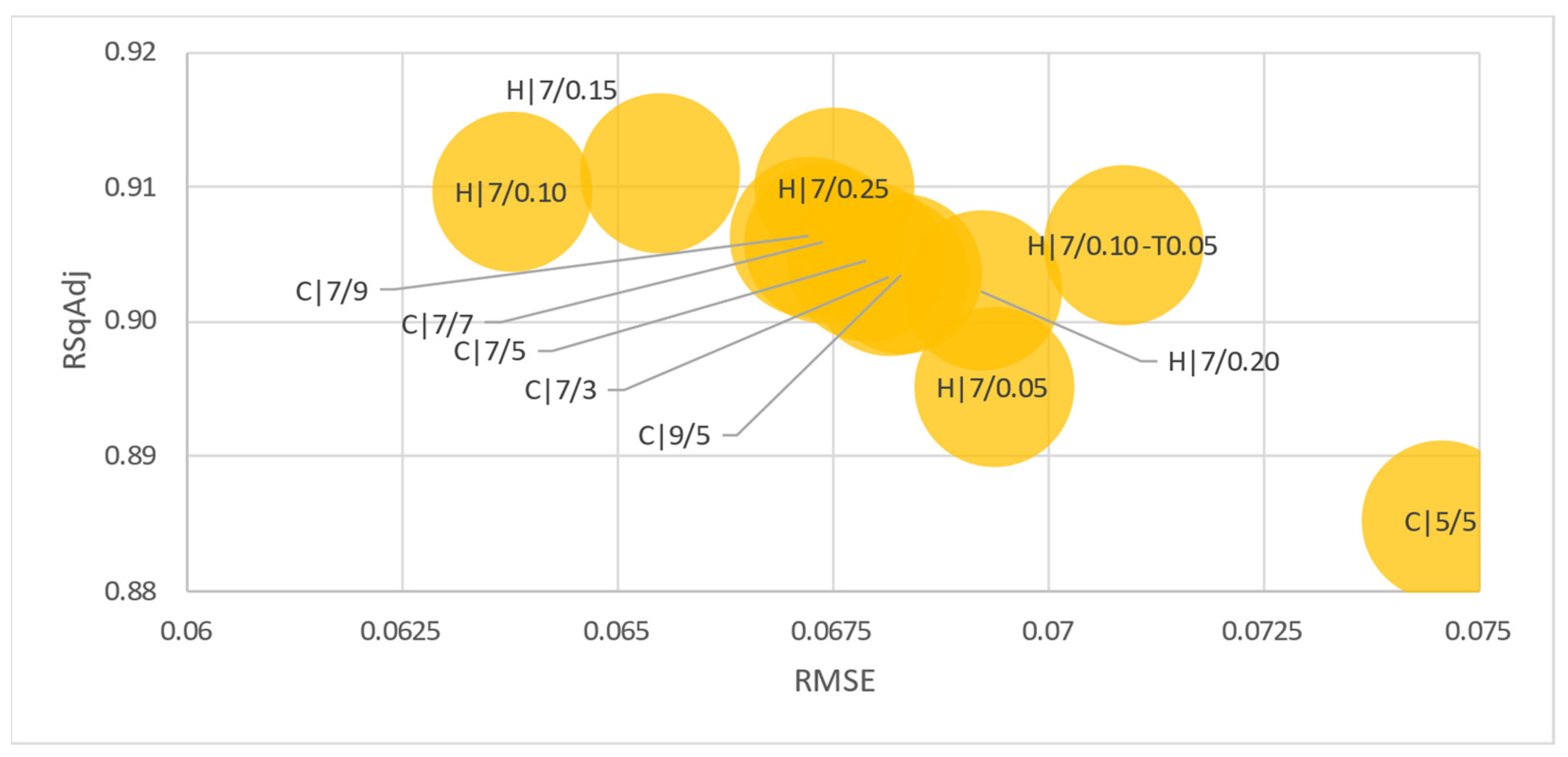
| Model Type | Subtype | Analysis | Minimum RMSE | RSq Adj |
|---|---|---|---|---|
| Ensemble | Boosted Trees | Seven predictors, hold-out 5% (H|7/0.05) | 0.0783 | 0.8664 |
| Bagged Trees | Seven predictors, hold-out 5% (H|7/0.05) | 0.0697 | 0.8940 | |
| Gaussian Process Regression (GPR) | Exponential GPR | Seven predictors, hold-out 10% (H|7/0.10) | 0.0638 | 0.9096 |
| Squared Exponential GPR | Seven predictors, hold-out 10% (H|7/0.10) | 0.0650 | 0.9060 | |
| Matern 5/2 GPR | Seven predictors, hold-out 10% (H|7/0.10) | 0.0648 | 0.9068 | |
| Rational Quadratic GPR | Seven predictors, hold-out 10% (H|7/0.10) | 0.0646 | 0.9074 | |
| Kernel | SVM Kernel | Seven predictors, hold-out 10% (H|7/0.10) | 0.1031 | 0.7639 |
| Least Squares Regression Kernel | Seven predictors, hold-out 10% (H|7/0.10) | 0.1108 | 0.7274 | |
| Linear regression | Linear | Seven predictors, hold-out 5% (H|7/0.05) | 0.0769 | 0.8710 |
| Robust Linear | Seven predictors, hold-out 5% (H|7/0.05) | 0.0772 | 0.8702 | |
| Interactions Linear | Five predictors, cross-over 5-fold (C|5/5) | 0.0839 | 0.8545 | |
| Neural Network | Narrow Neural Network | Seven predictors, hold-out 15% (H|7/0.10) | 0.0716 | 0.8936 |
| Medium Neural Network | Seven predictors, hold-out 10% (H|7/0.10) | 0.0741 | 0.8779 | |
| Wide Neural Network | Five predictors, cross-over 5-fold (C|5/5) | 0.0816 | 0.8626 | |
| Bi-layered Neural Network | Seven predictors, hold-out 10% (H|7/0.10) | 0.0702 | 0.8906 | |
| Tri-layered Neural Network | Seven predictors, hold-out 10% (H|7/0.10) | 0.0715 | 0.8864 | |
| Stepwise Linear Regression | Stepwise Linear | Five predictors, cross-over 5-fold (C|5/5) | 0.0839 | 0.8545 |
| Support Vector Machines (SVM) | Linear SVM | Seven predictors, hold-out 5% (H|7/0.05) | 0.0775 | 0.8690 |
| Quadratic SVM | Seven predictors, hold-out 10% (H|7/0.10) | 0.0662 | 0.9025 | |
| Cubic SVM | Seven predictors, hold-out 10% (H|7/0.10) | 0.0684 | 0.8959 | |
| Fine Gaussian SVM | Three predictors, cross-over 5-fold (C|5/5) | 0.0978 | 0.8028 | |
| Medium Gaussian SVM | Seven predictors, hold-out 10% (H|7/0.10) | 0.0650 | 0.9060 | |
| Coarse Gaussian SVM | Seven predictors, hold-out 10% (H|7/0.10) | 0.0721 | 0.8844 | |
| Tree | Fine Tree | Seven predictors, hold-out 5% (H|7/0.05) | 0.0845 | 0.8444 |
| Medium Tree | Seven predictors, hold-out 5% (H|7/0.05) | 0.0812 | 0.8564 | |
| Coarse Tree | Seven predictors, hold-out 5% (H|7/0.05) | 0.0821 | 0.8530 |
| Tractor Family | Model Type Preset | RMSE | RSqAdj | Observations |
|---|---|---|---|---|
| A|Bb | Optimized Gaussian Process Regression | 0.0546 | 0.9012 | 78 |
| A|Ea | Optimized Gaussian Process Regression | 0.0697 | 0.8157 | 215 |
| A|Gb | Optimized Gaussian Process Regression | 0.0735 | 0.8191 | 224 |
| E|Ea | Exponential GPR | 0.0700 | 0.8334 | 259 |
| E|Ib | Interactions Linear | 0.0780 | 0.3124 | 52 |
| F|Ea | Linear | 0.0764 | 0.7246 | 66 |
| F|Fa | Optimized Gaussian Process Regression | 0.0639 | 0.6549 | 64 |
| F|Fb | Exponential GPR | 0.0628 | 0.8868 | 378 |
| F|Gb | Optimized Gaussian Process Regression | 0.0880 | 0.7505 | 409 |
| F|Ib | Optimized Gaussian Process Regression | 0.0803 | 0.8025 | 244 |
| Tractor Family | Power Linear Regression | Optimized Gaussian Process Regression (GPR) | Observations | ||
|---|---|---|---|---|---|
| RMSE | RSqAdj | RMSE | RSqAdj | ||
| A|Bb | 0.0154 | 0.9804 | 0.0546 | 0.9012 | 80 |
| F|Fb | 0.0182 | 0.9695 | 0.0629 | 0.8863 | 386 |
| F|Fa | 0.0287 | 0.9434 | 0.0639 | 0.6549 | 66 |
| A|Ea | 0.0279 | 0.9657 | 0.0697 | 0.8157 | 216 |
| E|Ea | 0.0796 | 0.9629 | 0.0700 | 0.8333 | 262 |
| A|Gb | 0.0068 | 0.9713 | 0.0735 | 0.8191 | 225 |
| F|Ea | 0.0215 | 0.9522 | 0.0764 | 0.7246 | 70 |
| E|Ib | 0.0173 | 0.9492 | 0.0796 | 0.2832 | 55 |
| F|Ib | 0.0196 | 0.9561 | 0.0803 | 0.8025 | 247 |
| F|Gb | 0.0227 | 0.9505 | 0.0880 | 0.7505 | 410 |
| Author | RMSE | RSqAdj | Observations |
|---|---|---|---|
| Cross, T. L., and Perry, G. M. (1995). | 12.4901 | 0.7573 | 9630 |
| Unterschultz, J., and Mumey, G. (1996). | 11.7518 | 0.4234 | 5417 |
| Cross, T. L., and Perry, G. M. (1996). | 1.0615 | 0.4634 | 9630 |
| Wu, J., and Perry, G. M. (2004). | 6.8064 | 0.7389 | 9630 |
| Fenollosa, M. L., and Guadalajara, N. (2007). | 7.2109 | 0.5272 | 6768 |
| Wilson, P., and Tolley, C. (2004). | 18.2890 | 0.7628 | 9630 |
| Wilson, P. (2010). OLS | 9.9710 | 0.7736 | 9630 |
| Wilson, P. (2010). Box–Cox | 42.7132 | 0.7326 | 9630 |
| ASABE. (2011 (R2020)). | 21.8687 | 0.7435 | 9630 |
| Kay, R., Edwards, W., and Duffy, P. (2020). | 14.2284 | 0.6508 | 8157 |
| Witte, F., Back, H., Sponagel, C., and Bahrs, E. (2022) | 10.6769 | 0.5314 | 8823 |
| Ruiz-Garcia and Sanchez-Guerrero (2022) | 9.3372 | 0.8149 | 10,253 |
Disclaimer/Publisher’s Note: The statements, opinions and data contained in all publications are solely those of the individual author(s) and contributor(s) and not of MDPI and/or the editor(s). MDPI and/or the editor(s) disclaim responsibility for any injury to people or property resulting from any ideas, methods, instructions or products referred to in the content. |
© 2023 by the authors. Licensee MDPI, Basel, Switzerland. This article is an open access article distributed under the terms and conditions of the Creative Commons Attribution (CC BY) license (https://creativecommons.org/licenses/by/4.0/).
Share and Cite
Herranz-Matey, I.; Ruiz-Garcia, L. A New Method and Model for the Estimation of Residual Value of Agricultural Tractors. Agriculture 2023, 13, 409. https://doi.org/10.3390/agriculture13020409
Herranz-Matey I, Ruiz-Garcia L. A New Method and Model for the Estimation of Residual Value of Agricultural Tractors. Agriculture. 2023; 13(2):409. https://doi.org/10.3390/agriculture13020409
Chicago/Turabian StyleHerranz-Matey, Ivan, and Luis Ruiz-Garcia. 2023. "A New Method and Model for the Estimation of Residual Value of Agricultural Tractors" Agriculture 13, no. 2: 409. https://doi.org/10.3390/agriculture13020409
APA StyleHerranz-Matey, I., & Ruiz-Garcia, L. (2023). A New Method and Model for the Estimation of Residual Value of Agricultural Tractors. Agriculture, 13(2), 409. https://doi.org/10.3390/agriculture13020409