Featured Application
This study provides a general methodology for the assessment of the impact of climate change on reliability of structures, combining observations and climate projections, to the aim of giving guidance for the adaptation of climatic load maps in structural Codes.
Abstract
Climatic loads on structures are commonly defined under the assumption of stationary climate conditions; but, as confirmed by recent studies, they can significantly vary because of climate change effects, with relevant impacts not only for the design of new structures but also for the assessment of the existing ones. In this paper, a general methodology to evaluate the influence of climate change on climatic actions is presented, based on the analysis of observed data series and climate projections. Illustrative results in terms of changes in characteristic values of temperature, precipitation, snow, and wind loads are discussed for Italy and Germany, with reference to different climate models and radiative forcing scenarios. In this way, guidance for potential amendments in the current definition of climatic actions in structural codes is provided. Finally, the influence of climate change on the long-term structural reliability is estimated for a specific case study, showing the potential of the proposed methodology.
1. Introduction
The evidence of anthropogenic climate change is widely accepted in the scientific community and many of the observed changes for the period 1950 onwards are unprecedented from over decades to centuries [1].
As it is well known, climate change potentially alters natural processes, causing the modification of precipitation patterns, melting of glaciers, the rise of sea levels, and so on. Whatever the warming scenarios and the level of success of mitigation policies, it is expected that, in the coming decades, climate change effects will become more relevant all around the world, with the impacts of greenhouse gas emissions being time-delayed. For this reason, climate change needs to be considered, taking into account the economic, environmental, and social consequences in many different research fields, inter alia, in structural engineering.
Structural design is often governed by climatic actions, like wind, snow, thermal effects, atmospheric icing, currents, and wave-induced actions. As a consequence, variations of climatic actions due to climate change could significantly affect the design of new structures and infrastructures, as well as the assessment of existing ones, designed in accordance to the provisions of current or past codes [2]. This aspect is crucial since both new and existing structures are supposed to be able to withstand, with the intended degree of reliability, all climatic actions occurring during their whole real life.
It must be highlighted that the real life of structures should not be confused with the notional design working life given in structural codes, as, for example, in Eurocode EN1990 [3], where it is recommended to be at least 50 years for buildings and other common structures and 100 years for monumental buildings and bridges. The notional design working life is intended as a reference time period, during which the structure should meet, without major interventions or repairs, the intended time-dependent performances (e.g., limitation of deterioration or fatigue-induced effects). As it is evident from common experience, constructions, provided that they are properly used and maintained, exhibit real life periods generally significantly greater than their notional design working life, resulting to be extremely sensitive to climate change implications.
As a consequence of the above considerations, constructions designed nowadays will face climatic actions and extreme events, which will be unavoidably be affected by climate change influences. The challenge to estimate these influences is becoming more and more pressing [4].
The definition of climatic actions on structures is currently based on the extreme value analysis applied to past observations of the natural phenomena, under the assumption of stationary climate conditions. Obviously, climate change [1] makes this assumption doubtful, even if a stationary return level and no changes in the frequency of extremes are still often assumed to simplify the problem.
The study of the impact of climate change on climatic actions and consequently on the design of new structures and the assessment of the structural performance of existing structures is then a key aspect in the future evolution of standards. This topic is crucial to achieving an increased resilience of long-life structures and infrastructures to climate change consequences [5], as requested for the second generation of the Eurocodes by the Mandate M/515 of the European Commission to CEN [6].
Characteristic values of climatic actions given in codes are based on observed data series generally covering 40–50 years of measurements; these series are thus not enough extended over time to reflect the effects of the climate change [7] or even to predict future trends. Aiming to account for these aspects, it is, therefore, necessary to rely on climate projections, resulting from appropriate global or regional climate models, which currently are the major source of knowledge about future climate change [8].
In this paper, a general methodology to evaluate the impact of climate change on climatic actions is presented. Starting from the analysis of observed data series and climate projections, provided by different climate models, changes in temperature, precipitation, snow, and wind extremes are discussed for Italy and Germany, considering different climate models and scenarios. In particular, factors of change maps are derived, providing guidance for potential amendments in the current definition of climatic actions in structural codes.
Finally, the influence on the long-term structural reliability of existing structures is assessed, considering the non-stationary nature of climatic actions in the evaluation of failure probability.
2. Climatic Actions on Structures
2.1. Definition of Climatic Loads
In Europe, climatic loads for structural design are defined in the Eurocodes, for snow loads (EN1991-1-3 [9]), wind actions (EN1991-1-4 [10]), and thermal actions (EN1991-1-5 [11]). In the verification of the structural performance, characteristic values of the climatic actions are associated with a given probability of exceedance in a reference period.
As stated in EN1990 [3], characteristic values of climatic actions given in the Eurocodes are associated to a probability of 2% of the time-varying part being exceeded in one year, leading approximately to a return period of 50 years.
Characteristic values of climatic actions and their maps are typically considered country-specific data, to be included in National Annexes to the Eurocodes, as Nationally Determined Parameters (NDP), so that maps for characteristic ground snow loads , basic wind velocity , and maximum and minimum shade air temperature, and , are given in relevant National Annexes to EN1993-1-3 [9], EN1993-1-4 [10], and EN1993-1-5 [11].
Although different procedures for the analysis of extremes are adopted by different countries, as it will be discussed in the following paragraph, the current definition of characteristic values of climatic actions is usually based on the extreme value analysis of past observations of the natural phenomena, under the already mentioned assumption of stationary climate conditions, disregarding potential effects of climate change.
2.2. Classical Extreme Value Theory
The classical extreme value theory provides a rigorous framework for the analysis of climate extremes and their return period. The cornerstone of extreme values theory is the extremal types of theorem [12], providing the convergence of the distribution of maxima to one of the three limiting distributions usually referred as Gumbel or extreme value type I distribution [13,14], Fréchet or extreme value type II distribution [15], and Weibull or extreme value type III distribution [16]. As known, the three extremes values distributions behave differently, but they can be grouped into a single family of three-parameter distributions, the generalized extreme value distribution (GEV) or Fisher–Tippett distribution [17], characterized by the following cumulative distribution function:
defined on the set , where the extreme value parameters location , scale , and shape satisfy the inequalities: ; ; . The type II (Fréchet) and type III (Weibull) classes of extreme value distributions correspond respectively to the cases and , and the subset of the GEV family with can be interpreted as the limit of Equation (1) where , corresponding to the type I (Gumbel) with cumulative distribution function
where the location parameter specifies the center of the distribution and the scale parameter σ determines the size of deviations around the location parameter.
Extreme value type I distribution is often assumed as the limiting distribution for maxima in the definition of characteristic values of climatic actions [18], which can be determined by means of the formula
where is the probability of exceedance in one year, which, according to EN1990 [3], is taken as .
2.3. Non-Stationary Extremes
As mentioned above, in a changing climate, the assumption of stationarity is becoming debatable. The frequency of extreme events is continuously evolving and changes are likely to continue in the future. Therefore, the growing interest in this field is leading to the definition of non-stationary extreme value models, where time dependence is taken into account defining trends of the extreme value distribution parameters. These trends are usually modeled in climatology, assuming the existence of a functional relationship between the distribution parameters, and , and time. Although different models may be defined, simple linear or log-linear models are normally used [19,20]; moreover, most applications consider non-stationarity only for the location parameter, assuming the scale parameter is nearly constant [21].
Nevertheless, considerable uncertainties remain in the definition of the trend model; in fact, since, as already remarked, observed data series for current definition of climatic actions generally cover up to 50-year measurements, the simple analysis of maxima in a given time period, commonly annual maxima, is often not appropriate to identify univocal trends.
Finally, as shown in [22], extremes in a changing climate are more sensitive to changes in the variability associated to the scale parameter, than to changes of the mean value, to which the location parameter is associated. Consequently, assuming a constant scale parameter seems to be inappropriate, such a hypothesis completely neglects this aspect.
In the present study, the analyses are then oriented toward a sound definition of non-stationary extremes, also suitable for structural design. The innovation of the proposed approach is that trends are directly assessed on characteristic values, dividing the entire population of maxima, obtained from the analysis of long-term climate projections in appropriate time windows.
3. Structural Reliability under Non-Stationary Loads
As recalled above, a structure shall be designed and executed in such a way that it will sustain all actions and influences likely to occur during its intended life with an appropriate degree of reliability and in an economical way.
In the Eurocodes, the adoption of characteristic values of actions, in conjunction with the use of the partial factor method in limit state verifications, should lead to the achievement of a reference reliability level, corresponding to a reliability index for a 50-year reference period [3] for a structure with “normal” consequences of failure.
In order to define the probability of failure and then the reliability index , it is assumed that structural behavior is described by a set of random variables describing actions, mechanical properties, geometrical data, and model uncertainties. A limit state function is then defined as the safety margin , where is the structural resistance and the load effect.
Considering that climate change, even if it could potentially act on resistances, mainly affects the actions on the structure [23], this paper focuses on the influence of non-stationary loads on long-term structural reliability, presenting a methodology to evaluate the climate change impact on atmospheric actions.
In previous studies [23,24], time-dependent reliability in the presence of non-stationary loads has been studied considering how the probability of failure varies as a function of the mean value of the load intensity and the load occurrence rate. As illustrated in the following, the present study aims to widen the current horizon of this research field, evaluating time-dependent reliability as a function of changes, not only of the mean values of the environmental loads but also of their variances.
4. Climate Projections for Impact Studies
Nowadays, climate models are the major source of information about future climate. They are process-based dynamical models [25] based on various assumptions, which operate across the entire globe or in a limited region of the world, simulating the physics and chemistry of the atmosphere and oceans to obtain projections of temperature and other meteorological variables. Indeed, they can be run in different modes either considering observed changes in atmospheric composition to reproduce historical climate or according to different scenarios of potential and plausible changes of forcing agents to simulate future climate. In most cases, these scenarios refer to changes in the emission of greenhouse gasses [26], which, manifestly, depend on economic and social development, as well as on political choices.
One of the most relevant parameters in the climate model is the resolution; that is, the dimension of the single cell of the geographical grid used for the simulation. Obviously, finer grids provide more accurate results requiring, in turn, higher processing time.
In this paper, high-resolution regional climate models, based on a 12.5 km resolution (EUR-11) grid, developed within the EURO-CORDEX initiative [27,28], are analyzed.
These regional simulations are obtained by downscaling the new Coupled Model Intercomparison Project (CMPI5) for global climate predictions [29], where future projections are run according to a new set of scenarios, containing emission, concentration, and land-use trajectories, commonly referred to as Representative Concentration Pathways (RCPs) and exhaustively described in [30].
In this study, the RCP4.5 and the RCP8.5 emissions scenarios have been considered for the investigated climate models: RCP4.5 is a midrange mitigation emissions scenario, and RCP8.5 is the highest emission scenario.
Due to the huge processing time needed to provide predictions until 2100, usually each climate model is run once; thus, different climate models are often combined aiming to improve the soundness of the results. A frequently used combination is the so-called multi-model ensemble.
The rationale of multi-model ensemble is that each climate model can be considered as an independent and more or less credible realization of the future climate: if all the models provide credible outputs, they are just combined; if, on the contrary, some models are judged more reliable than the others, for example, considering their ability to reproduce past climate, suitable weights are introduced to differentiate the contribution of single models in the ensemble.
Dealing with multi-model ensemble, a detailed review of different approaches to combine climate models’ output is discussed in [31].
In the present study, unweighted models have been used for the evaluation of changes in environmental parameters. This approach is usually called the Ensemble Mean [32].
5. Methodology to Evaluate the Impact of Climate Change
5.1. Analysis of Climate Projections
For the purpose of this study, daily climate projections of the investigated climate variables—maximum and minimum shade air temperatures, precipitation, maximum wind velocity—for the investigated regions, in the control period 1951–2005 and in the future period 2006–2100, have been preliminarily extracted from the different climate models.
Subsequently, a series of annual maxima have been derived for forty-year long time windows, shifted by ten years of each other: 1951–1990, 1961–2000, …, 2061–2100.
Finally, extreme value analysis has been carried out for each time window, according to the block maxima approach [12]. In the elaboration, an extreme value type I distribution (Equation (2)) has been assumed and the characteristic values of the climatic action, , have been evaluated applying Equation (3), for the -th time window.
In this way, a series of eleven values for have been obtained for each investigated climate model, describing the current and future values of relevant climatic variables.
5.2. Estimation of Factors of Change (FC)
Since values of climatic variables predicted by climate models are more reliable if looked at in relative terms rather than in absolute sense, climate models are particularly effective when used to identify alterations of the statistical properties of climate variables awaited for the future. These alterations between statistics of the climatic variables can be expressed by means of the so-called change factors [33] or factors of change (FC); the latter [34] is the definition adopted here.
The factors of change are concise representations of the changes of characteristic values of the variable between the first time window, , and the n-th one .
Depending on the climatic variable under consideration, factors of change can be defined in terms of differences or in terms of ratios. Factors of change in terms of differences, the so-called delta changes, are typically defined for temperatures as:
Factors of changes in terms of ratios can be defined for precipitations, snow loads, and wind actions as:
Assuming that the first time window corresponds to the observation period used for the definition of the current design loads, the future characteristic values of a given climate variable can be obtained applying the factors of change to its characteristic value, obtained from the real measurements, . In this way, the future characteristic values are given by:
for temperature, and:
for precipitations, snow loads, and wind actions.
In Equations (6) and (7), are the factors of change provided by the appropriate combination of the climate models considered in the multi-model ensemble.
5.3. Evaluation of New Design Loads
The factors of change for the characteristic values of the considered climatic action provide sound guidance for potential amendments of the existing structural codes. Considering that, as discussed before, the real life of a new structure could be significantly greater than its notional design working life, the variations of characteristic values of climatic actions over time can be taken into account in the design of new structures by means of a suitable envelope of the characteristic values obtained for each time window, so that:
where is the number of time windows taken into account.
As is usually the case in structural design, it is assumed that the characteristic value of combined effects of different climatic actions occurs when one of them attains its characteristic value, even if this is not always true. Anyhow, provided that mutual correlations between the actions are properly accounted for, the proposed approach could be extended to the evaluation of factors of changes affecting combinations of correlated climate variables. As a first approximation, a combination of factors could be assumed to remain constant, but, duly comparing the evolution over time of the characteristic values of each climatic action and the corresponding evolution of the characteristic value of the combined ones, it would be possible, through a trial and error process, to evaluate factors of change for combination factors as well. This is one of the objectives of future researches.
6. Application and Results
6.1. Framework of the Study
In the present study available data from the EURO-CORDEX initiative [26,27] have been considered for daily climate projections of maximum and minimum temperature, , , precipitation, , and daily maximum wind speed, . In more detail, they have been examined with data provided by the Danish Meteorological Institute (DMI), the CLM Community (CLMcom), the Royal Netherlands Meteorological Institute (KNMI), the Max Planck Institute (MPI-CSC), the Laboratoire des Sciences du Climat et de l’Environnement—Institute Pierre Simon Laplace (IPSL-INERIS), the and Centre National de Recherches Météorologiques de Météo France (CNRM).
It must be highlighted that each climate projection needs a sort of calibration, which is usually done reproducing past observations in a suitably long period, generally at least 50 years, representing the so-called “control period”. This calibration process, usually called “Historical Experiment”, is carried out aiming to fit data predicted by the considered climate model in the control period with measured ones, in order to assess its capability to correctly reproduce future climate. In the EURO-CORDEX framework, the projections were calibrated assuming “control period” for the “historical experiment” in the period 1951–2005.
In the calibration, the “run” of climate model, being guided by real changes in atmospheric composition in the period 1951–2005, was forced to fit observations. Once calibrated, the climate model was used to predict the “future” outcomes in the period 2006–2100 in several emission scenarios [28,29].
Starting from the model specifications summarized in Table 1 and considering the medium emission scenario (RCP4.5 experiment) and the highest emission scenario (RCP8.5 experiment), the present study focuses on the elaboration of factors of change maps, derived comparing the future predictions provided by several climate models with the corresponding results of the historical experiment.

Table 1.
Overview of the main characteristics of analyzed climate projections.
The outcomes of the analysis, in terms of factors of change maps for precipitation, ground snow load, basic wind velocity, and maximum and minimum air-shade temperature, are presented in the following paragraphs for Italy and Germany.
6.2. Factors of Change Maps for Precipitation
The outcomes of many recent climate studies generally call for an increase in precipitation extremes due to warming climate [35], confirming the observational evidence of heavy rainfall intensifications in several regions all around the world in the last six decades [36,37].
The observations support the classical Clausius–Clapeyron thermodynamic law, which states that warmer air has a higher water vapor holding capacity [38]. As stated by this law, the moisture content of the atmosphere increases with a scaling rate of about , being in Kelvin.
Even if precipitation is not directly considered in the Eurocodes, changes in the frequency and intensity of precipitation extremes may have significant adverse implications on the hydrologic design of water infrastructures, since it can cause an increase of risk of flooding events as well as a reduction of service life of bridges, associated with higher scouring rate of bridge foundations.
Following the methodology previously described, factors of change for characteristic values (2% probability of exceedance on an annual basis) , have been evaluated for Italy and Germany, in terms of ratios, according to Equation (5).
The resulting factors of change maps are presented in Figure 1 and Figure 2 considering three 40-year long time windows: 2011–2050, 2031–2070, and 2051–2090.
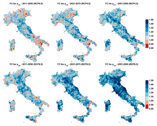
Figure 1.
Precipitation changes in Italy referring to 1951–1990. RCP4.5 (1st row). RCP8.5 (2nd row).
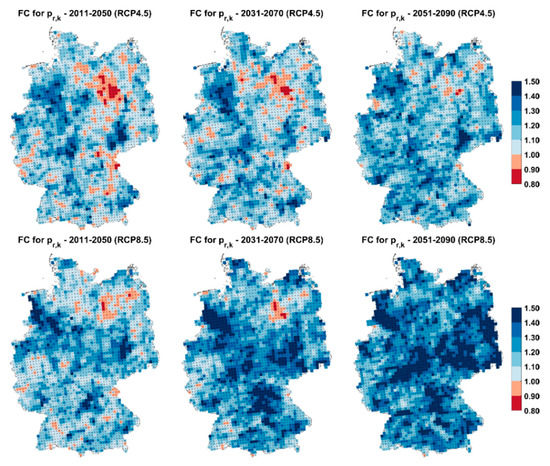
Figure 2.
Precipitation changes in Germany referring 1951–1990. RCP4.5 (1st row). RCP8.5 (2nd row).
In the figures, maps in the first row refer to medium RCP scenario (RCP4.5), and maps in the second row refer to the highest RCP scenario (RCP8.5).
The maps confirm that significant changes can occur. Strong increases are awaited for in large parts of the Italian and German territories, especially when the highest emission scenario RCP8.5 is taken into account, thus further validating the conclusions of previous studies about the influence of global warming on precipitation extremes [39,40].
6.3. Factors of Change Maps for Ground Snow Loads
One of the conventional remarks about global warming is that a reduction of snow is expected as a consequence of the increase of mean temperature, but this is not always true, at least at a local scale. In fact, although a decrease in mean snowfall is expected in most regions due to the decrease of snowfall frequency, a contrasting response may be experienced in other regions for snowfall extremes [41]. The snowfall rate can increase as a result of the intensification of precipitation rate, combined with the decrease of snowfall fraction when the former aspect prevails in the future trends [41,42].
To evaluate the impact of climate change on snow load and on structures, a general methodology to derive snow loads from daily outputs of climate models (maximum and minimum temperature and precipitation) has been developed by the authors, as illustrated and discussed in detail in [2]. In the present research, the proposed algorithm has been suitably implemented in order to obtain, on the basis of daily climate projections available for the two different RCPs scenarios recalled above, yearly maxima series of the ground snow loads. These series have been subsequently analyzed to derive a factor of changes for characteristic values of snow load, , in terms of ratio, according to Equation (5).
The resulting factors of change maps for the Italian part of the European Mediterranean climatic region defined in [9] are shown in Figure 3 for the three time windows: 1991–2030, 2011–2050, and 2031–2070.
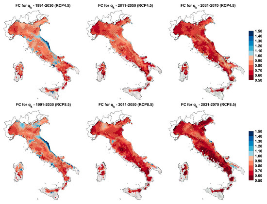
Figure 3.
Characteristic ground snow load factors of change in Italy referring to 1951–1990. RCP4.5 (1st row). RCP8.5 (2nd row).
The outcomes show a general decreasing trend for the investigated region, even if trends can be different depending on the considered area on the considered time window and on the reference emission scenario. In the near-term future (1991–2030), a constant or increasing trend (FC > 0.95) may be expected in the northern and eastern Italian regions [7]; however, a decrease is projected in a long-term future (2031–2070), substantially confirming the general remark recalled at the beginning of this subsection.
The factors of change maps shown in Figure 4 are referred to as the German part of the European central east climatic region defined in [9]. Similar conclusions to those expressed for the Italian territory can be drawn for Germany.
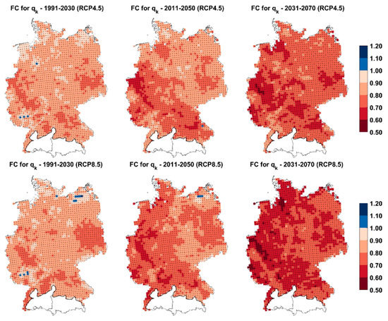
Figure 4.
Characteristic ground snow load factors of change in Germany referring to 1951–1990. RCP4.5 (1st row). RCP8.5 (2nd row).
6.4. Factors of Change Maps for Wind Loads
As highlighted by recent investigations, specifically devoted to assessing the impact of climate change effects on wind energy production [43], climate change may also alter the geographical distribution and intensity of near-surface winds.
Influence of climate change in terms of wind speed and wind energy potentials have been particularly studied in [44], where, on the basis of an ensemble of EURO-CORDEX climate projections, a decrease of wind energy output for most of Europe has been assessed in the coming decades, even if updated climate change trends in central Europe seem generally less evident than previously predicted.
Near-surface wind velocities provided by the multi-model ensemble described in Section 6.1 have been analyzed, focusing the attention on extremes, in order to identify factors of change for characteristic wind speed, , in terms of ratio, according to Equation (5), for medium and highest emission scenarios, RCP4.5 and RCP8.5, respectively.
The results in terms of factors of change maps obtained for Italy and Germany are illustrated in Figure 5 and Figure 6, respectively, considering again the three forty-year long time windows 2011–2050, 2031–2070, and 2051–2090.
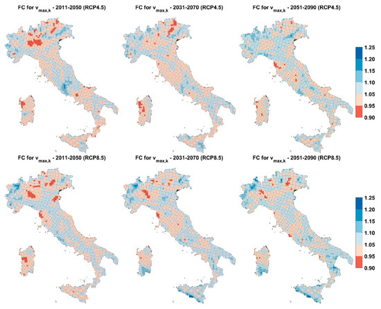
Figure 5.
Characteristic wind speed changes in Italy referring to 1951–1990. RCP4.5 (1st row). RCP8.5 (2nd row).
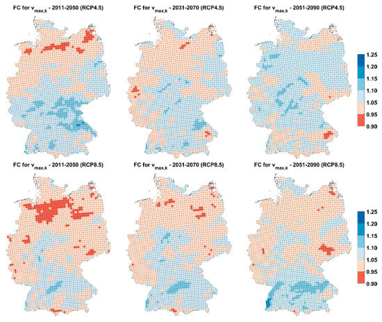
Figure 6.
Characteristic wind speed changes in Germany referring to 1951–1990. RCP4.5 (1st row). RCP8.5 (2nd row).
The outcomes show that in the two investigated regions, changes in the characteristic wind speed are not particularly significant. In fact, factors of change fall within the interval 0.95–1.05 in most of the regions and their values are nearly independent on the emission scenario.
For example, considering characteristic wind speed in the period 2031–2070:
- In the RCP4.5 scenario:
- ○
- Factors of change in the interval 0.95–1.05 cover approximately 96% of Germany and 94% of Italy;
- ○
- Factors of change greater than 1.05 are expected only at approximately 3.7% of the Italian land and 2.6% of the German land;
- In the RCP8.5 scenario:
- ○
- Factors of change in the interval 0.95–1.05 cover approximately 95% of Germany and 91% of Italy;
- ○
- The extension of the zones affected by factors of change higher than 1.05 increases to approximately 6.9% of the Italian territory and 3.1% of the German one.
Similar effects are expected in the long-term future, i.e., in the period 2051–2090.
6.5. Factors of Change Maps for Thermal Actions
Thermal actions on buildings, bridges, and other structures in Europe are given in EN1991-1-5 [11]. Temperature variation within an individual structural element is split into four elementary components (uniform temperature, linear horizontal differential, linear vertical differential, and non-linear differential), as illustrated in Figure 4.1 of Eurocode EN1991-1-5 [10]. These components are functions of the already defined characteristic values of maximum and minimum shade air temperatures, and , at the construction site, given in the National Annex.
Using the proposed approach, the factors of change for and have been derived for the RCP4.5 and the RCP8.5 emission scenarios in terms of difference, according to Equation (4).
Considering Italy and the time windows 2011–2050, 2031–2070, and 2051–2090, the factor of change maps for and obtained are presented in Figure 7 and Figure 8, respectively.
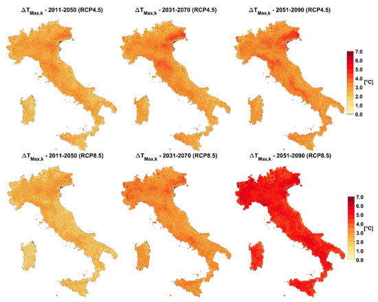
Figure 7.
Characteristic maximum temperature changes in Italy referring to 1951–1990. RCP4.5 (1st row). RCP8.5 (2nd row).
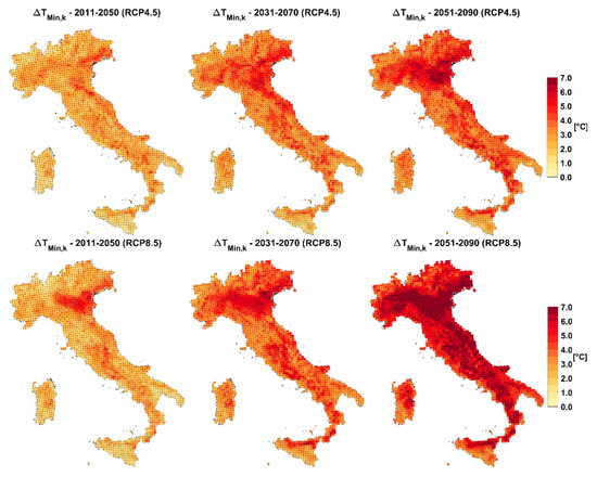
Figure 8.
Characteristic minimum temperature changes in Italy with respect to 1951–1990. RCP4.5 (1st row). RCP8.5 (2nd row).
The maps show a general increasing trend in line with the expectations about global warming, but variations of characteristic values are much more significant than variations of mean temperature values.
Actually, in Italy, in the long-term future (2051–2090), increases up to 5.5 °C may be expected for maximum shade air temperature and up to 6 °C for minimum shade air temperature.
In Figure 9 and Figure 10, they are illustrated as the maps elaborated for Germany, which lead to similar conclusions to those already reported for Italy.
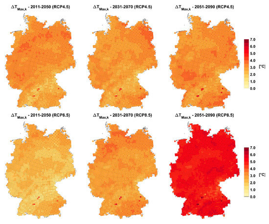
Figure 9.
Characteristic maximum temperature changes in Germany referring to 1951–1990. RCP4.5 (1st row). RCP8.5 (2nd row).
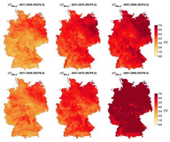
Figure 10.
Characteristic minimum temperature changes in Germany referring to 1951–1990. RCP4.5 (1st row). RCP8.5 (2nd row).
In this case, the percentage of the region affected by the highest variations () is much more evident for minimum temperature (54.9% and 96.5% according to the RCP4.5 and RCP8.5, respectively).
7. Impact of Climate Change on Structural Reliability
The dependency of structural reliability on the non-stationary nature of climatic loads and its evolution over time is a modern research topic inside the structural engineering community [45,46].
A methodology to estimate time-dependent reliability of aging structures accounting for non-stationarity of structural loads and for the variability of structural deterioration phenomena is, for example, proposed in [24]. This method assumes the deterioration of structural resistance as a function of time by means of the following expression:
where is the initial resistance and is a suitable degradation function.
The non-stationarity of the structural loads is taken into account assuming both the mean load intensity and the mean occurrence rate as functions of time.
The hazard function or conditional failure rate at time , , i.e., the probability of structural failure during interval given that the structure survives over , is defined as in [24]:
where is the cumulative distribution function (CDF) of the load intensity, often described by an extreme value type I distribution.
The hazard function can be also related to the time-dependent structural reliability as reported in [47]. Indeed, it can be written as the ratio between the probability density function of the time to failure, i.e., the derivative of , and the structural reliability function , arriving to the following expression:
Finally, combining Equations (10) and (11), the time-dependent structural reliability becomes:
and the probability of failure trivially results:
In this study, the time-dependent structural reliability is evaluated introducing in Equation (12) the variation over time of obtained following the above-described approaches.
Among the outcomes of the analysis, particularly relevant are the factors of changes pertaining to the th time window, and affecting the mean load intensity, and the standard deviation, , of the annual maxima of the climatic action under examination.
Assuming an extreme value type I distribution, its location and its scale parameter, and are given by:
where is the starting time of the considered time window:
being the time interval separating two consecutive time windows.
Consequently, Equation (12) can be rewritten as:
Since, in the present case, the distance between adjacent time windows, each one forty-year long, is ten years, factors of changes and regarding the CDF of the action intensity are evaluated every ten years. The reliability at the time is then computed in the following way:
where is expressed in years.
The following example illustrates the application of the method to assess the variation of the snow load expected at a specific location in Italy. To develop that example, the design criteria illustrated in [24] and the reliability targets given in the Eurocode EN1990 have been adopted.
The investigated Italian cell is located in the Emilia Romagna region. The cell, sized 12.5 km, is numbered 1230. As shown in Figure 11, the center of the cell is close to the small town of Borghi, approximately 14 km away as the crow flies from the Adriatic coast.
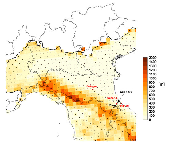
Figure 11.
Location of the Italian cell no. 1230 (Emilia Romagna region).
In the example, the factors of change of mean value, , standard deviation, , and characteristic value, , of ground snow load in the cell have been estimated as a function of time according to Section 6.
The results are shown in Figure 12, where the red line, the blue line, and the green line illustrate the evolution over time of the factors of change for mean value, , standard deviation, , and characteristic value, , respectively, referring to the RCP8.5 scenario.
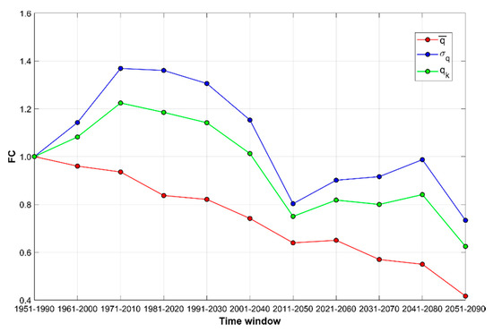
Figure 12.
FC-time curves for , , and of ground snow load in cell 1230. RCP8.5 scenario.
Adopting the same probabilistic models of resistance and load intensity used in [24] and reported in Table 2, the variation of the probability of failure over time has been then evaluated, considering the resistance a deterministic linear degradation function:
where is the degradation rate parameter.
Table 2.
Statistical description of structural resistance and loads.
The target reliability index for a reference period of 50 years has been set, as indicated in EN1990 [3], , so that the actual reliability index of the structure should satisfy:
where is the design working life of the structure itself.
In the example, considering a design working life of the construction , Equation (20) is satisfied when the total degradation does not exceed , which implies and , in case of stationary load.
As suggested in [24], the hypotheses are that, during the investigated period, no interventions are implemented to restore the initial resistance of the structure, and that the main source of randomness is the variable action.
Following the classical load and resistance factor design method (LRFD) [48], the permanent load and the variable load (snow load in this case), modeled as in Table 2, are combined as in [24] according to the load combination given in ACI standard 318-89 [49], . The resulting total design load is set equal to the reduced design strength, , leading to the following design Equation:
where, for simplicity, is set equal to , as it was done in [24].
The results are shown in Figure 13, in the form of diagram (a) and diagram (b), where:
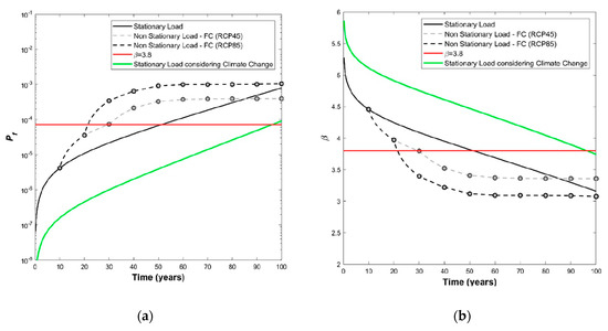
Figure 13.
Variation over time of: (a) probability of failure ; (b) reliability index .
- Results in case of stationary load hypothesis are shown with solid black lines;
- Dashed gray lines refer to non-stationary load and medium emission scenario (RCP4.5);
- Dashed black lines refer to non-stationary load and highest emission scenario (RCP8.5).
In the diagrams, the green lines illustrate the variations over time in case the design is based on the maximum characteristic load calculated taking into account the effects of climate change, according to the methodology proposed in Section 6.3. In the example, as evident in Figure 12, this characteristic load is higher than that corresponding to the stationary assumption being affected by a factor of change around 1.23 (time window 1971–2010).
Inspecting the diagrams, it clearly results that:
- Apparently, in case of stationary load assumption, the structure satisfies the minimum assumed reliability requirements for its design working life, 50 years, and, in absence of interventions, in 100 years its reliability index decreases till to ;
- On the contrary, adopting the reliability index is increased, so that in the example the structural reliability would remain adequate even for 100 years;
- In the RCP4.5 scenario, the structure satisfies minimum reliability requirements for 30 years; its reliability index decreases to at the end of the design working life;
- In the RCP8.5 scenario, the structure satisfies minimum reliability requirements for 20 years; its reliability index decreases to at the end of the design working life;
- Therefore, the implementation of suitable adaptation measures is necessary to guarantee that the expected reliability does not reduce too much;
- Moreover, since effects of climate change in a long-term future claim for a reduction of snow loads, the reliability index after 100 years results in the RCP4.5 scenario and in the RCP8.5, thus compensating in some way the degradation of the resistance; but, of course, it is not always the case. Evidently, different trends for climatic loads, such as constant increases, further reduce the reliability in the long-term future.
Obviously, the conclusions drawn here about the variation of the reliability index are indicative and clearly depend upon the design criteria and on the reliability target values assumed in the analysis and cannot be generalized.
In any case, it must be underlined that, to better cover model uncertainties as well as to set a minimum value for loads on the roof, often characteristic snow loads given in codes overestimate the loads resulting from the statistical elaborations of data, so introducing some additional intentional safety margin as discussed, for example, in [50] is required.
8. Conclusions
A general methodology to evaluate the climate change effects on relevant climatic actions and the associated impact on structural reliability is presented based on the analysis of observed data series and climate models’ projections.
The topic is very relevant since, in the current structural codes, representative values of climatic actions are usually based on the analysis of past observations under the hypothesis of stationary future climate, disregarding potential effects of climate change.
Changes in extremes of the underlying climatic variables, like precipitations, snow loads on the ground, wind velocity, and maximum and minimum shade air temperature, are estimated analyzing high-resolution climate projections provided by different climate models in suitably spaced different time windows. Subsequently, to take into account future trends and to quantify the consequences of future climate change on structural reliability, factors of change are derived, aiming to adapt values of climatic actions provided by structural codes.
The outcomes of the procedure are presented in factors of change maps, obtained for Italy and Germany, considering forty-year time windows in two alternative cases, corresponding to the medium (RCP4.5) and to the highest (RCP8.5) greenhouse gas emission scenarios.
The factor of change maps, which are given for the four considered climatic variables (precipitation, snow load on ground, wind velocity, and maximum and minimum air shade temperature), provide guidance for potential amendments and improvements of climatic actions in structural codes, especially in the Eurocodes.
Finally, the potential influence of climate change on structural reliability is tackled, in a simple but explanatory case study, focusing on the variability of snow loads in time. Duly taking into account the non-stationary nature of climatic actions linked to climate change, the time-dependent structural reliability is evaluated based on the predicted changes in mean load intensity and standard deviation of annual maxima of snow loads.
The results indicate that effects of climate change could cause a reduction over time of the structural reliability, more significant than that expected in stationary climate conditions, due to resistance’s degradation effects. Consequently, the required target reliability is not reached for the design working life of the construction.
Therefore, to maintain the required reliability level, climatic actions would need some adaptation to take into account the effect of climate change.
It must be remarked that a wider field of application and improvements can be envisaged for the proposed methodology, for example:
- On the one hand, as previously mentioned, it could be applied also to evaluate factor of changes of combination factors as well as factors of change for combinations of correlated variables;
- On the other hand, it could be sensibly improved by the implementation of suitably updated weather generators [34,51] and stochastic downscaling techniques [52,53].
Investigation of these promising subjects will be the objective of further studies.
Author Contributions
Conceptualization, P.C., P.F., and F.L.; methodology, P.C., P.F., and F.L.; software, P.C., P.F., and F.L.; validation, P.C., P.F., and F.L.; writing—original draft preparation, P.C., P.F., and F.L.; writing—review and editing, P.C., P.F., and F.L.; resources, P.C.
Funding
This research received no external funding.
Acknowledgments
We acknowledge: the World Climate Research Programme’s Working Group on Regional Climate, and the Working Group on Coupled Modelling, former coordinating body of CORDEX and responsible panel for CMIP5; the climate modelling groups (listed in Table 1 of this paper) for producing and making available their model output; the Earth System Grid Federation infrastructure an international effort led by the U.S. Department of Energy’s Program for Climate Model Diagnosis and Intercomparison; the European Network for Earth System Modelling and other partners in the Global Organization for Earth System Science Portals (GO-ESSP); our colleagues of the units: Safety and Security of Buildings and Disaster Risk Management of European Commission, Joint Research Centre, Ispra (IT).
Conflicts of Interest
The authors declare no conflicts of interest.
References
- Stocker, T.F.; Qin, D.; Plattner, G.-K.; Tignor, M.; Allen, S.K.; Boschung, J.; Nauels, A.; Xia, Y.; Bex, V.; Midgley, P.M. Climate Change 2013: The Physical Science Basis. Contribution of Working Group I to the Fifth Assessment Report of the Intergovernmental Panel on Climate Change; Cambridge University Press: Cambridge, UK; New York, NY, USA, 2013. [Google Scholar]
- Croce, P.; Formichi, P.; Landi, F.; Marsili, F. Climate change: Impact on snow loads on structures. Cold Reg. Sci. Technol. 2018, 150, 35–50. [Google Scholar] [CrossRef]
- EN 1990. Eurocode—Basis of Structural Design; CEN: Brussels, BE, USA, 2002. [Google Scholar]
- Madsen, H.O. Managing structural safety and reliability in adaptation to climate change. In Safety, Reliability, Risk and Life-Cycle Performance of Structures and Infrastructure; Deodatis, E.F., Ed.; Taylor & Francis Group: London, UK, 2013; pp. 81–88. ISBN 978-1-315-88488-2. [Google Scholar]
- European Commission. M/515 EN—Mandate for Amending Existing Eurocodes and Extending the Scope of Structural Eurocodes; European Commission: Brussels, Belgium, 2012. [Google Scholar]
- CEN/TC250. Response to Mandate M/515—Towards a Second-Generation of Eurocodes; CEN-TC250—N 993: Brussels, Belgium, 2013. [Google Scholar]
- Croce, P.; Formichi, P.; Landi, F.; Mercogliano, P.; Bucchignani, E.; Dosio, A.; Dimova, S. The snow load in Europe and the climate change. Clim. Risk Manag. 2018, 20, 138–154. [Google Scholar] [CrossRef]
- Maraun, D. Bias Correcting Climate Change Simulations—A Critical Review. Curr. Clim. Chang. Rep. 2016, 2, 211–220. [Google Scholar] [CrossRef]
- EN 1991-1-3. Eurocode 1: Actions on Structures—Part 1–3: General Actions—Snow Loads; CEN: Brussels, Belgium, 2003. [Google Scholar]
- EN 1991-1-4. Eurocode 1: Actions on Structures—Part 1–4: General Actions—Wind Actions; CEN: Brussels, Belgium, 2005. [Google Scholar]
- EN 1991-1-5. Eurocode 1: Actions on Structures—Part 1–5: General Actions—Thermal Actions; CEN: Brussels, BE, USA, 2003. [Google Scholar]
- Coles, S. An Introduction to Statistical Modelling of Extreme Values; Springer-Verlag: London, UK, 2001. [Google Scholar]
- Gumbel, E.J. Les valeurs extrêmes des distributions statistiques. Annales de L’institut Henri Poincar 1935, 5, 115–158. [Google Scholar]
- Gumbel, E.J. Statistics of Extreme; Columbia University Press: New York, NY, USA, 1958. [Google Scholar]
- Fréchet, M. Sur la loi de probabilité de l’écart maximum. Ann. Soc. Polon. Math. 1927, 6, 93–116. [Google Scholar]
- Weibull, W. A statistical distribution function of wide applicability. J. Appl. Mech.-Trans. ASME 1951, 18, 293–297. [Google Scholar]
- Fisher, R.A.; Tippett, L.H.C. Limiting Forms of the Frequency Distribution of the Largest and Smallest Member of a Sample. Math. Proc. Camb. Philos. Soc. 1928, 24, 180–190. [Google Scholar] [CrossRef]
- Formichi, P.; Danciu, L.; Akkar, S.; Kale, O.; Malakatas, N.; Croce, P.; Nikolov, D.; Gocheva, A.; Luechinger, P.; Fardis, M.; et al. Eurocodes: Background and applications. Elaboration of maps for climatic and seismic actions for structural design with the Eurocodes. JRC Sci. Policy Rep. 2016. [Google Scholar] [CrossRef]
- Cheng, L.; AghaKouchak, A.; Gilleland, E.; Katz, R.W. Non-stationary extreme value analysis in a changing climate. Clim. Chang. 2014, 127, 353–369. [Google Scholar] [CrossRef]
- Begueria, S.; Angulo-Martínez, M.; Vicente-Serrano, S.M.; López-Moreno, J.I.; El-Kenawyet, A. Assessing trends in extreme precipitation events intensity and magnitude using non-stationary peaks-over-threshold analysis: A case study in northeast Spain from 1930 to 2006. Int. J. Climatol. 2011, 31, 2102–2114. [Google Scholar] [CrossRef]
- Renard, B.; Sun, X.; Lang, M. Bayesian methods for non-stationary extreme value analysis. In Extremes in a Changing Climate; Agha Kouchak, A., Easterling, D., Hsu, K., Schubert, S., Sorooshian, S., Eds.; Springer: Dordrecht, The Netherlands, 2013. [Google Scholar] [CrossRef]
- Katz, R.W.; Brown, B.G. Extreme events in a changing climate: Variability is more important than averages. Clim. Chang. 1992, 21, 289–302. [Google Scholar] [CrossRef]
- Saini, A.; Tien, I. Impacts of Climate Change on the Assessment of Long-Term Structural Reliability. J. Risk Uncertain. Eng. Syst. Part A Civ. Eng. 2017, 3. [Google Scholar] [CrossRef]
- Li, Q.; Wang, C.; Ellingwood, B. Time-dependent reliability of aging structures in the presence of non-stationary loads and degradation. Struct. Saf. 2015, 52, 132–141. [Google Scholar] [CrossRef]
- Muller, P.; von Storch, H. Computer Modeling in Atmospheric and Oceanic Sciences; Springer: Berlin/Heidelberg, Germany, 2004. [Google Scholar]
- von Storch, H. Models of Global and Regional Climate. In Encyclopedia of Hydrological Sciences; Anderson, M.G., Ed.; John Wiley & Sons: New York, NY, USA, 2006. [Google Scholar]
- Jacob, D.; Petersen, J.; Eggert, B.; Alias, A.; Christensen, O.B.; Bouwer, L.M.; Braun, A.; Colette, A.; Déqué, M.; Georgievski, G.; et al. EURO-CORDEX: New high-resolution climate change projections for European impact research. Reg. Environ. Chang. 2014, 14, 563–578. [Google Scholar] [CrossRef]
- Kotlarski, S.; Keuler, K.; Christensen, O.B.; Colette, A.; Déqué, M.; Gobiet, A.; Goergen, K.; Jacob, D.; Lüthi, D.; van Meijgaard, E.; et al. Regional Climate Modelling on European Scale: A joint standard evaluation of the EURO-CORDEX ensemble. Geosci. Model Dev. 2014, 7, 1297–1333. [Google Scholar] [CrossRef]
- Taylor, K.E.; Stouffer, R.J.; Meehl, G.A. An overview of CMIP5 and the experiment design. Bull. Am. Meteorol. Soc. 2012, 93, 485–498. [Google Scholar] [CrossRef]
- Van Vuuren, D.P.; Edmonds, J.; Kainuma, M.; Riahi, K.; Thomson, A.; Hibbard, K.; Hurtt, G.C.; Kram, T.; Krey, V.; Lamarque, J.F.; et al. The representative concentration pathways: An overview. J. Clim. Chang. 2011, 109, 5–31. [Google Scholar] [CrossRef]
- Tebaldi, C.; Knutti, R. The use of the multi-model ensemble in probabilistic climate projections. Philos. Trans. R. Soc. A 2007, 365, 2053–2075. [Google Scholar] [CrossRef]
- Räisänen, J.; Palmer, T.N. A probability and decision-model analysis of a multi-model ensemble of climate change simulations. J. Clim. 2001, 14, 3212–3226. [Google Scholar] [CrossRef]
- Ho, C.K.; Stephenson, D.B.; Collins, M.; Ferro, C.A.T.; Brown, S.J. Calibration strategies a source of additional uncertainty in climate change projections. Bull. Am. Meteorol. Soc. 2012, 93, 21–26. [Google Scholar] [CrossRef]
- Fatichi, S.; Ivanov, V.Y.; Caporali, E. Simulation of future climate scenarios with a weather generator. Adv. Water Resour. 2011, 34, 448–467. [Google Scholar] [CrossRef]
- O’Gorman, P.A. Precipitation Extremes Under Climate Change. Curr. Clim. Chang. Rep. 2015, 1, 49–59. [Google Scholar] [CrossRef] [PubMed]
- Westra, S.; Alexander, L.V.; Zwiers, F.W. Global increasing trends in annual maximum daily precipitation. J. Clim. 2013, 26, 3904–3918. [Google Scholar] [CrossRef]
- Donat, M.G.; Lowry, A.L.; Alexander, L.V.; O’Gorman, P.A.; Maher, N. More extreme precipitation in the world’s dry and wet regions. Nat. Clim. Chang. 2016, 6, 508–513. [Google Scholar] [CrossRef]
- Fischer, E.M.; Knutti, R. Observed heavy precipitation increase confirms theory and early models. Nat. Clim. Chang. 2016, 6, 986–991. [Google Scholar] [CrossRef]
- O’Gorman, P.A.; Schneider, T. The physical basis for increases in precipitation extremes in simulations of 21st-century climate change. Proc. Natl. Acad. Sci. USA 2009, 106, 14773–14777. [Google Scholar] [CrossRef] [PubMed]
- Croce, P.; Formichi, P.; Landi, F.; Marsili, F. Influence of climate change on extreme values of rainfall. In Proceedings of the 12th International Multi-Conference on Society, Cybernetics and Informatics, Orlando, FI, USA, 8–11 July 2018; Volume 1, pp. 132–137, ISBN 978-194176385-8. [Google Scholar]
- O’Gorman, P.A. Contrasting responses of mean and extreme snowfall to climate change. Nature 2014, 515, 416–418. [Google Scholar] [CrossRef]
- Strasser, U. Snow loads in a changing climate: New risks? Nat. Hazards Earth Syst. Sci. 2008, 8, 1–8. [Google Scholar] [CrossRef]
- Pryor, S.C.; Barthelmie, R.J. Climate change impacts on wind energy: A review. Renew. Sustain. Energy Rev. 2010, 14, 430–437. [Google Scholar] [CrossRef]
- Moemken, J.; Reyer, M.; Feldmann, H.; Pinto, J.G. Future Changes of Wind Speed and Wind Energy Potentials in EURO-CORDEX Ensemble Simulations. J. Geophys. Res. Atmos. 2018, 123, 1–17. [Google Scholar] [CrossRef]
- Lee, J.Y.; Ellingwood, B.R. Intergenerational risk-informed decision framework for civil infrastructure. In Safety, Reliability, Risk and Life-Cycle Performance of Structures and Infrastructure; Deodatis, E.F., Ed.; Taylor & Francis Group: London, UK, 2013; pp. 3369–3374. ISBN 978-1-315-88488-2. [Google Scholar]
- Croce, P.; Formichi, P.; Landi, F. Structural safety and design under climate change. In Proceedings of the IABSE Congress New York: The Evolving Metropolis, New York, NY, USA, 4–6 September 2019; IABSE: Zurich, Switzerland, 2019. ISBN 978-385748165-9. [Google Scholar]
- Ellingwood, B.R.; Mori, Y. Probabilistic methods for condition assessment and life prediction of concrete structures in nuclear power plants. Nucl. Eng. Des. 1993, 142, 155–166. [Google Scholar] [CrossRef]
- ACI Standard 318-89. Building Code Requirements for Reinforced Concrete; ACI: Detroit, MI, USA, 1989. [Google Scholar]
- Ellingwood, B.; MacGregor, J.G.; Galambos, T.V.; Cornell, C.A. Probability based load criteria: Load factors and load combinations. J. Struct. Eng. 1982, 108, 978–997. [Google Scholar]
- Croce, P.; Formichi, P.; Landi, F.; Marsili, F. Harmonized European ground snow load map: Analysis and comparison of national provisions. Cold Reg. Sci. Technol. 2019, 168, 102875. [Google Scholar] [CrossRef]
- Croce, P.; Formichi, P.; Landi, F.; Marsili, F. Evaluating the effect of climate change on thermal actions on structures. In Life-Cycle Analysis and Assessment in Civil Engineering: Towards an Integrated Vision; Caspeele, R., Taerwe, L., Frangopol, D.M., Eds.; Taylor & Francis Group: London, UK, 2019; pp. 1751–1758. ISBN 978-1-138-62633-1. [Google Scholar]
- Maraun, D. Bias Correction, Quantile Mapping, and Downscaling: Revisiting the Inflation Issue. J. Clim. 2013, 26, 2137–2143. [Google Scholar] [CrossRef]
- Croce, P.; Formichi, P.; Landi, F.; Marsili, F. A novel probabilistic methodology for the local assessment of future trends of climatic actions. Beton-und Stahlbetonbau 2018, 113, 110–115. [Google Scholar] [CrossRef]


© 2019 by the authors. Licensee MDPI, Basel, Switzerland. This article is an open access article distributed under the terms and conditions of the Creative Commons Attribution (CC BY) license (http://creativecommons.org/licenses/by/4.0/).