Blind Image Quality Assessment Based on Multi-Window Method and HSV Color Space

Abstract

To improve the evaluation accuracy of the distorted images with various distortion types, an effective blind image quality assessment (BIQA) algorithm based on the multi-window method and the HSV color space is proposed in this paper. We generate multiple normalized feature maps (NFMs) by using the multi-window method to better characterize image degradation from the receptive fields of different sizes. Specifically, the distribution statistics are first extracted from the multiple NFMs. Then, Pearson linear correlation coefficients between spatially adjacent pixels in the NFMs are utilized to quantify the structural changes of the distorted images. Weibull model is utilized to capture distribution statistics of the differential feature maps between the NFMs to more precisely describe the presence of the distortions. Moreover, the entropy and gradient statistics extracted from the HSV color space are employed as a complement to the gray-scale features. Finally, a support vector regressor is adopted to map the perceptual feature vector to image quality score. Experimental results on five benchmark databases demonstrate that the proposed algorithm achieves higher prediction accuracy and robustness against diverse synthetically and authentically distorted images than the state-of-the-art algorithms while maintaining low computational cost.

1. Introduction

As the crucial aspect in optimization problems of image processing applications, the image quality assessment (IQA) algorithms aim to automatically and accurately evaluate the quality of a given image without accessing the ground truth [1,2,3,4,5]. Compared with full reference (FR) [6,7] IQA and reduced reference (RR) IQA [8] algorithms, blind IQA (BIQA) algorithms can estimate the perceptual quality of a distorted image without using any information of its pristine image. Therefore, BIQA algorithms are more valuable in practice.

Early BIQA algorithms mainly focus on evaluating the perceptual quality of images that are corrupted by specific distortions, and assume that the distortion type is known beforehand, such as blur distortion [9], JPEG compression [10] and ringing distortion [11]. Although these algorithms have achieved satisfying results, they are limited to certain types of distortions in practice. By contrast, the general purpose BIQA algorithms do not require knowing the distortion types, which makes them much more practical and can be applied in various occasions. Generally speaking, the general purpose BIQA algorithms usually share a similar architecture, i.e., quality-aware feature extraction and quality pooling, and the performance of a BIQA algorithm is more dependent on quality-aware feature extraction.

The most widely used approach to quality-aware feature extraction is based on the natural scene statistics (NSS) [12], which are altered in the presence of distortions. For example, Moorthy and Bovik proposed a distortion identification-based image verity and integrity evaluation (DIIVINE) algorithm that extracts a series of statistical features based on NSS by integrating the wavelet transform and Gabor transform [12]. In [13], Saad et al. described a block-based discrete cosine transform domain NSS feature extraction approach to BIQA algorithm (named BLIINDS-II). Zhang et al. [14] proposed a complex extension of the DIIVINE algorithm (C-DIIVINE) utilizing complex statistical features with both magnitude and phase information on wavelet domain to assess image quality. Although aforementioned algorithms can achieve satisfactory prediction performance, they are not suitable for the real-world applications to some extent due to the time-consuming multiple sub-bands wavelet transformation and block-based feature extraction process. To provide an efficient way to tackle the above problem, BRISQUE [15] preprocessed an image by local mean removal transformation to generate mean subtracted contrast normalized coefficient map, and employed the generalized Gaussian distribution (GGD) and asymmetric GGD (AGGD) models to extract the distribution features. Due to their low computational cost and good performance, quality-aware features used in BRISQUE have also been adopted by many other BIQA algorithms [16,17,18]. For example, Natural Image Quality Evaluator (NIQE) [16] collects statistical features to build an NSS-based prediction model without training the model on human-rated distorted images. Zhang et al. [17] extended NIQE algorithm (dubbed ILNIQE) to capture local distortion artifacts more comprehensively by integrating the features of luminance, color, gradient, and Log-Gabor filter responses. However, the performances of NIQE and ILNIQE are inferior to the state-of-the-art BIQA algorithms. To improve the prediction accuracy and assess image quality for authentically distorted images, Ghadiyaram and Bovik [18] proposed FRIQUEE to extract more complex statistical features from various types of transformed maps including luminance map, sigma map, difference of Gaussian of sigma map, Laplacian of the luminance map, subbands of a complex steerable pyramid, and feature maps from CIELAB, LMS, RGB, and HSI color spaces. Despite the great improvement achieved by FRIQUEE, its real-time implementation is still a challenging task due to the time-consuming feature extraction process.

There are still others algorithms dedicated to using other kinds of perceptual features. In gradient measure, Xue et al. [19] utilized the joint statistics of normalized gradient magnitude and Laplacian of Gaussian (GMLOG) features to characterize image quality. The model, oriented gradients image quality assessment (OG-IQA) [20], utilizes an AdaBoosting back-propagation neural network for mapping the statistics of image relative gradient orientation to image quality. In the work of Zhou et al. [21], local statistical features were extracted from the gradient magnitude and phase for image quality estimation. Recently, Rezaie et al. [22] applied the local binary pattern (LBP) operator to the wavelet sub-bands of the distorted image and calculated the histogram of LBP coefficients to form the perceptual quality features. Cai et al. [23] proposed a BIQA algorithm based on multi-scale second-order statistics derived from the joint distribution of adjacent wavelet sub-bands. Although the aforementioned BIQA algorithms improved the prediction accuracy and robustness, but there is still much room for performance improvement on contrast distorted, multiply distorted, and authentically distorted images.

In this paper, we propose a general-purpose BIQA algorithm by using various perceptual features extracted from the spatial and the color domains (named BIQA-SC). Based on the observation that measuring the correlation between intensity values of image points in receptive fields of different sizes could get more local details of the real-world [24,25,26], we generate multiple normalized feature maps (NFMs) for feature extraction. Multiple Gaussian filters of different filter sizes are utilized in image normalization procedure to produce multiple NFMs. The distribution statistics, including GGD and AGGD parameters, are first extracted from the NFMs. Then, Pearson linear correlation coefficient (PLCC) is employed to better characterize the correlation changes between neighboring pixels of the distorted images. The differences between different NFMs are also measured by using the Weibull fitting function. Furthermore, we utilize the entropy and the gradient statistics obtained from the HSV color space to improve the prediction accuracy for color distorted images. Experimental results on five benchmark databases indicate that, compared with the other competing BIQA algorithms, the proposed algorithm achieves better evaluation accuracy and robustness on a wider range of image distortion types with low computational cost.

2. Proposed Method

Human visual system (HVS) is sensitive to the intensity changes, therefore measuring the relationship between intensity values of different points in the receptive fields could get information indicating the properties of the images [26]. Moreover, the size of the receptive field determines the information extracting from the image: larger receptive field size obtains coarser information of the image, while smaller size may achieve finer details of the image [27]. To simulate the HVS and obtain more descriptive features from the distorted images, we introduce a multi-window method to generate multiple feature maps to represent receptive fields of different sizes. Specifically, we normalize the input image by a local nonlinear transformation following the method mentioned in [15], and multiple Gaussian filters of different window sizes are applied in the normalization procedure in our method.

For a given image, the NFM is computed by

$$T_i(m,n)=\frac{I(m,n)-{\mu }_i(m,n)}{{\sigma }_i(m,n)}$$

(1)

where $I(m,n)$ is the gray-scale image; $m\in 1,2,\cdots ,M$ and $n\in 1,2,\cdots ,N$ are the pixels indices; M and N are the image height and width, respectively; $i\in 1,2,3$ is the Gaussian function index; and ${\mu }_i(m,n)$ and ${\sigma }_i(m,n)$ are the local mean map and the local standard deviation map, which are defined as

$${\mu }_i(m,n)=\sum _{k=-K_i}^{K_i}\sum _{l=-L_i}^{L_i}{\omega }_i(k,l)I(m+k,n+l)$$

(2)

$${\sigma }_i(m,n)=\sqrt{\sum _{k=-K_i}^{K_i}\sum _{l=-L_i}^{L_i}{({\omega }_i(k,l)I(m+k,n+l)-{\mu }_i(m,n))}^2}$$

(3)

where ${\omega }_i(k,l)$ is the 2D circularly-symmetric Gaussian weighting function whose kernel size is $(2K^i+1)\times (2L^i+1)$.

To extract discriminative features from the distorted image, we generate three NFMs by using three different Gaussian filters in normalization procedure with the Gaussian window size increasing from small to large. Specifically, the Gaussian filter size parameters K and L are set to 2, 4 and 6, and the standard deviations of the Gaussian filters follow the three standard deviations rule. As a result, three different NFMs ( named as $T_1$, $T_2$, and $T_3$) for a given image can be obtained.

2.1. Distribution Statistics within Different Receptive Fields

It has been proved that the empirical distribution of the normalized image can be modeled by a zero mean GGD model [15]. For the ith NFM, the probability density function associated with the GGD is defined as

$$f(x;{\alpha }_i,{\sigma }_i^2)=\frac{{\alpha }_i}{2{\beta }_i\mathsf{\Gamma }(1/{\alpha }_i)}\exp \left(-{\left(\frac{\left|x\right|}{{\beta }_i}\right)}^2\right)$$

(4)

where ${\beta }_i={\sigma }_i\sqrt{\frac{\mathsf{\Gamma }(1/{\alpha }_i)}{\mathsf{\Gamma }(3/{\alpha }_i)}}$, ${\alpha }_i$ represents the shape parameter of the distribution, ${\sigma }_i^2$ is the distribution variance, and $\mathsf{\Gamma }\left(x\right)={\int }_0^{\propto }{t}^{x-1}{e}^{-t}dt,x>0$ is a Gamma function. Gamma function is an infinite generalized integral, where t is the integral variable of this infinite generalized integral.

Distortions will also affect the distributions of pairwise products of neighboring normalized coefficients along horizontal, vertical, main-diagonal and secondary-diagonal orientations [15]: $H_i(i,j)=T_i(i,j)T_i(i,j+1)$, $V_i(i,j)=T_i(i,j)T_i(i+1,j)$, $M{D}_i(i,j)=T_i(i,j)T_i(i+1,j+1)$, and $S{D}_i(i,j)=T_i(i,j)T(i+1,j-1)$. The distributions of these pairwise products exhibit regular structure and can be modeled by the AGGD model [15], which is defined by

$$f(x;{\gamma }_i,{\sigma }_{i,l}^2,{\sigma }_{i,r}^2)=\left\{\begin{array}{c}\hfill \frac{{\gamma }_i}{({\beta }_{i,l}+{\beta }_{i,r})\mathsf{\Gamma }(1/{\gamma }_i)}\exp \left(-{\left(\frac{-x}{{\beta }_{i,l}}\right)}^{{\gamma }_i}\right),x<0\\ \hfill \frac{{\gamma }_i}{({\beta }_{i,l}+{\beta }_{i,r})\mathsf{\Gamma }(1/{\gamma }_i)}\exp \left(-{\left(\frac{x}{{\beta }_{i,r}}\right)}^{{\gamma }_i}\right),x\ge 0\end{array}\right.$$

(5)

where ${\gamma }_i$ is the shape parameter that adjusts the shape of the distribution, ${\sigma }_{i,r}^2$ and ${\sigma }_{i,l}^2$ are scale parameters controlling the spread on right and left sides of the distribution, ${\beta }_{i,r}={\sigma }_{i,r}\sqrt{\mathsf{\Gamma }(1/{\gamma }_i)/\mathsf{\Gamma }(3/{\gamma }_i)}$, ${\beta }_{i,l}={\sigma }_{i,l}\sqrt{\mathsf{\Gamma }(1/{\gamma }_i)/\mathsf{\Gamma }(3/{\gamma }_i)}$, and $\mathsf{\Gamma }\left(x\right)={\int }_0^{\propto }{t}^{x-1}{e}^{-t}dt,x>0$ is a Gamma function. We estimate the parameters ${\alpha }_i$ and ${\sigma }_i^2$ from the GGD fit of the three NFMs, and estimate the parameters ${\gamma }_i,{\sigma }_{i,r}^2,and{\sigma }_{i,l}^2$ from the AGGD fit of pairwise products of neighboring pixels in the three NFMs along four orientations.

To show how the GGD and AGGD parameters of different NFMs distribute in the parameter space, we randomly select 300 distorted images from three different quality ranges in the LIVE database [28]. The DMOS value of LIVE database is in the range [0, 100], where higher scores represent lower quality. It can be seen in Figure 1 that GGD parameters extracted from the distorted images of different quality regions occupy different regions of the parameter space. Relatively speaking, the distribution statistics of each of the three NFMs have their own value ranges in the parameter space. Meanwhile, it can be seen in Figure 2 that AGGD parameters of the three quality regions are also separated well in the parameter space. Therefore, we employ the GGD and AGGD parameters as perceptual features to reflect the luminance intensity changes in the distorted images.

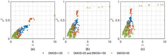
Figure 1. 2D scatter plots between GGD parameters $\alpha$ and ${\sigma }^2$ of the three NFMs, where each point in the scatter plots represents one distorted image in LIVE [28] database: (a) scatter plots for the first NFM; (b) scatter plots for the second NFM; and (c) scatter plots for the third NFM.

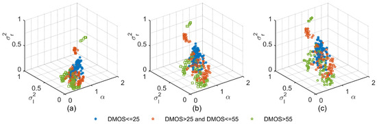
Figure 2. 3D scatter plots between AGGD parameters $\alpha$, ${\sigma }_l^2$ and ${\sigma }_r^2$ in horizontal orientation of the three NFMs, where each point in the scatter plots represent one distorted image in LIVE [28] database: (a) scatter plots for the first NFM; (b) scatter plots for the second NFM; and (c) scatter plots for the third NFM.

2.2. Correlation Coefficient between Adjacent Pixels in NFMs

There are strong structural correlations among neighboring pixels [15]. By examining the relationship between neighboring pixels in the NFMs, we found that the presence of distortions will alter the global correlation between spatially adjacent pairs in natural images. PLCC is employed to quantify the correlation changes between adjacent pairs in the NFMs. The four PLCC values along horizontal ($p_{\mathrm{H}}$), vertical ($p_{\mathrm{V}}$), main-diagonal ($p_{\mathrm{MD}}$) and secondary-diagonal ($p_{\mathrm{SD}}$) orientations are calculated by

$$p_{i,\mathrm{H}}=P(T_i(1:M,1:N-1),T_i(1:M,2:N))$$

(6)

$$p_{i,\mathrm{V}}=P(T_i(1:M-1,1:N),T_i(2:M,1:N))$$

(7)

$$p_{i,\mathrm{MD}}=P(T_i(1:M-1,1:N-1),T_i(2:M,2:N))$$

(8)

$$p_{i,\mathrm{SD}}=P(T_i(2:M,1:N-1),T_i(1:M,2:N))$$

(9)

where $T_i$ is the ith NFMs, $i\in 1,2,3$ is the NFM index, M and N are the height and the width of NFMs, respectively, and

$$P(X,Y)=\frac{{\displaystyle \sum _{m=1}^M}{\displaystyle \sum _{n=1}^N}(x_{m,n}-\overline{X})(y_{m,n}-\overline{Y})}{\sqrt{{\displaystyle \sum _{m=1}^M}{\displaystyle \sum _{n=1}^N}{(x_{m,n}-\overline{X})}^2{\displaystyle \sum _{m=1}^M}{\displaystyle \sum _{n=1}^N}{(y_{m,n}-\overline{Y})}^2}}$$

(10)

where X and Y are two non-overlapping blocks with equal size of the NFM, $\overline{X}$ and $\overline{Y}$ are the mean values of X and Y, $m\in 1,2,\cdots ,M$ and $n\in 1,2,\cdots ,N$ are the pixels indices, and M and N are the blocks height and width, respectively.

To illustrate how distortion types and distortion levels will affect the PLCC values between adjacent pairs, we take images in CSIQ database [29] as an example. Figure 3 plots the PLCC values between neighboring pixels of the first NFM along four orientations for six types of distorted images in CSIQ database. The six distortion types are additive Gaussian white noise (WN), JPEG2000 compression (JP2K), JPEG compression (JPEG), pink Gaussian noise (PGN), Gaussian blur (GB), and global contrast decrements (GCD). Each distortion type contains four distorted images with different difference mean opinion scores (DMOS) values. The DMOS value of CSIQ database is in the range [0, 1], where higher scores represent lower quality. In Figure 3, we plot the curve of PLCC values varying with DMOS values for the first NFM for each type of distorted images and for the reference images, where DMOS = 0 corresponding to PLCC values of the reference images. It is clear that the PLCC values of WN and PGN images decrease gradually as the DMOS value increases, while the PLCC values of JPEG, JP2K and GB images increase significantly as the DMOS value increases. This implies that the PLCC values between spatially adjacent pixels can well characterize the presence of distortions.

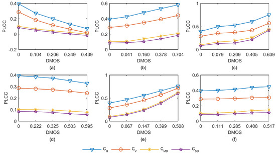
Figure 3. Variation of the PLCC values along four orientations for six types of distorted images in CSIQ database [29]. Each distortion type contains four distorted images with different difference mean opinion scores (DMOS) values, where DMOS = 0 corresponding to PLCC values of the pristine image: (a) additive Gaussian white noise (WN) distorted images; (b) JPEG compressed (JPEG) images; (c) JPEG2000 compressed (JP2K) images; (d) pink Gaussian noise (PGN) distorted images; (e) Gaussian blurred (GB) images; and (f) global contrast decrements (GCD) images.

Furthermore, we measure the PLCC values along four orientations for all the reference and distorted images in CSIQ database to more precisely describe the effect of the presence of distortions. Table 1 lists the average values of PLCC values along four orientations for each distortion type and the reference images. It is clear that the average PLCC values of different distortion types are quite different with the average PLCC values of the reference images. The average PLCC values of WN and PGN images are smaller than the average PLCC values of the reference images. The main reason is that there are many random signals in WN and PGN images, which will increase the differences between neighboring pixels and will also reduce the correlation between neighboring pairs. Besides, the average PLCC values of JPEG, JP2K, and GB images are much larger than the average PLCC values of the reference images. This is because less detailed information is contained in the compressed and blurred images, which will reduce the differences between neighboring pixels and will make the correlation between neighboring pairs larger. Moreover, since the global contrast decreasing will not change the correlation between adjacent pixels, the average PLCC values of GCD images are similar with the average PLCC values of the reference images. The experimental result implies that the PLCC values between spatially adjacent pixels can well characterize the presence of distortions.

Table 1. The average PLCC values along four orientations for the reference images and each type of distorted images in CSIQ database [29].

Distortion	${\mathit{p}}_{1,\mathbf{H}}$	${\mathit{p}}_{1,\mathbf{V}}$	${\mathit{p}}_{1,\mathbf{MD}}$	${\mathit{p}}_{1,\mathbf{SD}}$
Reference	0.3238	0.2689	0.0595	0.0600
WN	0.0902	0.0650	0.0086	0.0122
JPEG	0.4698	0.3991	0.1049	0.1041
JP2K	0.5367	0.4695	0.2773	0.2746
PGN	0.2821	0.2437	0.0430	0.0407
GB	0.5495	0.4930	0.3401	0.3359
GCD	0.3366	0.2781	0.0693	0.0705

2.3. Difference between NFMs

Since different NFMs contain different information from receptive fields of different sizes, we calculate the differential feature map (DFM) between NFMs to measure more detailed information of image degradation. The DFM between two NFMs is calculated by

$$D_i(m,n)=|{\left(T_i(m,n)\right)}^2-{\left(T_{i+1}(m,n)\right)}^2|$$

(11)

where $D_i$ are the ith DFMs, $T_i$ and $T_{i+1}$ are two different NFMs, $m\in 1,2,\cdots ,M$ and $n\in 1,2,\cdots ,N$ are the pixels indices, M and N are the image height and width, respectively, and $i\in 1,2$ is the index of the DFMs.

Our hypothesis is that the presence of distortions may affect the distribution properties of the DFMs, and measuring the distribution statistics in DFMs may better characterize image degradation. To visualize how the presence of distortions will affect the distributions of DFMs, we use five distorted images of different mean opinion score (MOS) values in the LIVE In the Wild Image Quality Challenge Database (WIQCD) [30] as an example. The MOS value of WIQCD database is in the range [0, 100], where higher scores represent higher quality. Figure 4 gives the five images in WIQCD database. Figure 5a visualizes the distributions of the DFMs between $T_1$ and $T_2$ for the five distorted images showed in Figure 4. It can be seen in Figure 5a that histograms of these DFMs follow the Weibull distribution, while the peak and tails of the five histograms are different. Therefore, we use Weibull model to fit the distribution of the DFMs. The probability density function associated with Weibull model is defined as

$$f(x_i;a_i,b_i)=\frac{b_i}{a_i}{\left(\frac{x_i}{a_i}\right)}^{b_i-1}\exp \left(-{\left(\frac{x_i}{a_i}\right)}^{b_i}\right),x_i>0$$

(12)

where $a_i$ and $b_i$ are the scale parameter and shape parameter of the ith DFM, respectively, and $i\in 1,2$ is the index of DFMs.

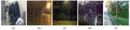
Figure 4. The five distorted images in the WIQCD database [30]: (a) MOS = 25.33; (b) MOS = 35.89; (c) MOS = 48.94; (d) MOS = 54.58; and (e) MOS = 66.51.

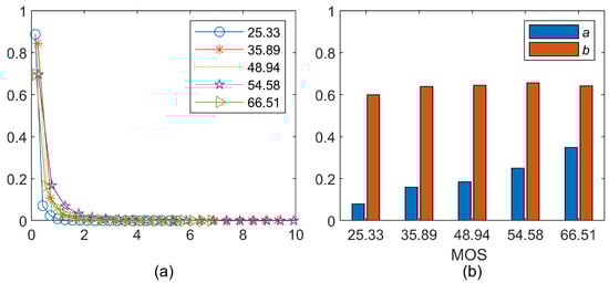
Figure 5. Distributions of the DFMs follow the Weibull distribution, and the distribution statistics of the DFMs increase as the MOS value grows: (a) distributions; and (b) bar plots of a and b.

Figure 5b gives bar plots of $a_1$ and $b_1$ of the five histograms shown in Figure 5a. It is clear that $a_1$ and $b_1$ increase as the MOS value grows. This indicates that the distribution statistics of the DFMs can measure the quality variation and can be adopted as perceptual features.

2.4. Statistics in Color Space

Color is also an important ingredient for visual quality perception [31]. De et al. [32] investigated the important role that color information played in image quality prediction. Redi et al. [33] utilized the color distribution features for reduced-reference IQA algorithm. Temel et al. [1] proposed an unsupervised learning approach that utilized the structural information in the YCbCr color space to improve the prediction accuracy of image quality. However, only a few BIQA algorithms concerned about the effect of color information. Considering the HSV color space, which contains the three components hue, saturation, and lightness, provides an intuitive representation of color and is more suitable than the RGB color space to capture features correlate well with human perception, we employ the color entropy and the low-level statistics of the three channels in the HSV color space as a complement to the gray-scale features.

Visual entropy can effectively measure the uncertainty of an image, and can be utilized to quantify the distorted information [34,35]. Therefore, we employ the color entropy of the three channels in the HSV space to characterize color information. The entropy of the kth channel is calculated by

$$E^k=\sum _{i=0}^{255}{p}_i^k{log}_2{p}_i^k$$

(13)

where $p_i^k$ is the probability density of ith level in kth channel, $k\in 1,2,3$.

Image gradient magnitude is sensitive to the degradations of images [19,36,37]. Therefore, before calculating the low-level statistics for the HSV color space, we compute the gradient magnitude map for each channel in the HSV color space. The gradient magnitude map of kth channel is computed by

$$G{M}^k=\sqrt{{[I^k(x,y)\ast G_h]}^2+{[I^k(x,y)\ast G_v]}^2}$$

(14)

where * is the linear convolution operator, $I^k(x,y)$ denotes the map of the kth channel in the HSV color space, and $G_h$ and $G_v$ are the Gaussian partial derivative filters applied along the horizontal (h) and vertical (v) directions. Here, the Gaussian partial derivative filter is used as convolution masks to perform a local averaging to reduce the effects of noise in the HSV color space, and can be defined as

$$G_d=\frac{\partial }{\partial d}g(x,y|\sigma )=-\frac{1}{2\pi {\sigma }^2}\frac{d}{{\sigma }^2}\exp \left(-\frac{x^2+y^2}{2{\sigma }^2}\right),d\in (h,v)$$

(15)

where $\sigma$ is the scale parameter of the Gaussian function $g(x,y|\sigma )$.

Figure 6 shows how the 3D scatter plots of the mean, the standard deviation, and the entropy of each channel in the HSV color space distributed in the feature space, where each point in the scatter plots represents one distorted image in LIVE database. We can see clearly that the distorted images belonging to different categories of DMOS values occupy different regions of the feature space, which means that the color features extracted from the HSV color space can help to distinguish images of different quality scores.

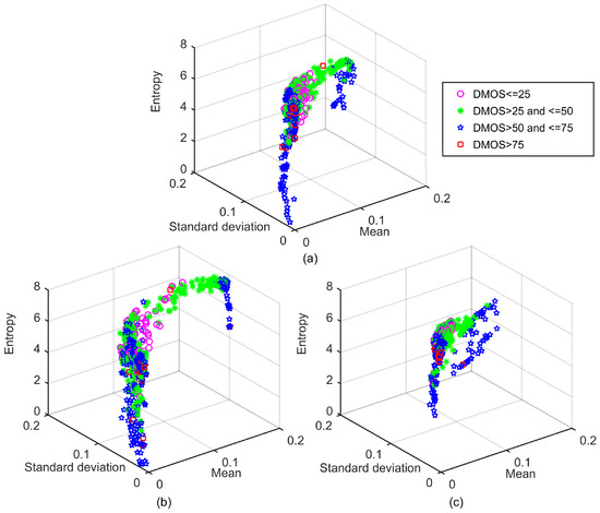
Figure 6. 3D scatter plots between the color features extracted from HSV color space on LIVE [28] database: (a) features in the saturation channel; (b) features in the hue channel; and (c) features in the value channel.

2.5. Statistical Features and Evaluation Model

Considering the computational complexity and the accuracy performance, three Gaussian windows (with $K=L=2,4,6$) are employed in the proposed BIQA-SC. For a given image, three NFMs and two DFMs can be obtained. Statistics including GGD parameters, AGGD parameters, and PLCC values among neighboring pixels are extracted from the three NFMs. The Weibull parameters are computed for the two DFMs. To achieve a better performance, the above features are extracted from the original resolution and a reduced resolution (down-sampled by a factor of 2). The color features are only extracted from the original resolution.

To comprehensively investigate the effectiveness of the proposed method, we train three support vector machine regressor (SVR) models by using different feature sets for estimating the perceptual quality score. We use only GGD and AGGD parameters extracted from the multiple NFMs to train the first SVR model, which is denoted by BIQA-SC-I. In the second model, which is denoted by BIQA-SC-II, GGD and AGGD parameters, PLCC values, and Weibull parameters are used to train the evaluation model. In the third model, which is denoted by BIQA-SC, all features extracted from the NFMs, the DFMs, and the HSV color space are used to train the evaluation model. The LIBSVM package [38] is utilized to implement the SVR models, and the radial basis function is employed as the regression kernel.

3. Experiments and Results

3.1. Databases and Evaluation Methodology

We evaluated the performance of the proposed algorithm on six benchmark IQA databases: LIVE [28], TID2013 [39], CSIQ [29], LIVE multiply distorted database I (MD1) [40], LIVE multiply distorted database II (MD2) [40], and WIQCD [30]. LIVE database includes 29 reference images and 779 distorted images of five distortion types. TID2013 database consists of 25 pristine images and 3000 distorted images with 24 distortion types. CSIQ database contains 30 reference images and 866 distorted images with six distortion types. MD1 database includes 225 images distorted by blur and JPEG. MD2 database includes 225 images distorted by blur and noise. WIQCD database consists of 1169 widely diverse authentic distorted images. It is worth mentioning that images in WIQCD database are directly obtained by using a lot of highly different smart phones and tablets, and the distorted images are totally different from each other because they are authentically distorted images acquired from typical real scenes.

Three commonly used performance metrics, i.e., the Spearman rank-order correlation coefficient (SROCC), the PLCC, and the root mean square error (RMSE), were employed to evaluate the competing BIQA algorithms. A better BIQA algorithm is expected to have lower RMSE value and higher values of SROCC and PLCC.

3.2. Overall Performance Comparison

The proposed algorithms were evaluated in comparison with the state-of-the-art BIQA algorithms including DIIVINE [12], BLIINDS-II [13], BRISQUE [15], ILNIQE [17], and GMLOG [19]. The overall performance on individual databases in terms of SROCC, PLCC, and RMSE are listed in Table 2. For each performance measure, the two best algorithms are highlighted in boldface.

Table 2. The median of SROCC, PLCC, and RMSE across the 1000 train-test trials on individual databases. The best two performances in terms of SROCC, PLCC, and RMSE are highlighted in boldface.

Metric	Algorithm	LIVE	TID2013	CSIQ	MD1	MD2	WIQCD
	DIIVINE [12]	0.941	0.824	0.895	0.932	0.876	0.561
	BLIINDS-II [13]	0.885	0.793	0.822	0.665	0.015	0.496
	BRISQUE [15]	0.933	0.805	0.794	0.933	0.878	0.605
SROCC	ILNIQE [17]	0.847	0.494	0.804	0.891	0.882	0.440
	GMLOG [19]	0.948	0.828	0.849	0.908	0.832	0.597
	BIQA-SC-I	0.948	0.837	0.881	0.899	0.921	0.632
	BIQA-SC-II	0.954	0.844	0.910	0.962	0.951	0.667
	BIQA-SC	0.956	0.906	0.928	0.957	0.964	0.682
	DIIVINE [12]	0.941	0.844	0.885	0.943	0.904	0.565
	BLIINDS-II [13]	0.866	0.832	0.835	0.691	0.073	0.529
	BRISQUE [15]	0.934	0.833	0.826	0.953	0.909	0.621
PLCC	ILNIQE [17]	0.620	0.509	0.724	0.834	0.852	0.491
	GMLOG [19]	0.952	0.849	0.857	0.933	0.866	0.612
	BIQA-SC-I	0.950	0.857	0.881	0.923	0.931	0.661
	BIQA-SC-II	0.955	0.869	0.904	0.971	0.959	0.682
	BIQA-SC	0.958	0.909	0.917	0.969	0.968	0.696
	DIIVINE [12]	5.510	0.675	0.125	6.452	8.097	17.685
	BLIINDS-II [13]	12.91	0.710	0.149	19.15	27.08	46.566
	BRISQUE [15]	5.777	0.694	0.152	5.915	7.879	16.125
RMSE	ILNIQE [17]	10.802	0.956	0.143	8.169	8.248	17.664
	GMLOG [19]	4.945	0.660	0.138	6.974	9.484	16.165
	BIQA-SC-I	5.073	0.641	0.125	7.478	6.9485	15.446
	BIQA-SC-II	4.778	0.623	0.115	4.668	5.361	15.020
	BIQA-SC	4.623	0.522	0.106	4.775	4.765	14.625

In the experiments, although there are pristine images in some databases, we only used distorted images for training and testing. Each database was randomly divided into a training subset and a test subset without overlapping, where the training subset contained $80\%$ of distorted images in the database and the test subset contained the remaining $20\%$ of distorted images in the database. To eliminate the performance bias, this train-test procedure was implemented for 1000 times, and the median values across 1000 trials were taken as the final performance evaluation.

It can be observed in Table 2 that the proposed algorithms achieved encouraging results on all the databases. The top two algorithms were BIQA-SC-II and BIQA-SC, which indicates that the proposed algorithms correlate well with human subjective judgements of image quality on all the databases. In terms of the three performance metrics, BIQA-SC-II had similar results to BIQA-SC on LIVE, CSIQ, MD1, and MD2 databases, and was obviously inferior to BIQA-SC on TID2013 and WIQCD databases. The proposed BIQA-SC-II, which employs the correlation statistics and Weibull parameters, was better than BIQA-SC-I, which employs only the GGD and AGGD parameters extracted from the NFMs. The comparison results demonstrate that the multiple NFMs, the DFMs, and the HSV color image contain useful information for characterizing the perception quality of images with various distortion types.

For the purpose of evaluating the statistical significance between BIQA-SC and other competing BIQA algorithms, a t-test was conducted at 95% significance level between the SROCC results generated by the competing algorithms across the 1000 train-test trials. The results of the t-test are shown in Table 3. The symbol 1 (−1) indicates that BIQA-SC is statistically superior (inferior) to the compared algorithm, and 0 indicates that BIQA-SC and the compared algorithm are statistically indistinguishable. It can be seen that BIQA-SC was superior to all the compared algorithms on all the databases.

Table 3. Results of the t-test between the SROCC results generated by the competing algorithms across the 1000 train-test trials on benchmark databases. The symbols 1, −1, and 0 indicate that BIQA-SC is statistically superior, inferior, or indistinguishable to the compared algorithm.

Algorithm	LIVE	TID2013	CSIQ	MD1	MD2	WIQCD
DIIVINE [12]	1	1	1	1	1	1
BLIINDS-II [13]	1	1	1	1	1	1
BRISQUE [15]	1	1	1	1	1	1
ILNIQE [17]	1	1	1	1	1	1
GMLOG [19]	1	1	1	1	1	1
BIQA-SC-I	1	1	1	1	1	1
BIQA-SC-II	1	1	1	−1	1	1

To visualize the statistical significance comparison, Figure 7 shows the box plots of the SROCC and PLCC distributions of the competing BIQA algorithms over 1000 train-test trials on LIVE database. It is clear that the quality scores produced by the proposed BIQA-SC correlated well with human subjective opinions on LIVE database. The proposed BIQA-SC was statistically superior to the state-of-the-art BIQA approaches. The scatter plots and the fitted lines of the DMOS values versus the scores predicted by the competing methods are shown in Figure 8. It can be observed that the predicted scores of the proposed BIQA-SC were nearly linear with the DMOS.

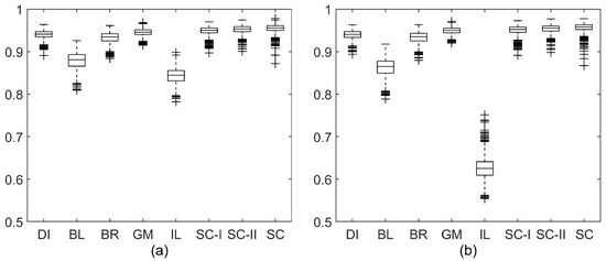
Figure 7. Box plots of SROCC and PLCC distributions of BLIINDS-II [13] (BL), DIIVINE [12] (DI), BRISQUE [15] (BR), GMLOG [19] (GM), BIQA-SC-I (SC-I), BIQA-SC-II (SC-II), and BIQA-SC (SC) across 1000 train-test trials on LIVE database [28]: (a) box plot of SROCC distributions; and (b) box plot of PLCC distributions.

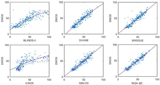
Figure 8. Scatter plots and fitted lines of the DMOS values versus the predicted scores by the competing algorithms on LIVE database [28].

3.3. Performance on Individual Distortion Types

To fully test the proposed algorithm, we also compared the performance of the competing BIQA algorithms on individual distortion types in LIVE and CSIQ databases. The same train-test procedures as in the previous experiments were conducted. The median SROCC values across the 1000 train-test trials are listed in Table 4. It is clear that most of the competing algorithms could achieve good evaluation accuracy on individual distortion types in LIVE database. However, only BIQA-SC and BIQA-SC-II could obtain relatively high prediction accuracy on each distortion type in CSIQ database. Compared with BRISQUE [15], which only utilizes NSS features extracted from a single NFM, BIQA-SC-I and BIQA-SC-II had significantly improved prediction accuracy on six types of distortions in CSIQ database. This implies that statistics extracted from multiple NFMs and DFMs are more sensitive to the distortion changes than statistics obtained from a single NFM. The main reason is that measuring the relationship between coefficients in receptive fields of different sizes could get more detailed information indicating the changes of the surrounding world. Moreover, BIQA-SC achieved the best performance on individual distortion types in CSIQ database. This implies that using color features extracted from HSV color space can improve the evaluation accuracy of contrast distorted images.

Table 4. Median SROCC comparison of the competing algorithms on individual distortion types in LIVE [28] and CSIQ [29] databases. The distortion types include additive Gaussian white noise (WN), JPEG compression (JPEG), JPEG2000 compression (JP2K), Gaussian blur (GB), fast fading (FF), pink Gaussian noise (PGN), and global contrast decrements (GCD). The best two algorithms are highlighted in boldface.

Algorithm	LIVE					CSIQ
	JP2K	JPEG	WN	GB	FF	WN	JPEG	JP2K	PGN	GB	GCD
DIIVINE [12]	0.911	0.911	0.977	0.955	0.911	0.909	0.883	0.883	0.941	0.889	0.886
BLIINDS-II [13]	0.916	0.886	0.959	0.910	0.834	0.776	0.778	0.839	0.828	0.882	0.685
BRISQUE [15]	0.913	0.908	0.973	0.960	0.869	0.861	0.850	0.834	0.868	0.863	0.447
ILNIQE [17]	0.872	0.863	0.980	0.916	0.833	0.851	0.875	0.894	0.877	0.830	0.518
GMLOG [19]	0.917	0.930	0.981	0.934	0.918	0.704	0.864	0.878	0.881	0.872	0.833
BIQA-SC-I	0.928	0.918	0.982	0.967	0.908	0.934	0.891	0.849	0.926	0.907	0.886
BIQA-SC-II	0.939	0.911	0.983	0.966	0.915	0.931	0.888	0.908	0.939	0.916	0.919
BIQA-SC	0.938	0.913	0.985	0.973	0.915	0.943	0.911	0.924	0.967	0.940	0.950

To further test the generalization ability of the proposed algorithms, we also conducted experiments on the 24 distortion types in TID2013 database. The bar plots in Figure 9 correspond to the median SROCC values of 1000 train-test trials on TID2013 database. It is clear that BIQA-SC achieved promising results on most commonly encountered distortion types. For several special distortion types, such as local block-wise distortion (LBD), contrast change (CC), change of color saturation (CCS), and comfort noise (CN), BIQA-SC still achieved satisfying results and outperformed state-of-the-art algorithms. This indicates that the proposed method is capable of evaluating the image quality for various distortion types.

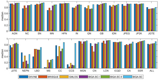
Figure 9. Median SROCC results of 1000 train-test trials on TID2013 database [39] for DIIVINE [12], BRISQUE [15], GMLOG [19], BIQA-SC-I, BIQA-SC-II and BIQA-SC. There are 24 distortion types in TID2013 [39] database, including additive Gaussian noise (AGN), additive noise in color components is more intensive than additive noise in the luminance component (NC), spatially correlated noise (SN), masked noise (MN), high frequency noise (HFN), impulse noise (IN), quantization noise (QN), Gaussian blur (GB), image denoising (IDN), JPEG compression (JPEG), JPEG2000 compression (JP2K), JPEG transmission errors (JPTE), JPEG2000 transmission errors (J2TE), non eccentricity pattern noise (NEPN), local block-wise distortions of different intensity (LBD), mean shift (MS), contrast change (CC), change of color saturation (CCS), multiplicative Gaussian noise (MGN), comfort noise (CN), lossy compression of noisy images (LCN), image color quantization with dither (ICQD), chromatic aberrations (CA), and sparse sampling and reconstruction (SSR).

3.4. Impact of Varying the Number of NFMs

As shown in Table 5, we examined how the number of the NFMs used in BIQA-SC would be affected the performance. We denote BIQA-SC using $n(n\in 1,2,\cdots ,5$) NFMs as Mn. It can be seen that better performance in terms of RMSE, SROCC, and PLCC is likely to be achieved if multiple NFMs are used. However, the prediction performance does not improve too much when the number of the NFMs is larger than 3 on most of the databases. To better analyze the difference between the BIQA-SC using different numbers of the NFMs, we calculated the statistical significance between each two of the Mn algorithms by conducting a t-test at 95% significance level between SROCC values of these algorithms across the 1000 train-test iterations. The t-test results are shown in Table 6. The symbol 1 (−1) indicates that the algorithm in the row is statistically superior (inferior) to the algorithm in the column, and 0 indicates that the two compared algorithms are statistically indistinguishable. Clearly, M3, M4, and M5 were superior to M1 and M2 on nearly all databases, while M3, M4, and M5 achieved better evaluation performance on different database. Considering the balance of performance and computational cost, we use three NFMs in the proposed BIQA-SC.

Table 5. Median SROCC of BIQA-SC on six databases when using different numbers of NFMs, where BIQA-SC using $n(n\in 1,2,\cdots ,5$) NFMs is denoted as Mn.

Metric	K and L	Metric	LIVE	TID2013	CSIQ	MD1	MD2	WIQCD
M1	2	SROCC	0.949	0.880	0.927	0.945	0.950	0.644
		PLCC	0.951	0.889	0.919	0.959	0.955	0.655
		RMSE	5.008	0.576	0.106	5.500	5.607	15.436
M2	2,4	SROCC	0.953	0.900	0.932	0.952	0.958	0.660
		PLCC	0.956	0.903	0.923	0.965	0.963	0.676
		RMSE	4.772	0.533	0.103	5.093	5.084	15.209
M3	2,4,6	SROCC	0.956	0.906	0.928	0.957	0.964	0.682
		PLCC	0.958	0.909	0.917	0.969	0.968	0.696
		RMSE	4.623	0.522	0.106	4.775	4.765	14.63
M4	2,4,6,8	SROCC	0.956	0.900	0.927	0.956	0.966	0.672
		PLCC	0.958	0.904	0.918	0.968	0.970	0.689
		RMSE	4.638	0.532	0.107	4.813	4.616	14.989
M5	2,4,6,8,10	SROCC	0.952	0.906	0.930	0.958	0.963	0.669
		PLCC	0.955	0.908	0.921	0.969	0.968	0.685
		RMSE	4.812	0.522	0.105	4.751	4.719	14.911

Table 6. Statistical significance comparison of M1, M2, M3, M4, and M5 with t-test between SROCC values of Mn algorithms on six databases, where BIQA-SC using $n(n\in 1,2,\cdots ,5$) NFMs is as Mn.

	LIVE					TID2013					CSIQ
Metric	M1	M2	M3	M4	M5	M1	M2	M3	M4	M5	M1	M2	M3	M4	M5
M1	0	−1	−1	−1	−1	0	−1	−1	−1	−1	0	−1	0	0	−1
M2	1	0	−1	−1	0	1	0	−1	0	−1	1	0	1	1	0
M3	1	1	0	1	1	1	1	0	1	0	0	−1	0	0	−1
M4	1	1	−1	0	1	1	0	−1	0	−1	0	−1	0	0	−1
M5	1	0	−1	−1	0	1	1	0	1	0	1	0	1	1	0
	MD1					MD2					WIQCD
Metric	M1	M2	M3	M4	M5	M1	M2	M3	M4	M5	M1	M2	M3	M4	M5
M1	0	−1	−1	−1	−1	0	−1	−1	−1	−1	0	−1	−1	−1	−1
M2	1	0	−1	−1	−1	1	0	−1	−1	−1	1	0	−1	0	0
M3	1	1	0	1	0	1	1	0	−1	−1	1	1	0	0	0
M4	1	1	−1	0	−1	1	1	1	0	1	1	0	0	0	0
M5	1	1	0	1	0	1	1	1	−1	0	1	0	0	0	0

3.5. Cross Database Experiments

Cross-database experiments were also carried out to investigate the generalization ability and robustness of BIQA-SC. In the experiments, we used one database as training set and the other databases as testing sets. In Table 7, we list the SROCC of the competing algorithms when these algorithms were trained on LIVE database and tested on the other databases. The two best algorithms are highlighted in boldface. It can be seen in Table 7 that the performance of all the competing algorithms decreased significantly compared with their performance on individual databases. The main reason is that there are only five distortion types in LIVE database while the testing databases contain many other types of distortions, such as contrast distortion, multiple distortions, color distortions, etc. Moreover, only TID2013 and LIVE databases contain partial images of the same scene. The images in other databases are completely different from those in LIVE database. Nevertheless, BIQA-SC still performed well compared to the competing algorithms. Besides, we also trained the competing algorithms on the entire TID2013 database, and tested them on the other databases. The experimental results shown in Table 8 demonstrate that BIQA-SC is database independent and outperformed the other competing algorithms.

Table 7. The SROCC of the competing algorithms when trained on LIVE database [28]. The best two algorithms are highlighted in boldface.

Algorithm	TID2013	CSIQ	MD1	MD2	WIQCD
DIIVINE [12]	0.414	0.569	0.772	0.655	0.357
BLIINDS-II [13]	0.319	0.535	0.731	0.355	0.143
BRISQUE [15]	0.457	0.472	0.733	0.224	0.332
GMLOG [19]	0.468	0.547	0.563	0.309	0.218
BIQA-SC	0.469	0.497	0.741	0.451	0.323

Table 8. The SROCC of the competing algorithms when trained on TID2013 database [39]. The best two algorithms are highlighted in boldface.

Algorithm	LIVE	CSIQ	MD1	MD2	WIQCD
DIIVINE [12]	0.680	0.456	0.679	0.447	0.170
BLIINDS-II [13]	0.681	0.426	0.660	0.098	0.085
BRISQUE [15]	0.740	0.499	0.521	0.472	0.280
GMLOG [19]	0.812	0.591	0.541	0.019	0.121
BIQA-SC	0.748	0.584	0.719	0.475	0.160

3.6. Computational Cost Comparison

Table 9 lists the average feature extraction cost of an image in LIVE database for all competing algorithms. All the results were measured in seconds with Matlab2014b implementation on a desktop computer with 2.7 GHz Intel Core i7 CPU and 16GB RAM. As shown in Table 9, the three most efficient algorithms were BRISQUE [15], GMLOG [19], and the proposed BIQA-SC, while DIIVINE [12] and BLIINDS-II [13] had the highest cost. The main reason for such big differences in computational cost is that the image transformation and feature extraction strategies adopted by the competing algorithms are quite different. In DIIVINE [12], the scale-space-orientation decomposition of the distorted image and the GGD fitting procedure for each wavelet subband slow down the approach greatly. The block-based method BLIINDS-II [13] needs to perform local discrete cosine transformation and complex feature extraction strategies for each block, which will inevitably lead to high computational complexity. Different from DIIVINE [12] and BLIINDS-II [13], BRISQUE [15] is based on spatial domain, thus it does not need to perform complex image transformation. Similarly, GM-LOG [19] only employs gradient and Laplacian Gaussian features, which costs very short computational time. Compared with BRISQUE and GM-LOG algorithms, the proposed BIQA-SC that extracts statistics from multiple NFMs, DFMs, and color space needs a little more computational time, but the performance of BIQA-SC is greatly improved. In short, the experimental results in Table 2, Table 3, Table 4, Table 5, Table 6, Table 7, Table 8 and Table 9 prove that BIQA-SC has the best performance on all the databases and has a relatively low computational cost, which makes BIQA-SC more suitable for practical application.

Table 9. Comparison of computation time on LIVE [28] database. The best two algorithms are highlighted in boldface.

Metric	DIIVINE [12]	BLIINDS-II [13]	BRISQUE [15]	ILNIQE [17]	GMLOG [19]	BIQA-SC
Time (s)	19.24	70.70	0.09	4.90	0.07	0.82

4. Conclusions

In this paper, we extract statistical features from the spatial and the color domains to form a powerful quality-aware feature vector for image quality pooling. By using the multi-window method, the proposed BIQA-SC algorithm can better characterize the degradations in the distorted images from receptive fields of different sizes. Quantifying the correlation between adjacent coefficients in the multiple NFMs, and measuring the difference between different NFMs can also improve the prediction accuracy of the image quality. The color entropy and the low-level gradient statistics extracted from the HSV color space make BIQA-SC capable of evaluating the quality more accurately for a variety of distorted images. Experimental results on LIVE, TID2013, CSIQ, MD1, MD2, and WIQCD databases show that BIQA-SC can considerably improve the prediction accuracy on a broad range of synthetically distorted images as well as authentically distorted images. BIQA-SC performs much better than state-of-the-art algorithms with relatively low computational cost, which makes it more suitable for practical applications.

References

- Temel, D.; Prabhushankar, M.; AlRegib, G. UNIQUE: Unsupervised image quality estimation. IEEE Signal Process. Lett. 2016, 23, 1414–1418. [Google Scholar] [CrossRef]
- Prabhushankar, M.; Temel, D.; AlRegib, G. MS-UNIQUE: Multi-model and sharpness-weighted unsupervised image quality estimation. Electron. Imaging 2017, 12, 30–35. [Google Scholar]
- Li, Q.; Lin, W.; Fang, Y. No-reference quality assessment for multiply-distorted images in gradient domain. IEEE Signal Process. Lett. 2016, 23, 541–545. [Google Scholar] [CrossRef]
- Zhang, H.; Yuan, B.; Dong, B.; Jiang, Z. No-Reference Blurred Image Quality Assessment by Structural Similarity Index. Appl. Sci. 2018, 8, 2003. [Google Scholar] [CrossRef]
- Bosse, S.; Maniry, D.; Müller, K.R.; Wiegand, T.; Samek, W. Deep neural networks for no-reference and full-reference image quality assessment. IEEE Trans. Image Process. 2018, 27, 206–219. [Google Scholar] [CrossRef] [PubMed]
- He, L.; Gao, X.; Lu, W.; Li, X.; Tao, D. Image quality assessment based on S-CIELAB model. Signal Image Video Process. 2011, 5, 283–290. [Google Scholar] [CrossRef]
- Saha, A.; Wu, Q.J. Perceptual image quality assessment using phase deviation sensitive energy features. Signal Process. 2013, 93, 3182–3191. [Google Scholar] [CrossRef]
- Cheng, G.; Huang, J.; Liu, Z.; Lizhi, C. Image quality assessment using natural image statistics in gradient domain. AEU-Int. J. Electron. Commun. 2011, 65, 392–397. [Google Scholar] [CrossRef]
- Sazzad, Z.P.; Kawayoke, Y.; Horita, Y. No reference image quality assessment for JPEG2000 based on spatial features. Signal Process. Image Commun. 2008, 23, 257–268. [Google Scholar] [CrossRef]
- Liu, H.; Klomp, N.; Heynderickx, I. A no-reference metric for perceived ringing artifacts in images. IEEE Trans. Circuits Syst. Video Technol. 2010, 20, 529–539. [Google Scholar] [CrossRef]
- Moorthy, A.K.; Bovik, A.C. A two-step framework for constructing blind image quality indices. IEEE Signal Process. Lett. 2010, 17, 513–516. [Google Scholar] [CrossRef]
- Moorthy, A.K.; Bovik, A.C. Blind image quality assessment: From natural scene statistics to perceptual quality. IEEE Trans. Image Process. 2011, 20, 3350–3364. [Google Scholar] [CrossRef] [PubMed]
- Saad, M.A.; Bovik, A.C.; Charrier, C. Blind image quality assessment: A natural scene statistics approach in the DCT domain. IEEE Trans. Image Process. 2012, 21, 3339–3352. [Google Scholar] [CrossRef] [PubMed]
- Zhang, Y.; Moorthy, A.K.; Chandler, D.M.; Bovik, A.C. C-DIIVINE: No-reference image quality assessment based on local magnitude and phase statistics of natural scenes. Signal Process. Image Commun. 2014, 29, 725–747. [Google Scholar] [CrossRef]
- Mittal, A.; Moorthy, A.K.; Bovik, A.C. No-reference image quality assessment in the spatial domain. IEEE Trans. Image Process. 2012, 21, 4695–4708. [Google Scholar] [CrossRef] [PubMed]
- Mittal, A.; Soundararajan, R.; Bovik, A.C. Making a completely blind image quality analyzer. IEEE Signal Process. Lett. 2013, 20, 209–212. [Google Scholar] [CrossRef]
- Zhang, L.; Zhang, L.; Bovik, A.C. A feature-enriched completely blind image quality evaluator. IEEE Trans. Image Process. 2015, 24, 2579–2591. [Google Scholar] [CrossRef]
- Ghadiyaram, D.; Bovik, A.C. Perceptual quality prediction on authentically distorted images using a bag of features approach. J. Vis. 2017, 17, 32. [Google Scholar] [CrossRef]
- Xue, W.; Mou, X.; Zhang, L.; Bovik, A.C.; Feng, X. Blind image quality assessment using joint statistics of gradient magnitude and laplacian features. IEEE Trans. Image Process. 2014, 23, 4850–4862. [Google Scholar] [CrossRef]
- Liu, L.; Hua, Y.; Zhao, Q.; Huang, H.; Bovik, A.C. Blind image quality assessment by relative gradient statistics and adaboosting neural network. Signal Process. Image Commun. 2016, 40, 1–15. [Google Scholar] [CrossRef]
- Zhou, W.; Yu, L.; Qiu, W.; Zhou, Y.; Wu, M. Local gradient patterns (LGP): An effective local-statistical-feature extraction scheme for no-reference image quality assessment. Inf. Sci. 2017, 397, 1–14. [Google Scholar] [CrossRef]
- Rezaie, F.; Helfroush, M.S.; Danyali, H. No-reference image quality assessment using local binary pattern in the wavelet domain. Multimed. Tools Appl. 2018, 77, 2529–2541. [Google Scholar] [CrossRef]
- Cai, H.; Li, L.; Yi, Z.; Gong, M. Towards a blind image quality evaluator using multi-scale second-order statistics. Signal Process., Image Commun. 2019, 71, 88–99. [Google Scholar] [CrossRef]
- Zhu, H.; Yu, S. Low-Illumination Image Enhancement Algorithm Based on a Physical Lighting Model. IEEE Trans. Circuits Syst. Video Technol. 2017, 29, 28–37. [Google Scholar]
- Nienborg, H.; Bridge, H.; Parker, A.J.; Cumming, B.G. Receptive field size in V1 neurons limits acuity for perceiving disparity modulation. J. Neurosci. 2004, 24, 2065–2076. [Google Scholar] [CrossRef]
- Lindeberg, T. A computational theory of visual receptive fields. Biol. Cybern. 2013, 107, 589–635. [Google Scholar] [CrossRef]
- Vonikakis, V.; Winkler, S. A center-surround framework for spatial image processing. Electron. Imaging 2016, 2016, 1–8. [Google Scholar] [CrossRef]
- Sheikh, H.; Wang, Z.; Cormack, L.; Bovik, A.C. LIVE Image Quality Assessment Database Release 2. 2005. Available online: http://live.ece.utexas.edu/research/quality (accessed on 17 July 2007).
- Larson, E.C.; Chandler, D.M. Most apparent distortion: full-reference image quality assessment and the role of strategy. J. Electron. Imaging 2010, 19, 011006. [Google Scholar]
- Ghadiyaram, D.; Bovik, A.C. Crowdsourced study of subjective image quality. In Proceedings of the 2014 48th Asilomar Conference on Signals, Systems and Computers, Pacific Grove, CA, USA, 2–5 November 2014; Volume 101, pp. 2008–2024. [Google Scholar]
- Jordan, J.R.; Geisler, W.S.; Bovik, A.C. Color as a source of information in the stereo correspondence process. Vis. Search 1990, 30, 1955–1970. [Google Scholar] [CrossRef]
- De Simone, F.; Dufaux, F.; Ebrahimi, T.; Delogu, C.; Baroncini, V. A subjective study of the influence of color information on visual quality assessment of high resolution pictures. In Proceedings of the 4th International Workshop on Video Processing and Quality Metrics for Consumer Electronics (VPQM-09), Scottsdale, AZ, USA, 15–16 January 2009. [Google Scholar]
- Redi, J.A.; Gastaldo, P.; Heynderickx, I.; Zunino, R. Color distribution information for the reduced-reference assessment of perceived image quality. IEEE Trans. Circuits Syst. Video Technol. 2010, 20, 1757–1769. [Google Scholar] [CrossRef]
- Sheikh, H.R.; Bovik, A.C.; De Veciana, G. An information fidelity criterion for image quality assessment using natural scene statistics. IEEE Trans. Image Process. 2005, 14, 2117–2128. [Google Scholar] [CrossRef] [PubMed]
- Liu, L.; Liu, B.; Huang, H.; Bovik, A.C. No-reference image quality assessment based on spatial and spectral entropies. Signal Process. Image Commun. 2014, 29, 856–863. [Google Scholar] [CrossRef]
- Zhang, L.; Zhang, L.; Mou, X.; Zhang, D. FSIM: A feature similarity index for image quality assessment. IEEE Trans. Image Process. 2011, 20, 2378–2386. [Google Scholar] [CrossRef] [PubMed]
- Xue, W.; Zhang, L.; Mou, X.; Bovik, A.C. Gradient magnitude similarity deviation: A highly efficient perceptual image quality index. IEEE Trans. Image Process. 2014, 23, 684–695. [Google Scholar] [CrossRef] [PubMed]
- Chang, C.C.; Lin, C.J. LIBSVM: A library for support vector machines. ACM Trans. Intell. Syst. Technol. (TIST) 2011, 2, 27. [Google Scholar] [CrossRef]
- Ponomarenko, N.; Jin, L.; Ieremeiev, O.; Lukin, V.; Egiazarian, K.; Astola, J.; Vozel, B.; Chehdi, K.; Carli, M.; Battisti, F. Image database TID2013: Peculiarities, results and perspectives. Signal Process. Image Commun. 2015, 30, 57–77. [Google Scholar] [CrossRef]
- Jayaraman, D.; Mittal, A.; Moorthy, A.K.; Bovik, A.C. Objective quality assessment of multiply distorted images. In Proceedings of the 46th Asilomar Conference on Signals, Systems and Computers (ASILOMAR), Pacific Grove, CA, USA, 4–7 November 2012; pp. 1693–1697. [Google Scholar]
© 2019 by the authors. Licensee MDPI, Basel, Switzerland. This article is an open access article distributed under the terms and conditions of the Creative Commons Attribution (CC BY) license (http://creativecommons.org/licenses/by/4.0/).