Evolution of b-Value and Fractal Dimension of Acoustic Emission Events During Shear Rupture of an Immature Fault in Granite

Abstract

The present study investigated the evolutions of b-value and fractal dimension of acoustic emission (AE) events during shear rupture of a naturally-created rough fracture in a granite specimen under triaxial compression. Acoustic emission signals were monitored by 16 sensors mounted directly on the surface of the specimen, and AE waveforms were sampled at 16 bits and 25 MHz. Reliable hypocenters were determined using P-wave arrival times picked up from the waveforms. Acoustic emission magnitude was determined from the maximum amplitude monitored by two peak detectors, which have a relative magnitude range of 0 to 2.75. A three-dimensional X-ray computed tomography scan was performed after the test to explore the fracture geometry. Acoustic emission activity was initiated during hydrostatic compression. With increasing differential stress, AEs demonstrated an increasing event rate, a decrease (from approximately 1.8 to 1.6) with a subsequent precursory increase (from 1.6 to 1.8) in fractal dimension, a quick decrease in b-value (from 1.0 to approximately 0.5), and a quick increase in fractal dimension (from 1.8 to 2.0). The exponentially increasing event rate, gradually decreasing b-value, and slowly increasing fractal dimension may be an intermediate-term indication of fault reactivation. In contrast, a progressively increasing event rate, a rapid drop in b-value, and a rapid increase in fractal dimension may facilitate short-term prediction of large events, which reflect the rupture of large patches. Acoustic emission hypocenters were clustered on the entire fracture surface. The present study sheds some light on detecting early signs of fault reactivation by monitoring injection-induced seismicity in areas with faults of different maturity.

1. Introduction

Injection-induced seismicity is a by-product in several scientific and industrial applications, such as tapping deep geothermal energy through an enhanced geothermal system (EGS), fracking shale gas, enhanced oil recovery (EOR), disposal of waste fluid, and geological storage of CO₂. Microseismicity can be used to monitor hydraulic fracturing and for reservoir management. However, felt events of magnitude (M) 2 and above near certain projects may have economic and social impacts [1], and repeated M ≥ 3 events may cause heavy damage, especially at seismically stable sites [2,3]. Under certain conditions, earthquake ruptures can be confined to pressurized regions. In contrast, under other conditions, earthquakes are able to propagate as sustained ruptures beyond the zone that experienced a pressure perturbation [4]. At sites without large-scale pre-existing faults, induced seismicity was limited in-zone (stimulated volume) and was mainly controlled by injection parameters, and thus induced seismicity could be better controlled because seismicity faded out quickly after shut-in. For such cases, as demonstrated by an EGS project, near–real-time seismic monitoring of fluid injection has allowed control of induced earthquakes via a well-designed traffic lighting system [5]. However, for worse cases encountered in damage events, major seismicity resulted from reactivation of large-scale pre-existing faults having different maturity [6,7]. Shear rupture of newly-created tensile fractures or pre-existing fractures opened by hydrofracturing is also a potential source inducing seismicity by later nearby injections [2,6]. Normally, earthquakes on immature faults produce stronger ground motions at all frequencies, as compared with that generated by earthquakes on mature faults [8]. A recent study showed that mature faults in basement and immature faults in sediments demonstrated seismically-different responses to injection operations [7]. Thus, the structural maturity of faults is an important parameter that should be considered, and the shear behaviors of faults having different maturities should be fully investigated at all scales. The possibility of detecting early signs of fault reactivation, which might be a function of structure maturity, is a key issue in risk assessment and hazard mitigation of injection-inducing seismicity.

Acoustic emission (AE) activity on a laboratory scale can be considered as microseismicity of a magnitude in the range of roughly from −11 to −4 [9]. Acoustic emission activity in stressed rocks shows similarities with seismicity in the crust via a number of power laws. The commonly accepted law is the Gutenberg and Richter (GR) relation for size distribution and fractal distribution of the AE hypocenter. Beginning with Mogi’s study published in 1962 [10], numerous laboratory studies have been motivated by the expectation that precursory changes in b-value may have resulted from stress changes and thus may be used for earthquake prediction and failure prediction in mines. Indeed, laboratory studies of AE events have consistently shown a decrease in b-value with increasing stress during the deformation of intact samples containing pre-existing microcracks e.g. Refs. [11,12,13,14,15].

In recent years, more studies have focused on AEs during frictional sliding on natural fractures/joints or pre-cut faults on laboratory scales because such set-ups provide a better analogue of fault rupture in nature. Systematic variations in b-value of the magnitude-frequency distribution of AE events were observed during stress buildup and release on laboratory-created fault zones [16] as well as during stable and unstable frictional sliding experiments on layers of glass beads in a double-direct shear configuration [17]. In a recent study, the results for unfavorably-oriented pre-cut faults showed similar behaviors: decreasing b-value followed by a quick jump prior to the stress drop for repeated stick-slip events [18]. As an integral set, the seismic b-value, together with parameters in other power laws, worked as an indicator of stress criticality [19]. Laboratory results have shed some light on detecting pre-failure signs of fault reactivation from seismicity. The present paper describes experimental results obtained during shear rupture of a granitic specimen containing a pre-existing natural fracture, which was an analogue of immature faults. By integrating seismic b-value into the magnitude-frequency distribution and fractal dimension (or spatial correlation length) in the AE hypocenter distribution, early signs of fault reactivation were examined.

2. Specimen, Experimental Setup, and Acoustic Emission Monitoring

2.1. Specimen Details

At first, a cylindrical specimen of 50 mm in diameter and 125 mm in length was cored from a granite block containing a macroscopic fracture. The fracture could be checked visually but was not completely penetrated and contained some unfractured small patches. The cylindrical specimens were cut along a direction so that the fracture was centered in the sample and had an angle of 32 degrees with respect to the axis, which was the direction of the greatest principal stress under the experimental conditions (Figure 1a). The granite was coarse grained and had a relatively high density of pre-existing microcracks, as indicated by a relatively lower initial P-wave velocity of approximately 4.5 km/s under room conditions. Similar, but microcrack-free, granites had an initial P-wave velocity greater than 6.0 km/s [20].

In total, 16 piezoelectric AE transducers (PZT) (diameter: 5 mm, resonant frequency: 2 MHz) were mounted using epoxy adhesive directly to the curvilinear surface of the sample for AE monitoring and velocity measurements (Figure 1b,e). The PZT transducers functioned not only as receivers of acoustic signals but also as detonators for measuring the P-wave velocity during the experiment. Six flat surfaces of a width of approximately 7 mm were prepared for better coupling between the flat transducers and the specimen (Figure 1a,b). In addition, seven pairs of cross-type strain gauges were placed on the curvilinear surface of the specimen in order to record local strains along the axial and circumferential directions. Then, the sample and two end pieces were coated with silicone sealant in order to prevent confining oil from leaking into the sample (Figure 1c).

2.2. Experimental Set-Up

The coated specimen was set with the vessel cover, which was equipped with a sufficient number of coaxial feedthroughs for connecting AE transducers and strain gauges with pre-amplifiers (Figure 1d). The specimen assembly was then placed in the pressure vessel within the loading cell (Figure 1f), which has a capacity of 20,000 kN. First, the specimen was isotropically (hydrostatically) compressed to a confining pressure of 40 MPa. The axial stress was then increased to 75 MPa at a rate of approximately 10 MPa/min under manual operation. Finally, the axial stress was increased at a constant rate of 2.25 MPa/min until failure. The peak axial stress was 220 MPa. When axial loading, the force was controlled by a spring-force balancing system, and the spring was simply compressed by a stepping motor. This loading system allowed dynamic fracturing and a quick stress drop.

2.3. Acoustic Emission Monitoring

Acoustic emission signals from the 16 PZTs were pre-amplified by 45 dB and then digitized at a sampling rate of 25 MHz and a sample length of 4096 words (approximately 160 microseconds) for each event. The A/D system had a dynamic range of 16 bits, 256 mega-words of onboard memory for each channel, and three working modes: single-event mode, multi-event mod, and continuous mode. In the single-event mode, the digitized waveform data of a triggered AE event were immediately transferred to the hard disk of the host PC. Since the system was able to record at most 10 events per second, the single-event mode was applied during the earlier stages of the experiment, when the AE rate was lower than 10 events per second. Once AE occurred more frequently, the system was switched to the multi-event mode, under which the system could record up to approximately 5000 events per second. All digitized waveform data were stored in the onboard memory, which had a capacity of 65,536 events under the aforementioned sampling conditions. Waveform data were finally transferred to the hard disk either when the onboard memory was full or the experiment was completed.

In addition to waveform recording, AE signals from two selected sensors (#3 and #10 in Figure 1e) were amplified by 20 dB and then fed to peak detectors (dynamic range: 100 dB) for event counting and recording the maximum amplitude of each event. The noise level for AE signals was approximately 40 dB after applying the 20-dB preamplifier. Thus, the threshold for the peak detectors was set to 45 dB, resulting in an effective dynamic range of 55 dB (corresponding to a relative magnitude range of from 0 to 2.75). A complicated triggering logic was designed for recording waveforms. First, three pairs of neighboring sensors were selected as triggering sensors (Figure 1e). In order to avoid biased triggering, the three pairs needed to be homogeneously distributed on the sample surface. Then, an OR logic was used within each pair, and an AND logic was used among the three pairs. Finally, the triggering threshold level was determined, which was approximately 10 times higher than that of the peak detectors. As a result, the waveform data constituted a sub-set of relatively large events among the AE count data. Higher thresholds and multiple homogeneously distributed trigger channels ensured that waveform data were collected for AE events without significant bias throughout the specimen volume. Note that the system captured most AE events, other than a short period of dynamic rupturing, in which AE occurred at a very high rate and AE signals seriously overlapped. Since the present study focused on pre-failure AE activity, event loss was not a problem.

An automatic switching sub-system was used to sequentially connect selected sensors (#6 to #13 in the present study) to a pulse generator in order to generate ultrasonic pulses for velocity measurement. During the velocity measurement, signals from the source sensor were recorded by other sensors. The time required to complete a measurement of the seven sources was less than 1 s, and losing AE events during velocity measurement was very rare.

3. Estimation of b-Value and Fractal Dimension

Following the definition of the body-wave earthquake magnitude, the magnitude of an AE event was determined according to the log of the maximum amplitude (A_max) of the AE signal (roughly say, the vibration velocity of the elastic wave [21]):

$$\mathrm{M}=\log \left(A_{max}/A_0\right)+M_0$$

(1)

where A₀ was the threshold for detection. Such a definition results in magnitudes consistent with earthquake magnitudes. Since wave attenuation is a function of ray path, some events having insufficient energy could be recorded by only the detector nearest the AE hypocenter. As a result, the number of events counted generally differed between two detectors. Due to the unknown calibration parameter of the PZT sensors, relative magnitudes were normally used. However, M₀ = −11 was used to obtain a rough estimation of the absolute AE magnitude.

As mentioned in the introduction, it is commonly accepted that AE activity in rocks follows the Gutenberg and Richter (GR) relation for frequency-magnitude distribution [22]:

$${\log }_{10}N=a-bm$$

(2)

where N is the number of events of magnitude m or greater, and a and b are constants. Data recorded by the peak detectors were used to calculate seismic b-values. In order to investigate the temporal evolution of the b-value, b-values were calculated using the maximum likelihood method for a running window of a constant number of AE events (n) with a running step of n/4 events (75% overlap). Previous studies have highlighted that the number of AE events influences b-value analysis [23]. Thus, a sensitivity analysis was performed for a different number of windows. 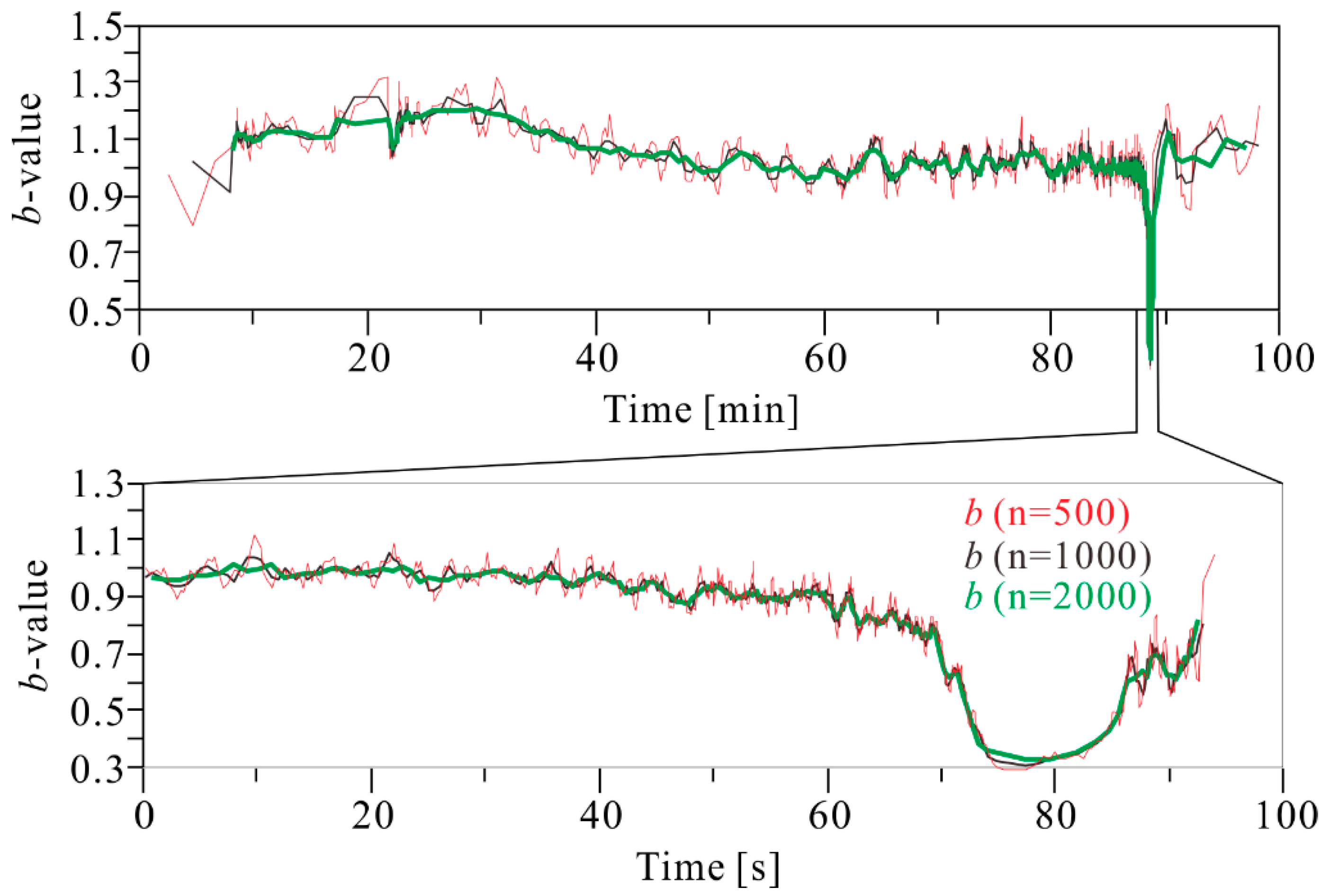Figure 2 shows b-values vs. time for n = 500, 1000, and 2000. It is clearly demonstrated that a larger n results in a smoother b-value curve, whereas a smaller n results in a higher resolution of b-value evolution. As shown in Figure 2, the results for n = 2000 were sufficiently smooth while maintaining the most basic characteristics of b-value evolution, and thus, they were used in the present study.

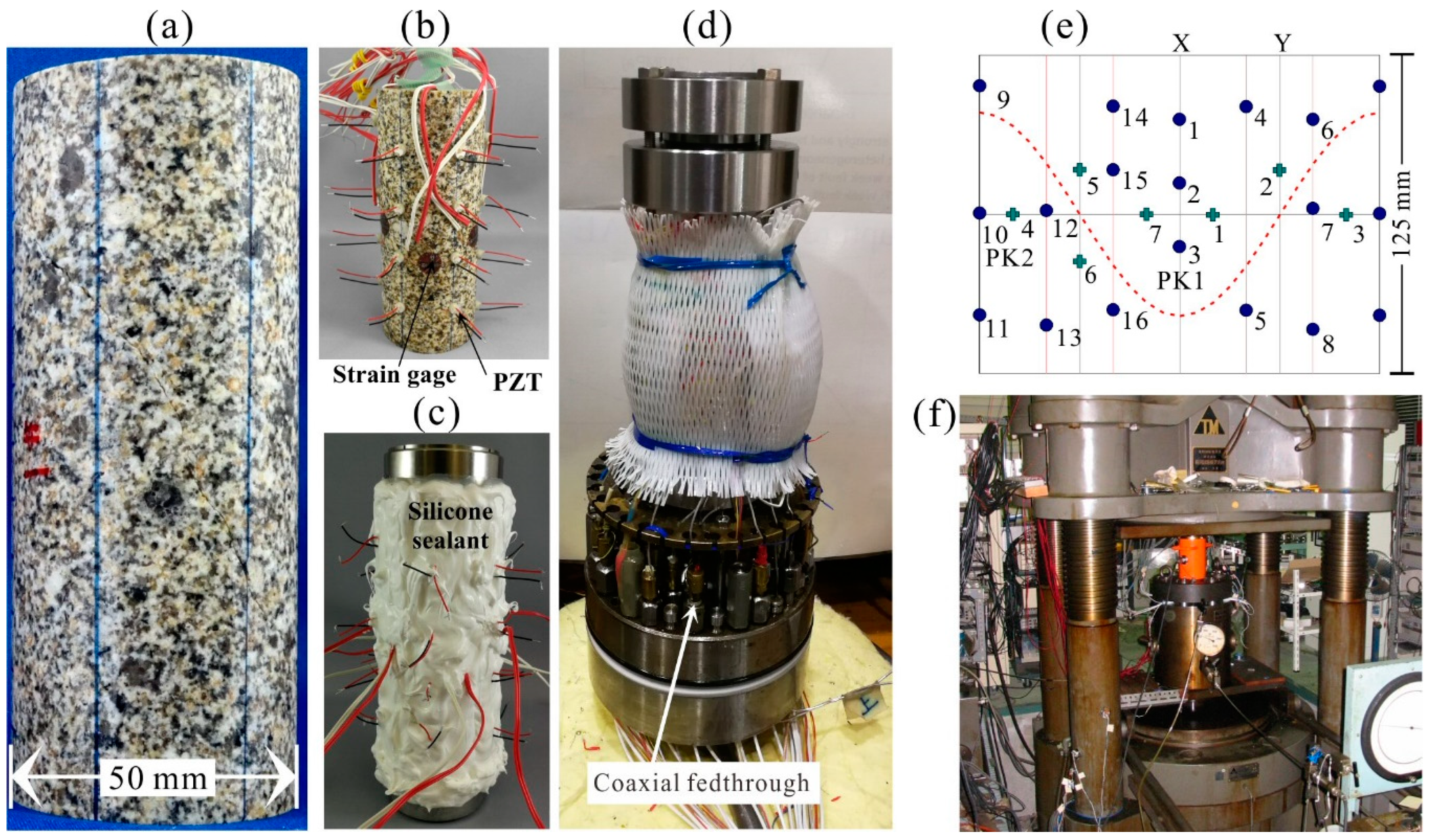
Waveform data were used for hypocenter determination. First, the method used for the automatic measurement of the arrival times of seismic signals [24] was used in the pickup of P-wave 1st motion for AE. Acoustic emission hypocenters were determined automatically using the first arrival time data of P-waves. Time-varied mean anisotropic velocities averaged from measured P-wave velocities (Vp) along multiple paths were used in hypocenter determination. For an event, clear first motions from at least four sensors were required for estimating four unknown parameters (three for source location and one for the original time). Due to heterogeneities in velocity structure and uncertainty in arrival times, more sensors generally resulted in better precision. In the present study, AE hypocenters determined by at least eight P-wave arrival times were used. The estimated location error was less than 2 mm for most hypocenters.

In order to examine the fractal behaviors of AE hypocenters, the correlation integral function was used for the estimation of multi-fractal dimensions [25]:

$$C_q(r)=\frac{1}{n}{\left[{\displaystyle \sum _{j=1}^n{\left(\frac{n_j(R\le r)}{n-1}\right)}^{q-1}}\right]}^{1/(q-1)}(q=-\infty ,\dots ,-1,0,1,\dots ,\infty )$$

(3)

where n_j (R < r) is the number of hypocenter pairs separated by a distance R less than or equal to r, q is an integer, and n is the total number of AE events analyzed. The AE hypocenter distribution generally exhibits a power law for any q, $C_q(r)\propto r^{D_q}$, and D_q defines the fractal dimension. The present study focused on D₂, which coincides with the correlation dimension.

Spatial correlation length (SCL) was also used to characterize the spatial distribution of AE hypocenters, which does not require a power-law distribution. Single-link cluster analysis was used to calculate the SCL of a set of n consecutive events [26]. First, each individual hypocenter is linked with its nearest neighbor hypocenter to form a set of clusters. Then, every cluster is linked with its nearest cluster. By repeating this process, n events are connected with n-1 links. The SCL was defined as the median of the length distribution of the n-1 links [27,28]. In order to reduce the dependence of SCL on the event number and sample dimension, a dimensionless value was given by

$${\xi }_R\left(t\right)=\raisebox{1ex}{$\xi \left(t\right)$}\!\left/ \!\raisebox{-1ex}{$l_R$}\right.$$

(4.1)

$$l_R=\raisebox{1ex}{$l_{\Omega }$}\!\left/ \!\raisebox{-1ex}{$n^{1/3}$}\right.$$

(4.2)

where t, ξ, and ξ_R are time, correlation length, and normalized correlation length, respectively, and $l_{\Omega }$ (= 50 mm) is the characteristic linear dimension of the rock specimen. The fractal dimension and SCL were estimated for a different running window, which contains 1000 hypocenters (determined by at least eight P-wave arrival times) and shifts forward by one quarter of the window length.

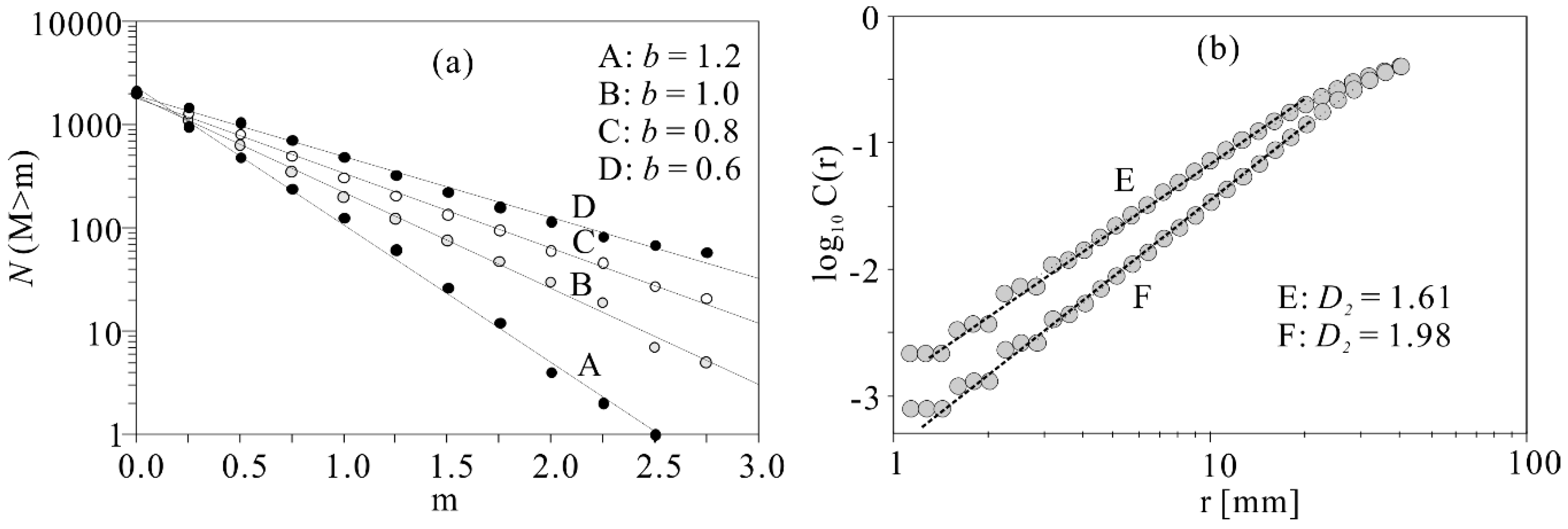
Since b-value and fractal dimension are the most important data in the present study, the quality of these data was carefully checked. Figure 3 shows examples of frequency-magnitude distribution and correlation integral functions for selected data points of typical b-values (1.2, 1.0, 0.8, and 0.6) and fractal dimensions (1.61 and 1.98). The linearity in each set was good enough for estimating reliable b-values and fractal dimensions. Note that, for examining the correlation among b-value, D₂, and SCL, b-values were calculated using the same windows for D₂ and SCL.

4. Results

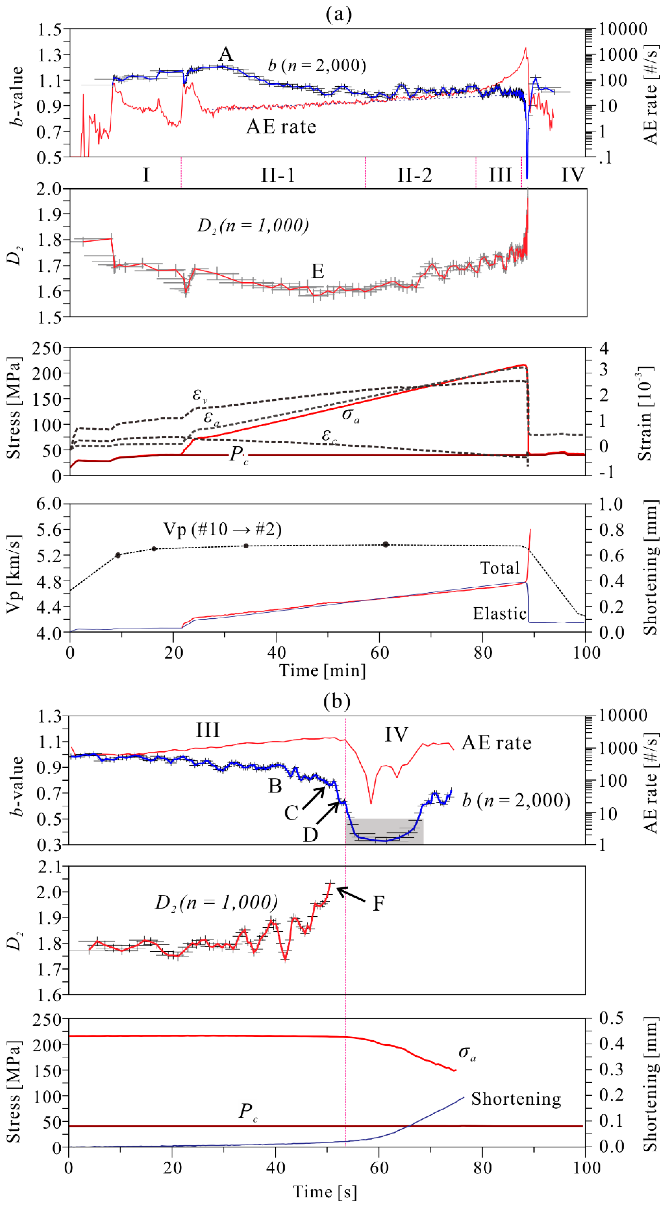
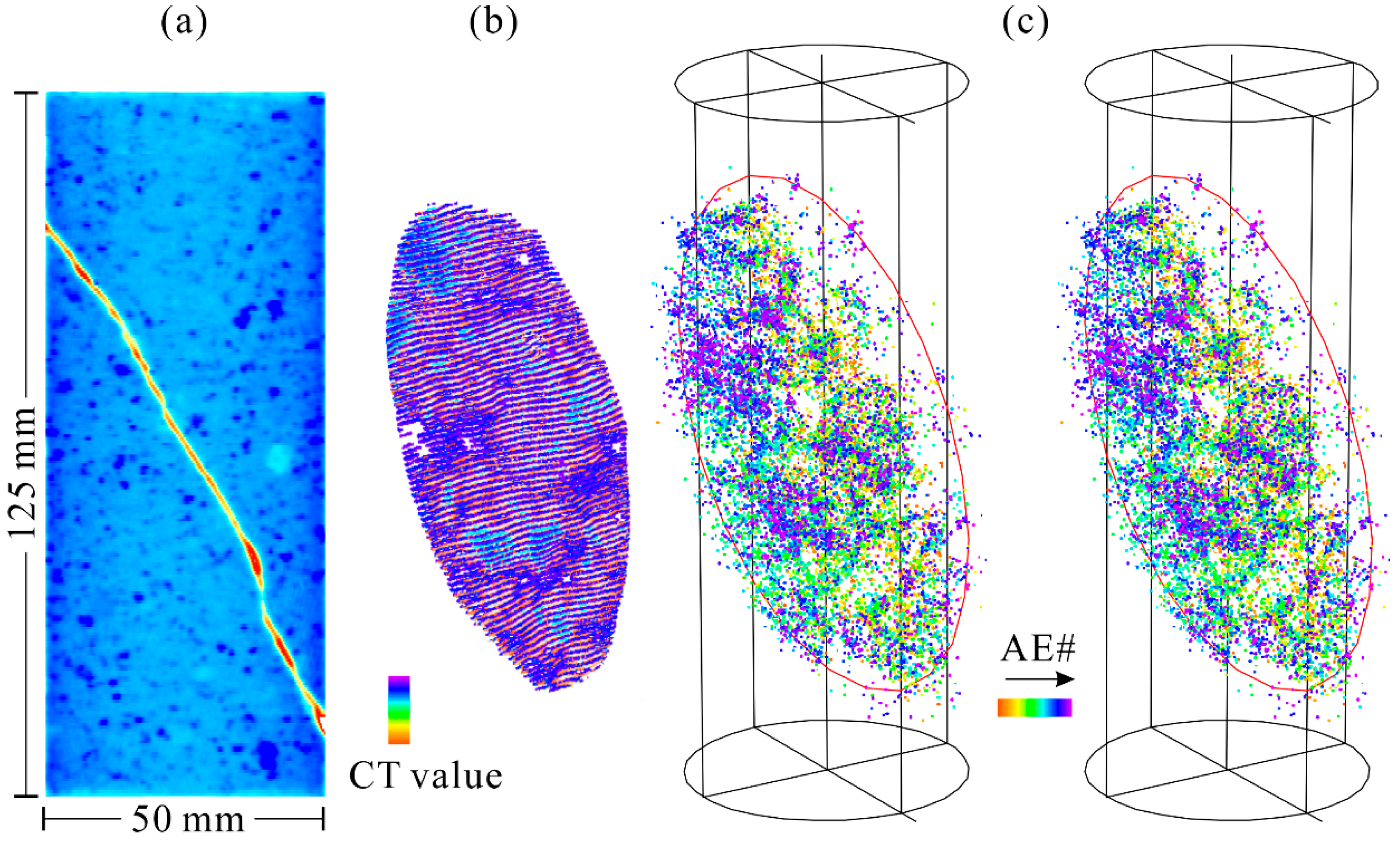
Figure 4 shows key parameters as functions of time and a zoomed view of the final two stages. Figure 5 shows a section image of the three-dimensional (3D) X-ray computed tomography (CT) scan performed after the test, the 3D fracture surface, and stereo plots of well-determined AE hypocenters determined by at least 12 arrival times for each event. The CT images showed that the involved fracture had a rough surface. Acoustic emission hypocenters were clustered on the fracture surface within a narrow offset depth.

As shown in Figure 4, AE activity was initiated at a very low stress level. Many events were observed during the hydrostatic loading stage. Such features were different for similar intact rocks, in which AE activity was initiated at a stress level approximately 60% of the strength [20]. Thus, the pre-existing immature fault exhibited a very low stress threshold for producing AE activity. In total, more than 100,000 AE events were detected by the peak detectors. A total of 64,100 events were recorded with waveforms, and 42,900 events were located by at least eight arrival times. The evolutions of AE rate, b-value, and fractal dimension of AE activity, together with rock deformation, demonstrated three pre-failure phases or stages, referred to hereinafter as stages I, II, and III, and a dynamic-aftershock stage, i.e., stage IV. The second stage can be further divided into two substages, stages II-1 and II-2. 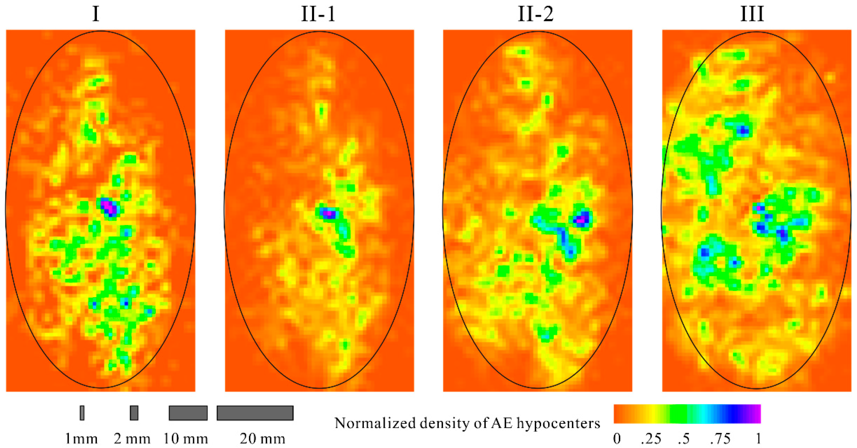Figure 6 shows normalized density maps of AE hypocenters (determined by at least 12 arrival times) on the fault surface for the pre-failure phases, stages I, II-1, II-2, and III.

Stage I was the hydrostatic compression stage, in which confining pressure and axial stress were simultaneously increased to 40 MPa. During stage I, P velocity increased from 4.5 km/s to 5.4 km/s (Figure 4a), indicating closure of major microcracks in both the fracture zone and the host rock volume. The fractal dimension decreased from approximately 1.8 to approximately 1.7, while b-value increased slightly from 1.1 to 1.2. Acoustic emission hypocenters were concentrated in many small clusters having sizes of 2 to 4 mm, which is comparable to major grain sizes (Figure 5 and Figure 6). Acoustic emission clusters were distributed along the entire domain of the fault surface, but edge areas showed a relatively low density (Figure 6).

Stage II-1, which corresponds to an axial loading to a stress level of approximately 50% strength, was characterized by (1) a gradually decreasing b-value from the maximum value of 1.2 to approximately 1.0; (2) a decreasing fractal dimension from 1.7 to 1.6; (3) an approximately constant Vp; and (4) averaged axial and volumetric strains showing elastic deformation without detectable fault slip. During stage II-2, inelastic deformation was initiated and increased slowly, and b-value fluctuated slightly with a mean value of 1.0. In addition, the fractal dimension began to increase. In stage II, the AE event rate exponentially increased with time (or axial stress). In stage II-1, fewer clusters in the center area exhibited higher density (Figure 6). During stage II-2, the number of clusters having higher density increased (Figure 6).

The nonlinear behavior of the AE rate and dilatancy deformation were the most important features of stage III (Figure 3). Acoustic emission that occurs progressively with increasing energy release can be modeled by a power law of time to failure [19]. The seismic b-value fluctuated around 1.0, with a slowly decreasing tendency, and then decreased rapidly to approximately 0.6 just before failure. Fractal dimension increased from 1.8 to 2.0. A fractal dimension of 2.0 reflects a homogeneously random distribution on the 2D plane. Together with the density distribution of AE hypocenters on the fault plane (Figure 6), it was evident that uncorrelated fracture of small asperities led to the formation of a large heterogeneous pattern. During stage III, the fault slipped by approximately 0.02 mm, which can probably be considered to be the critical slip distance.

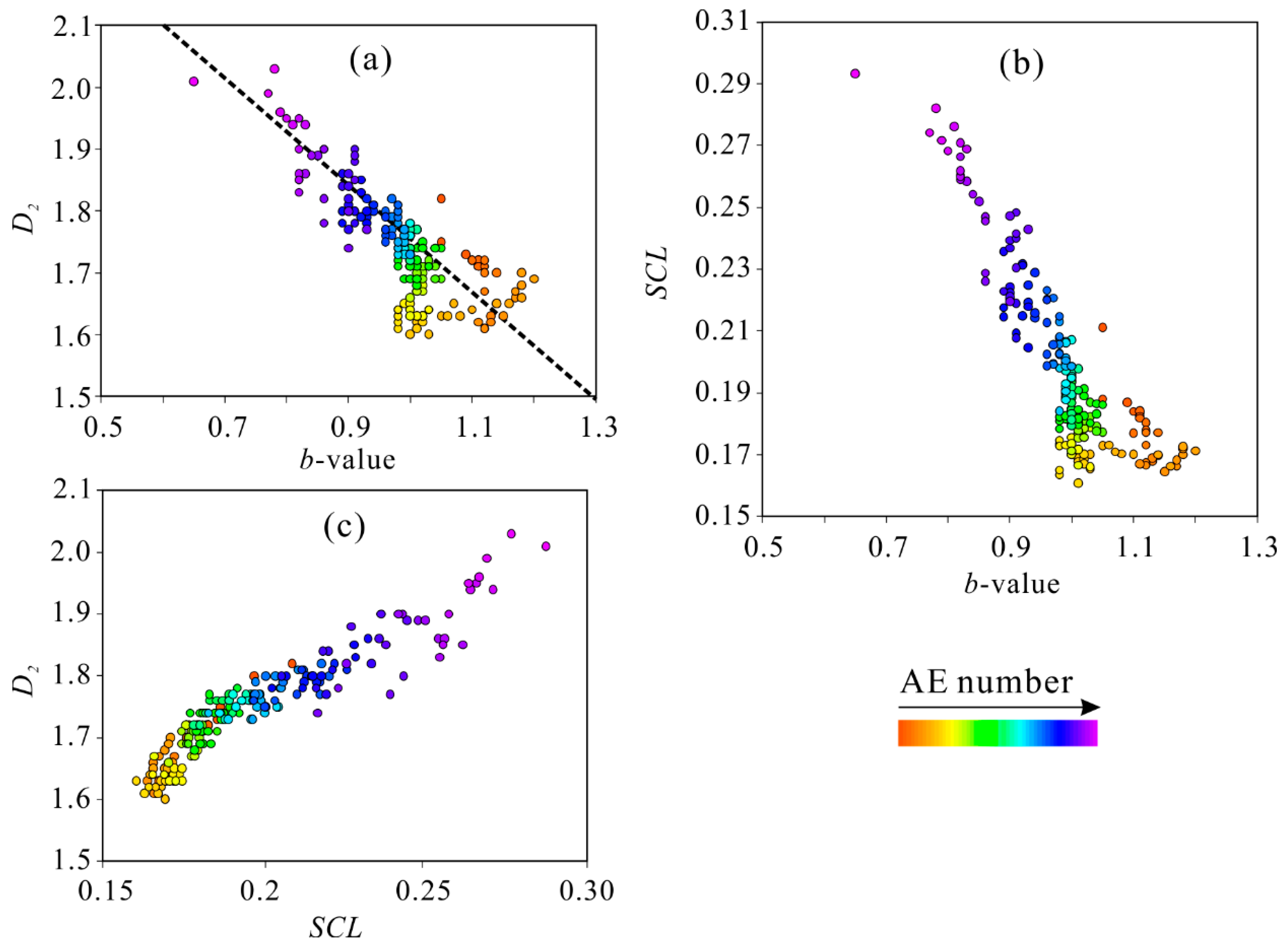
Thus far, the results of SCL have not been mentioned, because SCL behaves similarly to the fractal dimension. Our data set showed that, overall, SCL was positively correlated with the fractal dimension (Figure 7c), whereas the seismic b-value was inversely correlated with the fractal dimension and SCL (Figure 7a,b). As a result, the fractal dimension and SCL can be used alternatively.

The final pre-failure stage was followed by stage IV, including a dynamic rupture stage and following slip stages. During the dynamic stage, the axial stress dropped quickly and fault slip was accelerated. The onboard memory of the waveform recorder was fully used by the end of stage III. Thus, AE hypocenters during stage IV were not determined. Since the event rate was too high and AE signals were seriously overlapped, the obtained b-values were also less accurate.

5. Discussion and Conclusions

Early studies showed that AE activity prior to catastrophic failures in several common rock types is generally characterized by (1) increasing event rate and accelerated energy release, (2) a decrease with a subsequent precursory increase in fractal dimension and SCL, and (3) a decrease in b-value from approximately 1.5 to 0.5 for hard intact rocks and from approximately 1.1 to 0.8 for soft rocks, such as S–C cataclasite [19]. Our results for the immature fault in granite demonstrated similar patterns. However, the b-value ranged between approximately 1.2 and 0.5.

The b-value of the magnitude-frequency distribution is normally used in seismic hazard assessment for predicting the maximum magnitude. Note that (1) b-value changes with stress and (2) the maximum earthquakes are sometimes outliers of the power law governing the population behavior of a seismic sequence [3,9,19,29]. Therefore, the maximum magnitude of a given site should be determined based on the size of reactivated faults. The present experimental results showed that AE hypocenters clustered on the entire fault surface at the very early stages under a very low stress level. This suggests that the dimension of immature faults with active induced seismicity can be determined based on hypocenter distributions of seismicity that occurred in earlier stages. Planarly distributed hypocenters can be used to estimate the lower bound of fault size. It is reasonable to suggest that such a clue depends on the maturity of the faults involved. In the present study, the fault in the granite specimen was very young and had no slip history. For faults of different maturities, the stress level for the onset of detectable AE/microseismic activity and the start points of b-value and fractal dimension could be different. This is an area that should be investigated further. At a given site, there may be immature faults in the sediment and mature faults in the basement, as is the case for some sites in Ohio [7]. In seismic hazard assessment for injection-induced seismicity, we must pay more attention to immature faults because shear fracturing of such faults contributes a high level of injection-induced seismicity and greater ground motion [8]. Unfortunately, however, immature faults with less slip are difficult to detect by geophysical methods. Detailed monitoring and real-time analysis during injection are thus important for detecting unknown faults. For a specific site, in which out-zone seismicity was observed or expected, the maximum magnitude of potential inducing earthquakes should be estimated based on fault size rather than injection volume [2,3].

In conclusion, the author investigated the seismic b-value and fractal dimension for AE events during shear rupture of a pre-existing immature fault in a granite specimen under triaxial compression conditions (confining pressure: 40 MPa). The naturally-created fault had an angle of 32° with the axial stress and thus is referred to as favorably oriented.

Acoustic emission activity was initiated at a very low stress level, and the start points of b-value and fractal dimension were approximately 1.2 and 1.8, respectively. The obtained b-values decreased from approximately 1.2 to 1.0 as the shear stress increased and then quickly dropped to approximately 0.5 prior to failure. Acoustic emission hypocenters were clustered on the entire fracture surface area. With increasing stress until failure, fractal dimension exhibited the following pattern: an initial decrease from approximately 1.8 to 1.6, followed by an increase to approximately 1.8, and finally a quick increase to approximately 2.0.

Our results for b-value with respect to magnitude-frequency distribution and the fractal dimension of AE hypocenters preceding the dynamic fracturing of the immature fault demonstrated that it is possible to detect some earlier signs of fault reactivation. A gradually decreasing b-value and slowly growing fractal dimension or SCL may be an intermediate-term indication of fault reactivation, whereas a precursory rapid decrease in b-value and a rapid increase in SCL may facilitate short-term prediction of the rupture of large patches, leading to large earthquakes.

References

1. Majer, E.L.; Peterson, J.E. The impact of injection on seismicity at The Geysers, California Geothermal Field. Int. J. Rock Mech. Min. Sci. 2007, 44, 1079–1090. [Google Scholar] [CrossRef] [Green Version]
2. Lei, X.; Huang, D.; Su, J.; Jiang, G.; Wang, X.; Wang, H.; Guo, X.; Fu, H. Fault reactivation and earthquakes with magnitudes of up to Mw4. 7 induced by shale-gas hydraulic fracturing in Sichuan Basin, China. Sci. Rep. 2017, 7. [Google Scholar] [CrossRef] [PubMed]
3. Lee, K.-K.; Ellsworth, W.L.; Giardini, D.; Townend, J.; Ge, S.; Shimamoto, T.; Yeo, I.-W.; Kang, T.-S.; Rhie, J.; Sheen, D.-H. Managing injection-induced seismic risks. Science 2019, 364, 730–732. [Google Scholar] [CrossRef] [PubMed]
4. Norbeck, J.; Rubinstein, J. Hydromechanical earthquake nucleation model forecasts onset, peak, and falling rates of induced seismicity in Oklahoma and Kansas. Geophys. Res. Lett. 2018, 45, 2963–2975. [Google Scholar] [CrossRef]
5. Kwiatek, G.; Saarno, T.; Ader, T.; Bluemle, F.; Bohnhoff, M.; Chendorain, M.; Dresen, G.; Heikkinen, P.; Kukkonen, I.; Leary, P. Controlling fluid-induced seismicity during a 6.1-km-deep geothermal stimulation in Finland. Sci. Adv. 2019, 5. [Google Scholar] [CrossRef] [PubMed]
6. Lei, X.; Wang, Z.; Su, J. The December 2018 ML 5.7 and January 2019 ML 5.3 Earthquakes in South Sichuan Basin Induced by Shale Gas Hydraulic Fracturing. Seismol. Res. Lett. 2019, 90. [Google Scholar] [CrossRef]
7. Kozłowska, M.; Brudzinski, M.R.; Friberg, P.; Skoumal, R.J.; Baxter, N.D.; Currie, B.S. Maturity of nearby faults influences seismic hazard from hydraulic fracturing. Proc. Natl. Acad. Sci. USA 2018, 115, E1720–E1729. [Google Scholar] [CrossRef] [PubMed]
8. Radiguet, M.; Cotton, F.; Manighetti, I.; Campillo, M.; Douglas, J. Dependency of near-field ground motions on the structural maturity of the ruptured faults. Bull. Seismol. Soc. Am. 2009, 99, 2572–2581. [Google Scholar] [CrossRef]
9. Lei, X. Dragon-Kings in rock fracturing: Insights gained from rock fracture tests in the laboratory. Eur. Phys. J. Spec. Top. 2012, 205, 217–230. [Google Scholar] [CrossRef]
10. Mogi, K. Study of elastic shocks caused by the fracture of heterogeneous materials and its relations to earthquake phenomena. Bull. Earthq. Res. Inst. Tokyo Univ. 1962, 40, 125–173. [Google Scholar]
11. Lockner, D.A.; Byerlee, J.D.; Kuksenko, V.; Ponomarev, A.; Sidorin, A. Quasi-static fault growth and shear fracture energy in granite. Nature 1991, 350, 39–42. [Google Scholar] [CrossRef]
12. Lei, X. Typical phases of pre-failure damage in granitic rocks under differential compression. Geol. Soc. Lond. Spec. Publ. 2006, 261, 11–29. [Google Scholar] [CrossRef] [Green Version]
13. Meredith, P.G.; Main, I.G.; Jones, C. Temporal variations in seismicity during quasi-static and dynamic rock failure. Tectonophysics 1990, 175, 249–268. [Google Scholar] [CrossRef]
14. Moura, A.; Lei, X.; Nishisawa, O. Self-similarity in rock cracking and related complex critical exponents. J. Mech. Phys. Solids 2006, 54, 2544–2553. [Google Scholar] [CrossRef]
15. Main, I.G.; Meredith, P.G.; Sammonds, P.R. Temporal variations in seismic event rate and b-values from stress corrosion constitutive laws. Tectonophysics 1992, 211, 233–246. [Google Scholar] [CrossRef]
16. Goebel, T.; Schorlemmer, D.; Becker, T.; Dresen, G.; Sammis, C. Acoustic emissions document stress changes over many seismic cycles in stick-slip experiments. Geophys. Res. Lett. 2013, 40, 2049–2054. [Google Scholar] [CrossRef] [Green Version]
17. Rivière, J.; Lv, Z.; Johnson, P.; Marone, C. Evolution of b-value during the seismic cycle: Insights from laboratory experiments on simulated faults. Earth Planet. Sci. Lett. 2018, 482, 407–413. [Google Scholar] [CrossRef]
18. Lei, X.; Li, S.; Liu, L. Seismic b-Value for Foreshock AE Events Preceding Repeated Stick-Slips of Pre-Cut Faults in Granite. Appl. Sci. 2018, 8, 2361. [Google Scholar] [CrossRef]
19. Lei, X.; Satoh, T. Indicators of critical point behavior prior to rock failure inferred from pre-failure damage. Tectonophysics 2007, 431, 97–111. [Google Scholar] [CrossRef]
20. Lei, X.; Kusunose, K.; Nishizawa, O.; Cho, A.; Satoh, T. On the spatio-temporal distribution of acoustic emissions in two granitic rocks under triaxial compression: The role of pre-existing cracks. Geophys. Res. Lett. 2000, 27, 1997–2000. [Google Scholar] [CrossRef] [Green Version]
21. Lei, X. How do asperities fracture? An experimental study of unbroken asperities. Earth Planet. Sci. Lett. 2003, 213, 347–359. [Google Scholar] [CrossRef]
22. Gutenberg, B.; Richter, C.F. Frequency of earthquakes in California. Bull. Seismol. Soc. Am. 1944, 34, 185–188. [Google Scholar]
23. Colombo, I.S.; Main, I.; Forde, M. Assessing damage of reinforced concrete beam using “b-value” analysis of acoustic emission signals. J. Mater. Civ. Eng. 2003, 15, 280–286. [Google Scholar] [CrossRef]
24. Yokota, T.; Zhou, S.; Mizoue, M.; Nakamura, I. An automatic-measurement of arrival-time of seismic-waves and its application to an online processing system. Bull. Earthq. Res. Inst. Univ. Tokyo 1981, 56, 449–484. [Google Scholar]
25. Kurths, J.; Herzel, H. An attractor in a solar time series. Phys. D Nonlinear Phenom. 1987, 25, 165–172. [Google Scholar] [CrossRef]
26. Frohlich, C.; Davis, S.D. Single-link cluster analysis as a method to evaluate spatial and temporal properties of earthquake catalogues. Geophys. J. Int. 1990, 100, 19–32. [Google Scholar] [CrossRef]
27. Tyupkin, Y.S.; Di Giovambattista, R. Correlation length as an indicator of critical point behavior prior to a large earthquake. Earth Planet. Sci. Lett. 2005, 230, 85–96. [Google Scholar] [CrossRef]
28. Zöller, G.; Hainzl, S.; Kurths, J. Observation of growing correlation length as an indicator for critical point behavior prior to large earthquakes. J. Geophys. Res. 2001, 106, 2167. [Google Scholar] [CrossRef]
29. Yoon, C.E.; Huang, Y.; Ellsworth, W.L.; Beroza, G.C. Seismicity during the initial stages of the Guy-Greenbrier, Arkansas, earthquake sequence. J. Geophys. Res. Solid Earth 2017, 122, 9253–9274. [Google Scholar] [CrossRef]
Figure 1. (a) Photograph of the test specimen. (b) Specimen with piezoelectric transducers (PZT) and cross-type strain gauges mounted. (c) Specimen and endpieces covered with silicone sealant. (d) Specimen-cover assembly. (e) Plot showing the distributions of PZTs (solid circles) and cross-type strain gauges (crosses). (f) Photograph of the load frame used in the test. The maximum amplitudes of AE signals from PK1 and PK2 were recorded by two peak detectors and were used for the calculation of seismic b-value.
Applsci 09 02498 g001
Figure 2. Seismic b-value estimated using the maximum likelihood method for a running window of n events with a step of n/4 events.
Applsci 09 02498 g002
Figure 3. Examples of (a) frequency-magnitude distribution and (b) and correlation function for selected data points A–F.
Applsci 09 02498 g003
Figure 4. Plots show (a) key parameters with respect to time and (b) close-up plots of the final two stages. Acoustic emission rates were calculated for every 10 s. The b-values were estimated using the maximum likelihood method for a running window of n = 2000 events with a step of 500 events. The fractal dimension (D2) was estimated for a running window and a step of n = 1000 and 500 hypocenters. Axial, circumferential, and volumetric strains (εa, εc, and εv) were obtained as the average of data recorded by seven pairs of stain gauges adhered directly to the surface of the specimen. The axial shortening of the specimen was estimated based on piston displacement and was calibrated using the elastic portion of the mean axial strain, εa. The shaded period in (b) corresponds to the dynamic rupture stage, in which AE occurred at a very high rate and several events could not be separated, and thus the estimated b-values were inaccurate.
Applsci 09 02498 g004
Figure 5. (a) Vertical section of three-dimensional X-ray computed tomography (CT) scan performed after the experiment. The fracture zone is characterized by very low CT value. (b) Three-dimensional fracture surface. (c) Stereo plots of well-determined (by at least 12 P arrival times) AE hypocenters. Hypocenter dots are colored according to event number.
Applsci 09 02498 g005
Figure 6. Normalized density distribution of AE hypocenters on the fault plane for the pre-failure phases (stages I, II-1, II-2, and III, as indicated in Figure 4).
Applsci 09 02498 g006
Figure 7. Plots showing correlations between b-value and fractal dimension (a), b-value and SCL (b), and SCL and fractal dimension (c). The data circles are colored according to AE number to show the temporal evolution path.
Applsci 09 02498 g007