Dynamic Path Planning via Enhanced ACO and DWA Algorithms

Abstract

Path planning for autonomous mobile robots in dynamic environments is a critical challenge, particularly when robots must navigate both known and unknown obstacles in real-time. Traditional methods like ant colony optimization (ACO) have shown promise in global path planning but often suffer from slow convergence and the risk of getting trapped in local optima. Similarly, while the dynamic window approach (DWA) excels in real-time obstacle avoidance, it exhibits delayed response and higher failure rates in scenarios with fast-moving obstacles. To address these challenges, this study proposes a hybrid path planning framework, IACO-QDWA, which integrates an improved ACO (IACO) for global path optimization with a Q-learning-enhanced DWA (QDWA) for dynamic obstacle avoidance. IACO improves global path search through goal-oriented initialization and adaptive pheromone updates, while QDWA enhances local decision-making by optimizing the state-action space. The experiments demonstrate that IACO-QDWA achieves a reasonable balance between path quality, obstacle avoidance success rate, and real-time performance. It exhibits stable obstacle avoidance behavior and reliable navigation capabilities in highly dynamic environments.

1. Introduction

With the continuous advancement of robotic technologies, mobile robots have become increasingly prevalent across a wide range of application domains [1]. As a core element of autonomous navigation, the performance of path planning algorithms has emerged as a critical indicator for assessing the intelligence level and environmental adaptability of mobile robots [2]. A central challenge in mobile robot path planning lies in generating an optimal and collision-free trajectory from a known starting point to a designated target point in a fast and reliable manner [3].

In general, path planning methods can be categorized into global and local approaches. Global path planning aims to compute an optimal path within a fully known map, with existing solutions spanning traditional algorithms [4,5] and a variety of intelligent optimization techniques, such as ant colony optimization (ACO) [6], genetic algorithms [7,8], particle swarm optimization (PSO) [9], rapidly exploring random trees (RRT) [10], and reinforcement learning [11]. Local path planning, by contrast, relies on real-time sensor data to perceive unknown or dynamic obstacles and ensure online obstacle avoidance. Representative methods include the dynamic window approach (DWA) [12] and artificial potential field (APF) methods [13].

While global path planning provides a complete route based on known maps and offers strong overall optimality, it often suffers from high computational costs in complex environments and poor adaptability to dynamic or partially unknown conditions [14]. Furthermore, the paths generated may lack smoothness, limiting their practical applicability [15,16]. To overcome these challenges, numerous enhancement strategies have been proposed. For instance, reference [17] innovatively integrates a Q-evaluation mechanism into ACO for more effective node selection. This enhancement improves the reliability of path evaluation and accelerates convergence, addressing ACO’s issues with slow convergence and sensitivity to parameters. Reference [18] introduces a genetically augmented exploration mechanism, objective-guided optimization, and a dual restart strategy, significantly enhancing path smoothness and global search performance. In [19], PSO is enhanced by employing a bi-population structure and a random perturbation strategy, effectively improving search diversity and avoiding premature convergence and local optima. In [20], an improved kinematically constrained bi-directional RRT algorithm is proposed that improves guidance, ensures kinematically feasible sampling, and smooths dual-tree connections, enabling safer, smoother, and more efficient robot paths with significant reductions in path length and planning time. Reference [21] proposes a dual-mode, learning-based path planning framework, integrating global guidance and local reinforcement learning. This approach reduces congestion and significantly improves system throughput and efficiency compared to existing methods.

On the other hand, local path planning provides real-time responsiveness and adaptability to dynamic environments, but its reliance on local information often results in local optima and suboptimal efficiency [22,23]. To address this issue, reference [24] proposes a hybrid algorithm, combining modified golden jackal optimization and DWA, which improves global search efficiency through diverse search strategies and a vulture-inspired guiding mechanism, while enhancing obstacle avoidance by optimizing the obstacle evaluation function. Experimental results show a reduction in path length by 10.76–25.46% and a decrease in local optima occurrences from 6 to 2. In reference [25], an improved APF method is integrated with an enhanced deep deterministic policy gradient framework to boost path planning safety and training efficiency, using strategy switching and obstacle detection to achieve safer navigation and faster convergence.

However, despite these advances in both global and local planning, many existing improvements still optimize either global planning or local avoidance, making it difficult to simultaneously achieve high global path quality and robust real-time performance in complex dynamic environments. In this work, we adopt ACO as the global planner due to its effective discrete-map exploration capability, and choose DWA for local planning as it naturally satisfies kinematic constraints and supports real-time trajectory evaluation. To enhance adaptability to fast-moving obstacles without introducing heavy training costs, Q-learning is integrated into DWA, enabling lightweight online policy adjustment. Based on these considerations, we propose the IACO–QDWA framework, which combines an improved ACO (IACO) for faster convergence and reduced local stagnation with a Q-learning-enhanced DWA (QDWA) for more stable dynamic obstacle avoidance.

2. Principles and Improvements of Ant Colony Optimization Algorithm

The ACO algorithm is inspired by the collective foraging behavior of ants, where pheromones are deposited on paths between food sources and nests to guide subsequent search. Paths with higher pheromone concentration are more likely to be selected, as they typically correspond to shorter or more favorable routes. As the iterations proceed, an increasing number of ants are attracted to paths with higher pheromone intensity, leading to convergence toward an optimal solution.

When ants encounter multiple available paths, the next path is selected using the roulette wheel method. The corresponding probability is defined by Equation (1):

$$P_{ij}^k=\left\{\begin{array}{cc}\hfill {\displaystyle \frac{{\tau }_{ij}^{\alpha }(t)\cdot {\eta }_{ij}^{\beta }(t)}{{\displaystyle {\sum }_{j\in allowe{d}_k}{\tau }_{ij}^{\alpha }(t)\cdot {\eta }_{ij}^{\beta }(t)}}}\hfill & , j\in allowe{d}_k\hfill \\ \hfill 0\hfill & , else\hfill \end{array}\right.$$

(1)

where $i,j$ represent the starting and ending points of a path in the grid map, $k$ denotes the index of the ant, $allowe{d}_k$ is the set of paths available for ant $k$ to choose from, $\alpha$ is the pheromone influence factor, $\beta$ is the heuristic information factor, ${\tau }_{ij}(t)$ is the pheromone concentration from $i$ to $j$ at iteration $t$, and ${\eta }_{ij}(t)$ is the heuristic information from $i$ to $j$ at iteration $t$, representing the visibility of the ant from $i$ to $j$ (see Table A1). The heuristic function is defined in Equation (2):

$${\eta }_{ij}^{\beta }(t)=1/d_{ij}$$

(2)

where $d_{ij}$ is the Euclidean distance between the two points.

After one iteration of ACO, the pheromone concentration on different paths is updated. The pheromone update rule is given by Equation (3), where the pheromone increment $∆{\tau }_{ij}$ is defined in Equation (4).

$${\tau }_{ij}(t+1)={\tau }_{ij}(t)\cdot (1-\rho )+∆{\tau }_{ij},0<\rho <1$$

(3)

where $\rho$ is the pheromone evaporation rate.

$$∆{\tau }_{ij}={\displaystyle \sum _{k=1}^m∆{\tau }_{ij}^k}$$

(4)

where $∆{\tau }_{ij}^k$ is the pheromone deposited by the $k$ ant on the path from $i$ to $j$.

2.1. Improved Ant Colony Optimization Algorithm

The improvement strategies adopted in the proposed IACO are designed to address the main shortcomings of the traditional ACO in robot path planning, including slow convergence, premature stagnation, and the generation of redundant path nodes. Instead of introducing additional hybrid optimization operators or external guidance frameworks, this study focuses on enhancing the internal guidance and adaptability of the pheromone-based search process. Accordingly, targeted improvements are implemented at the stages of initialization, pheromone updating, parameter adaptation, and path post-processing, as detailed in Section 2.1.1, Section 2.1.2, Section 2.1.3 and Section 2.1.4. For clarity, the term traditional ACO refers to the standard ant colony optimization described by Equations (1)–(4), while IACO denotes the improved version proposed in this study.

Although each improvement addresses a specific limitation of the traditional ACO, they are designed to operate cooperatively rather than independently. The goal-oriented initialization provides effective early-stage guidance, which is subsequently reinforced by the adaptive pheromone update during the iterative search process. Meanwhile, the dynamic adjustment of the pheromone and heuristic factors regulates the balance between exploration and exploitation across different search phases, thereby preventing premature stagnation. Finally, the node pruning strategy acts as a post-processing step to refine the optimized path without interfering with the global search process.

2.1.1. Optimization of the Initialization Process

In the initialization phase of the ACO algorithm, a uniform pheromone distribution reduces the efficiency of early path planning. To address this issue, a goal-oriented initialization mechanism is introduced, which incorporates information about the start and end points to provide more effective guidance during the early search stage. The goal-oriented initial pheromone concentration is calculated using Equation (5):

$${\tau }_{ij}(0)=\left\{\begin{array}{cc}\hfill {\displaystyle \frac{d_{ab}}{L_{ai}+d_{ij}+d_{jb}}}\hfill & , j\in allowe{d}_k\hfill \\ \hfill 0\hfill & , else\hfill \end{array}\right.$$

(5)

where $d_{ab}$ is the Euclidean distance between the start point $a$ and the end point $b$, and $L_{ai}$ is the path length traveled by the ant from the start point $a$ to path point $i$.

2.1.2. Adaptive Pheromone Update Strategy

In the ACO algorithm, the update of pheromone concentration relies on the random exploration of the ant colony. Although this mechanism is simple, it lacks efficiency and effective guidance, making the algorithm prone to converging to local optima. To address this limitation, an adaptive pheromone update strategy based on positive and negative feedback is introduced. This strategy uses the average path length of the current iteration as a reference for pheromone adjustment: when the path length is shorter than the average, the pheromone concentration on the corresponding path is increased; conversely, when the path length is longer, the pheromone concentration is reduced. The adaptive pheromone update strategy is defined by Equation (6):

$$∆{\tau }_{ij}^k=\left\{\begin{array}{l}{\displaystyle \frac{Q}{L_k}}+\phi \cdot {\displaystyle \frac{L_k-L_{opt}}{L_{ave}-L_{opt}}} ,L_k\le L_{ave}\\ {\displaystyle \frac{Q}{L_k}}-\phi \cdot {\displaystyle \frac{L_k-L_{opt}}{L_{ave}-L_{opt}}} ,L_k>L_{ave}\end{array}\right.$$

(6)

where $L_{opt}$ is the length of the optimal path in the current iteration, $L_{ave}$ is the average path length in the current iteration, and $\phi$ is the pheromone allocation weight factor.

2.1.3. Design of Adaptive Pheromone and Heuristic Factors

In the early stages of the ACO algorithm, path selection mainly depends on pheromone accumulation, which tends to bias the search toward suboptimal paths and may lead to premature convergence in later iterations. To mitigate this issue, an adaptive parameter adjustment strategy is proposed. In the initial phase, a higher $\alpha$ and a lower $\beta$ are adopted to encourage broader exploration. As the number of iterations increases, $\alpha$ gradually decreases, while $\beta$ correspondingly increases, thereby accelerating the convergence of the algorithm. The adaptive adjustment of parameters is calculated using Equations (7) and (8):

$$\alpha (t)=2\cdot \cos ({\displaystyle \frac{\pi \cdot t}{2\cdot t_{\max }}})+\alpha (0)$$

(7)

$$\beta (t)=2\cdot \sin ({\displaystyle \frac{\pi \cdot t}{2\cdot t_{\max }}})+\beta (0)$$

(8)

where $t$ is the current iteration number.

2.1.4. Improved Path Point Management Strategy

During the search for an optimal path, the ACO algorithm may generate redundant node information, resulting in excessively long paths. To address this issue, a path optimization strategy incorporating a greedy mechanism is proposed. First, a path node information library is constructed based on the ACO results. Starting from the initial point, the algorithm attempts to bypass nearby nodes and directly connect to farther nodes. If the resulting path is feasible, the corresponding intermediate nodes are removed; otherwise, the process returns to the nearest node and repeats the same operation, as illustrated in Figure 1.

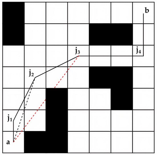
Figure 1. Schematic of redundant node removal. Black and white squares represent obstacles and traversable areas, respectively. ‘a’ and ‘b’ denote the start and target positions. j₁–j₄ are path nodes from ACO. The red dashed line shows the line-of-sight check, and black solid lines represent the optimized path.

3. Principle and Improvement of the DWA Algorithm

3.1. Principle of the DWA Algorithm

The DWA is a classic local path planning algorithm, consisting mainly of two components: the motion model and the evaluation function. The motion model is responsible for predicting the robot’s motion state over a short period in the future. The evaluation function selects the optimal trajectory from multiple predicted trajectories. The robot’s motion model is defined by Equations (9)–(11):

$$x(t+1)=x+v\cdot \cos \left(\theta \right)\cdot dt$$

(9)

$$y(t+1)=y+v\cdot \sin \left(\theta \right)\cdot dt$$

(10)

$$\theta (t+1)=\theta +\omega \cdot dt$$

(11)

where $x,y$ are the coordinates of the mobile robot; $v$ and $\omega$ represent the current linear velocity and angular velocity, respectively; and $\theta$ is the current heading angle.

In the DWA algorithm, trajectory optimization is achieved by adjusting the velocity control parameters to enable effective obstacle avoidance and path planning in dynamic environments. This process relies on precisely constraining the robot’s motion model parameters within the sampling space. The specific constraints are as follows:

1.

According to the robot’s motion state, the maximum feasible ranges of linear velocity and angular velocity can be determined as $V_S$, which is calculated using Equation (12):

$$V_S=\left\{(v,\omega )\left|\begin{array}{c}v\in [v_{\min }, v_{\max }]\\ \omega \in [{\omega }_{\min }, {\omega }_{\max }]\end{array}\right.\right\}$$

(12)

2.

Robot’s actual motion velocity, affected by the torque of its motors, is constrained to $V_d$, defined by Equation (13):

$$V_d=\left\{(v,\omega )\left|\begin{array}{c}v\in [v_0-{\alpha }_{\max }dt, v_0+{\alpha }_{\max }dt]\\ \omega \in [{\omega }_0-{\beta }_{\max }dt, {\omega }_0+{\beta }_{\max }dt]\end{array}\right.\right\}$$

(13)

3.

Here, ${\alpha }_{\max }$ is the maximum linear acceleration; $dt$ is the time step; and ${\beta }_{\max }$ is the current angular acceleration.

4.

Based on the robot’s safety requirements, the acceleration space that ensures safe obstacle avoidance is $V_a$, given by Equation (14):

$$V_a=\left\{(v,\omega )\left|\begin{array}{c}v\in \left[0, \sqrt{2\cdot dist(v,\omega )\cdot {\alpha }_{\max }}\right]\\ \omega \in \left[0, \sqrt{2\cdot dist(v,\omega )\cdot {\beta }_{\max }}\right]\end{array}\right.\right\}$$

(14)

5.

Here, $dist(v,\omega )$ is the distance from the current trajectory to the nearest obstacle.

Finally, based on the robot’s motion characteristics and the surrounding obstacles, the velocity range of the dynamic window can be defined as $V_r$, computed by Equation (15):

$$V_r=V_s\cap V_d\cap V_a$$

(15)

By sampling within the dynamic window, the generated trajectory plot is obtained as shown in Figure 2. The motion trajectory depends on processing the linear and angular velocities of each sampling point over a predefined time $t$.

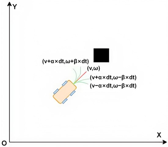
Figure 2. Trajectory generation within a dynamic window based on sampled linear and angular velocities (orange: mobile robot; black: obstacle).

After obtaining the robot’s potential motion trajectories, the evaluation function scores these predicted paths and selects the trajectory that best fits the current environment and target. The evaluation function for trajectory selection is given by Equation (16):

$$J(v,\omega )=\mu \cdot heading(v,\omega )+\eta \cdot dist(v,\omega )+\lambda \cdot vel(v,\omega )$$

(16)

where $heading(v,\omega )$ is the heading evaluation sub-function, used to calculate the directional deviation between the predicted trajectory’s end pose (position and velocity) and the target point; $vel(v,\omega )$ is the magnitude of the current trajectory’s velocity; $\mu$ is the heading weight coefficient; $\eta$ is the safety distance coefficient; and $\lambda$ is the velocity weight coefficient.

3.2. Multi-Objective DWA Algorithm Based on Reinforcement Learning

Although the evaluation function in Equation (16) enables real-time trajectory selection, its performance heavily relies on manually tuned weights, which may lead to delayed responses and local stagnation when facing fast-moving obstacles. Therefore, a lightweight Q-learning mechanism is introduced to adaptively enhance local decision-making while preserving the real-time feasibility of the DWA framework.

3.2.1. Establishing the State Space and Action Space Model

To integrate Q-learning into the DWA framework while avoiding the computational intractability of a classic Q-table in continuous high-dimensional state spaces, this work adopts a uniform discretization strategy that maps continuous state variables into a finite set of discrete states, thereby constructing a tractable tabular Q-learning system.

The state vector is designed as a five-dimensional relative representation, $S=(d_g,{\theta }_e,d_o,v,\omega )$, where $d_g$ denotes Euclidean distance from the robot to the current local goal (or the next waypoint); ${\theta }_e$ denotes heading error between the robot’s orientation and the direction toward the local goal; and $d_o$ denotes distance to the nearest obstacle. Each state variable is uniformly quantized according to the ranges and discrete intervals listed in Table 1.

Table 1. Discretization settings of state variables.

Symbol	Range	Number of Bins	Remarks
$d_g$	0–5 m	10	Local goal distance within sensing range
${\theta }_e$	−π–π rad	12	Covers full circumferential directions
$d_o$	0–4 m	8	Within the safety margin
$v$	0–2 m/s	5	Up to the robot’s maximum speed
$\omega$	−π/4–π/4 rad/s	5	Up to the robot’s maximum angular speed

The action space $A$ is defined as a set of control increments, $A=\{(∆v,∆\omega )\}$, where $∆v$ denotes the increment of linear velocity, $∆\omega$ denotes the increment of angular velocity. The increments are discretized as $∆v\in \{-0.2,0,+0.2\}$ m/s and $∆\omega \in \{-0.2,0,+0.2\}$ rad/s, aligning with the velocity resolution used in DWA sampling and the robot’s dynamic constraints. This results in a tractable Q-table with $\left|S\right|$ = 24,000 states (derived from Table 1) and $\left|A\right|$ = 9 actions.

Sensor noise and perception latency are simplified in this model; obstacle detection is assumed to be instantaneous and accurate within the robot’s sensing range. This simplification allows the research to focus on evaluating the reactive decision-making performance of Q-learning in dynamic environments and lays a foundation for future extensions under more complex perceptual conditions. Through the above discretization design, the proposed approach preserves the expressive power of the state information while avoiding the state space explosion that would occur with a continuous high-dimensional representation, thereby enabling real-time operation of tabular Q-learning in practical systems.

3.2.2. Design of the Reward Function

To guide the learning process toward safe and efficient navigation, a composite reward function $R$ is designed by jointly considering target attraction, motion stability, smoothness, and collision avoidance. The reward function consists of two components: positive rewards and negative penalties.

The purpose of the positive reward mechanism is to encourage the robot to enhance its obstacle avoidance performance, stability, and path smoothness. Specifically, it includes three types of rewards: target-approaching reward $R_1$; motion-stability reward $R_2$ (applied only when no obstacles are detected); and trajectory-optimization reward $R_3$. The reward components are calculated using Equations (17)–(19):

$$R_1=k_1\times (d_{new}-d_{old})$$

(17)

$$R_2=k_2\times (1-\left|v_{new}-v_{old}\right|)+k_t\times (1-\left|{\omega }_{new}-{\omega }_{old}\right|)$$

(18)

$$R_3=k_3\cdot e^{-\sigma (Q_{new}-Q_{old})}-k_{\mathrm{t}}\cdot ({\theta }_{\mathrm{new}}-{\theta }_{\mathrm{old}})$$

(19)

where $d_{old}$ is the distance from the robot’s current position to the target; $d_{new}$ is the distance from the robot’s new position (after executing the action) to the target; $v_{new}$ and $v_{old}$ are the linear velocities before and after the action, respectively; ${\omega }_{new}$ and ${\omega }_{old}$ are the angular velocities before and after the action; $Q_{new}$ and $Q_{old}$ represent the values of the motion state before and after the action; $\sigma$ is the sensitivity coefficient for adjusting trajectory deviation; ${\theta }_{\mathrm{new}}$ and ${\theta }_{\mathrm{old}}$ are the robot’s heading angles before and after the action; $k_1,k_2,k_3,k_t$ denotes the weight coefficient.

To prevent the robot from exhibiting potentially dangerous behaviors, a negative penalty mechanism is designed. It consists of two categories: the time-consuming turning penalty $R_4$ and the obstacle-collision penalty $R_5$. The penalty components are calculated using Equations (20) and (21):

$$R_4=-k_4\times dt-k_t\times \left|{\omega }_{new}-{\omega }_{old}\right|$$

(20)

$$R_5=-k_5\cdot e^{-(d-d_{safe})}$$

(21)

where $dt$ denotes the single-step time interval; $k_4,k_5$ is the weight coefficient; $d$ represents the distance to the obstacle; $d_{safe}$ is the safety distance, which is a constant.

The total reward function $R$ is computed by Equation (22):

$$R=R_1+R_2+R_3+R_4+R_5$$

(22)

The reward terms and their corresponding weights are designed to reflect the relative importance of safety, efficiency, and motion stability in dynamic obstacle avoidance. Specifically, obstacle-related penalties are assigned higher weights to strictly enforce collision avoidance, while target-approaching and smoothness terms are weighted to balance efficiency and trajectory quality. The weight values are initially selected based on common practices in DWA-based navigation and empirically tuned to ensure stable behavior across different scenarios. To assess robustness, we conducted preliminary tuning experiments by varying each weight within a reasonable range while keeping others fixed. The observed navigation performance exhibited consistent trends, and no abrupt degradation was found within these ranges, indicating that the proposed reward formulation is not overly sensitive to precise weight values. Therefore, the selected weights provide a practical and stable balance among multiple navigation objectives.

3.2.3. Q-Learning Update Mechanism

During the process of searching for the optimal path, the robot interacts with the environment and updates its Q-value table based on the immediate feedback it receives. The Q-learning update mechanism is defined by Equation (23):

$$Q^{\prime }(S,A)=Q(S,A)+\lambda \times (R+\gamma \times {\max }_{a^{\prime }}Q(S^{\prime },A^{\prime })-Q(S,A))$$

(23)

where $Q(S,A)$ is the Q-value corresponding to the current state $S$ and action $A$; $S^{\prime }$ is the new state reached after executing action $A$; $A^{\prime }$ denotes the possible actions that can be taken in the new state $S^{\prime }$; $\lambda$ is the learning rate, $\lambda \in (0, 1)$; $\gamma$ is the discount factor, $\gamma \in [0, 1)$; ${\max }_{a^{\prime }}Q(S^{\prime },A^{\prime })$ is the maximum Q-value among all possible actions in the new state $S^{\prime }$, representing the optimal expected future return.

3.2.4. Adaptive Exploration Rate Adjustment

To adapt to the dynamically changing environment, a decision-making mechanism based on a random number $r$ and a dynamically adjusted exploration rate $\epsilon$ is introduced for action selection. When the random number $r$ is less than $\epsilon$, the system randomly selects an action to enhance the exploration of unknown states. Otherwise, a greedy strategy is used to choose the action that maximizes the Q-value, thereby improving the efficiency of exploiting known information. In addition, the exploration rate $\epsilon$ is dynamically adjusted according to obstacle detection in the environment: when obstacles are detected, $\epsilon$ increases by 0.05 to encourage exploration and avoid collisions; when no obstacles are detected, $\epsilon$ decreases by 0.02 to promote exploitation of the optimal policy and improve operational efficiency. This adaptive mechanism helps balance exploration and exploitation, making the robot more adaptable to dynamic environments.

The dynamic adjustment of ε balances exploration and exploitation during local decision-making. Higher exploration is encouraged when obstacles are detected to avoid premature convergence, while lower exploration promotes stable exploitation in relatively steady situations. This adaptive $\epsilon$ strategy improves learning stability by reducing oscillations caused by excessive exploration and avoiding premature greedy behavior.

3.2.5. Training Procedure and Implementation Details

The Q-learning agent is trained online during navigation using an episodic learning scheme. At the beginning of each episode, the robot is initialized at the same start position as the corresponding navigation task, while obstacles are arranged according to the predefined experimental scenarios. An episode terminates when the robot reaches the target or when a maximum number of control steps is exceeded. The Q-table is initialized with zero values, except for entries corresponding to actions aligned with the global path guidance, which are assigned a small positive bias to accelerate early learning. Training is continued until the learning process becomes stable. In our simulations, the moving-average cumulative reward typically stabilizes within several tens of episodes, after which the learned policy shows no noticeable further improvement.

4. IACO-QDWA

To integrate global path planning with efficient local obstacle avoidance, this study proposes a hybrid IACO–QDWA algorithm. First, the IACO algorithm is employed to generate an optimal global path in a static environment, which provides global guidance for navigation. Based on this global guidance, QDWA is incorporated as a local planning component to handle obstacle avoidance during execution. The interaction between global planning and local obstacle avoidance is organized within a unified framework, whose overall workflow is illustrated in Figure 3.

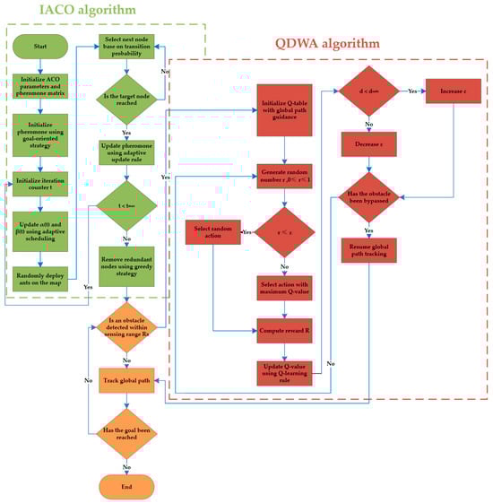
Figure 3. IACO-QDWA algorithm workflow diagram.

During navigation, the robot follows the global path generated by IACO by default. When an obstacle is detected within the sensing range $Rs$, control is immediately transferred to the local planner QDWA to ensure a timely reaction to dynamic environments. Here, $Rs$ denotes the sensing range of the robot, within which obstacles can be detected. After the obstacle leaves the sensing range and local obstacle avoidance is completed, control returns to global path tracking.

The detailed operational steps corresponding to this workflow are summarized in Algorithms 1–3. Algorithm 1 describes the overall IACO–QDWA framework, while Algorithms 2 and 3 present the detailed procedures of the global IACO planner and the local QDWA controller, respectively.

Algorithm 1. IACO–QDWA Hybrid Path Planning Framework

1: Input: start point a, goal point b, sensing range $Rs$, parameters

2: Output: executed collision-free trajectory P

3: Pg ← IACO Global Planning(a,b) (Algorithm 2)

4: Initialize robot motion state $x,y,\theta ,v,\omega$

5: Set local goal ← next waypoint on Pg

6: while not reached goal do

7:  Detect obstacles within $Rs$

8:  if obstacle detected within $Rs$ then

9:   while obstacle detected within $Rs$ do

10:    Run QDWA local planner for one control cycle ()

11:     else

12:     Set local goal ← next waypoint on Pg

13:  else

14:     Track the global path Pg

15:     Update local goal ← next waypoint on Pg

16:  end

17: end

18: return P

Algorithm 2. IACO for Global Path Planning

1: Input: start point a, goal point b, number of ants m, maximum iterations tmax

2: Output: global path Pg

3: Initialize pheromone ${\tau }_{ij}(0)$ (Equation (5))

4: for t = 1 to tmax do

5:  Update $\alpha (t)$, $\beta (t)$ (Equations (7)–(8))

6:  for each ant k = 1 to m do

7:   Compute $P_{ij}^k$ (Equation (1))

8:   Compute ${\eta }_{ij}^{\beta }(t)$ (Equation (2))

9:   Select next node by roulette wheel using $P_{ij}^k$ (Equation (1))

10:  end

11:  Compute $∆{\tau }_{ij}$ (Equation (4))

12:  Update pheromone ${\tau }_{ij}(t+1)$ (Equation (3))

13:  Apply adaptive pheromone update strategy (Equation (6))

14: end

15: Greedy pruning of the best path

16: return Pg

Algorithm 3. QDWA for Local Obstacle Avoidance

1: Input: current motion state $(x,y,\theta ,v,\omega )$, local goal (next waypoint), sensing range $Rs$

2: Output: selected action $A=\{(∆v,∆\omega )\}$ and executed local motion

3: Predict robot motion (Equations (9)–(11))

4: Compute $V_S$, $V_{\mathrm{d}}$, $V_a$ (Equations (12)–(14))

5: Compute dynamic window $V_r$ (Equation (15))

6: Sample $(v,\omega )\in V_r$ and generate candidate trajectories

7: Evaluate trajectories using $J(v,\omega )$ (Equation (16))

8: Construct state vector $S=(d_g,{\theta }_e,d_o,v,\omega )$

9: Select action $A=\{(∆v,∆\omega )\}$ using ε-greed

10: Update velocities: $v$ ← $v+∆v$; $\omega$ ← $\omega +∆\omega$

11: Execute update $(v,\omega )$ and obtain new state $S\prime$

12: Compute reward $R$ (Equations (17)–(22))

13: Update $Q\prime (S,A)$ (Equation (23))

14: return A

5. Experimental Simulation

5.1. Static Path Planning Experiment

The experimental environment was established on a Windows 11 operating system using the MATLAB 2022a simulation platform. Simulations were run on a system with an Intel i7-11700KF, 16 GB RAM, and an NVIDIA GeForce RTX 3060. Numerical simulations were conducted to validate and compare the performance of the IACO. To comprehensively evaluate the algorithmic effectiveness, comparative experiments involving the traditional ACO, the improved ACO reported in [26] (denoted as ACO—[26]), and the proposed IACO were performed on a 20 × 30 two-dimensional grid map. The 20 × 30 grid was selected for these experiments to simulate a more complex environment with a higher number of static obstacles, allowing us to test the algorithm’s performance in denser obstacle configurations. Table 2 summarizes the parameter settings used for the IACO and for ACO—[26].

Table 2. IACO and ACO—[26] parameter settings.

Parameter	IACO	ACO—[26]
Number of ants	50	40
Maximum iterations	100	100
Pheromone influence factor α	1.7	1.5
Heuristic information factor β	3.7	10
Pheromone reinforcement coefficient Q	0.4	1
Pheromone evaporation rate ρ	0.4	0.9
Euclidean distance dab	29.53	29.53
Corner heuristic parameter n	N/A	5
Pheromone allocation weight factor φ	2	3

As shown in Figure 4 and Figure 5, although the traditional ACO is capable of generating a complete static obstacle avoidance path in a simple map, its inherent limitations often cause the algorithm to fall into local optima. Moreover, the resulting path contains numerous turning points, which compromise path smoothness. This issue becomes even more pronounced in complex map environments. In contrast, the ACO—[26] effectively reduces the number of turning points and enhances path smoothness on both simple and complex maps; however, the generated path is still not optimal. The IACO demonstrates clear advantages in both simple and complex obstacle maps by further reducing turning points and improving path smoothness, thereby delivering superior obstacle avoidance performance and significantly enhanced algorithmic efficiency.

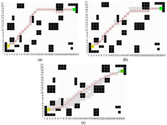
Figure 4. Planned paths of three algorithms in a simple static obstacle map: (a) traditional ACO; (b) ACO—[26]; (c) IACO. Black cells represent static obstacles; the yellow cell indicates the start position; the green cell marks the goal position; gray cells show explored regions; and the red dashed line denotes the planned path.

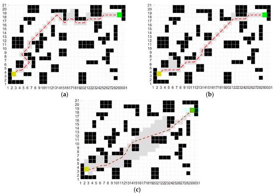
Figure 5. Planned paths of three algorithms in a complex static obstacle map: (a) traditional ACO; (b) ACO—[26]; (c) IACO. Black cells represent static obstacles; the yellow cell indicates the start position; the green cell marks the goal position; gray cells show explored regions; and the red dashed line denotes the planned path.

To further verify the performance of the proposed algorithm, 50 independent runs were conducted for each algorithm in two static experimental scenarios. In each run, the algorithm was initialized with a different random seed while all other conditions remained identical, in order to account for the stochastic nature of ACO. The simulation results of the different algorithms are presented in Table 3 and Table 4.

Table 3. Performance of three algorithms in a simple static obstacle map.

	Average Optimal Path Length	Average Time (s)	Turning Point	Maximum Number of Iterations
Traditional ACO	36.382	3.642	9	35
ACO—[26]	33.799	2.246	8	18
IACO in this study	31.537	1.754	3	7

Table 4. Performance of three algorithms in a complex static obstacle map.

	Average Optimal Path Length	Average Time (s)	Turning Point	Maximum Number of Iterations
Traditional ACO	40.281	7.256	12	43
ACO—[26]	34.346	4.216	9	21
IACO in this study	31.996	3.892	5	9

The simulation results in Table 3 and Table 4 show that the traditional ACO algorithm generates trajectories with a large number of turning points in both the simple and complex static-obstacle environments, reflecting poor path smoothness. This deficiency becomes more pronounced as scenario complexity increases. Although ACO—[26] moderately reduces the number of turning points, its improvement remains limited in cluttered settings. By contrast, the IACO yields only 3 and 5 turning points in the two scenarios, indicating consistently improved geometric smoothness across repeated runs.

Beyond path geometry, IACO also demonstrates clear advantages in efficiency. In the simple scenario, the average optimal path length decreases from 36.382 (traditional ACO) to 31.537, an improvement of 13.3%, while in the complex scenario, the reduction reaches 20.6%. The average computation time is similarly reduced—from 3.642 s and 7.256 s to 1.754 s and 3.892 s—corresponding to decreases of 51.8% and 46.4%, respectively. Combined with an almost 80% reduction in maximum iteration count, these results demonstrate that IACO achieves smoother paths, faster convergence, and substantially improved overall planning performance compared with both traditional ACO and ACO—[26].

5.2. Experimental Study on Local Path Planning

To evaluate the performance of the QDWA algorithm, a set of 30 experiments was conducted in MATLAB 2022a and compared against the traditional DWA through simulation. Each experiment was carried out with a different random seed to reduce the stochastic variability introduced by Q-learning. The experimental environment was configured as a 20 × 20 grid map containing 10 obstacles. The 20 × 20 grid was used here to simulate a simpler environment with fewer obstacles, allowing us to focus on evaluating the algorithm’s responsiveness and real-time decision-making capabilities in scenarios with lower computational demands. The robot’s operating radius was set to 0.5 m, and the obstacle radius was also set to 0.5 m. The maximum linear velocity of the robot was 2 m/s, the maximum angular velocity was $\pi /4$ rad/s, and the maximum acceleration was 0.3 $\mathrm{m}/{\mathrm{s}}^2$. Other parameters are listed in Table 5.

Table 5. The parameter settings.

Parameter	Value
Learning Rate $\lambda$	0.1
Discount Factor $\gamma$	0.95
Exploration Rate $\epsilon$	0.2
Safety Distance dsafe (m)	2
Sensitivity Coefficient $\sigma$	0.6
Step Size dt (s)	0.1
Velocity Resolution (m/s)	0.2
Prediction Time (s)	3
Target Reward Coefficient $k_1$	0.3
Stability Coefficient $k_2$	0.15
Smoothness Coefficient $k_3$	0.15
Turning Coefficient $k_4$	0.1
Obstacle Collision Coefficient	0.3

The comparative results in Figure 6 and Figure 7 and Table 6 indicate that QDWA delivers consistently superior performance over the traditional DWA. As shown in Figure 6, QDWA produces a smoother and more direct obstacle avoidance trajectory, whereas traditional DWA exhibits larger deviations and a longer path.

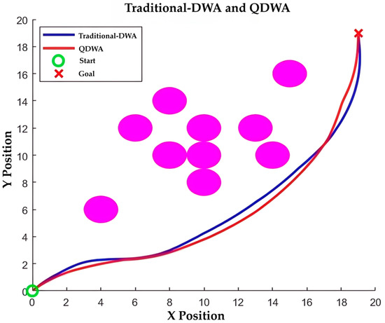
Figure 6. Obstacle avoidance diagram of traditional DWA and QDWA: purple circles indicate obstacles.

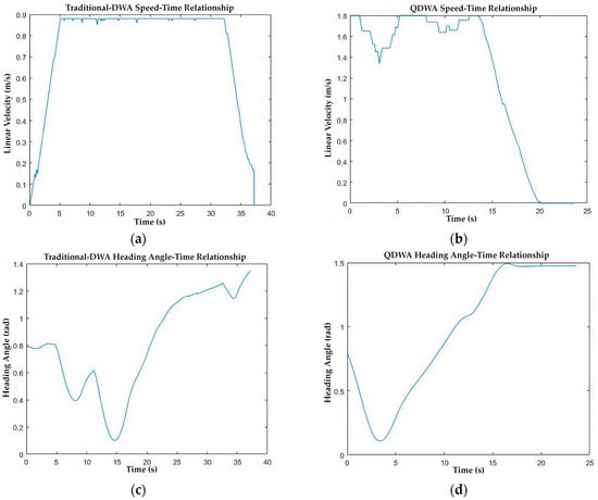
Figure 7. Relationship between speed, heading angle, and time: (a) linear velocity variation in the traditional DWA; (b) linear velocity variation in the QDWA; (c) variation in heading angle in the traditional DWA; (d) variation in heading angle in the QDWA.

Table 6. Two algorithms with 30 sets of experimental runtime.

	Average Running Time (s)	Average Time to Goal (s)
Traditional-DWA	11.212	37.235
QDWA	4.622	20.413

Note: Runtime is wall-clock computation time and includes online Q-learning updates; multi-episode training-to-stability is not included.

The velocity and heading-angle profiles (Figure 7a,d) show that QDWA maintains higher and more stable linear velocities with fewer oscillatory heading adjustments, reflecting more decisive and efficient motion control.

Quantitatively, QDWA reduces the average running time from 11.212 s to 4.622 s (58.8% improvement) and decreases the average time to reach the target from 37.235 s to 20.413 s (45.2% improvement). These results confirm that QDWA achieves better average navigation efficiency and trajectory smoothness across repeated trials, achieving faster and more stable obstacle avoidance compared with the traditional DWA.

5.3. IACO-QDWA Experiment

The IACO algorithm and the enhanced DWA algorithm are integrated to form the hybrid IACO–QDWA framework, while maintaining the original parameter settings of both modules. Here, the 20 × 30 grid size was chosen again to simulate a complex environment with both static and dynamic obstacles. The larger grid size allows for more detailed evaluation of the algorithm’s ability to navigate through a larger and more intricate environment. As illustrated in Figure 8, the proposed IACO–QDWA algorithm successfully performs obstacle avoidance in environments containing both static and dynamic obstacles.

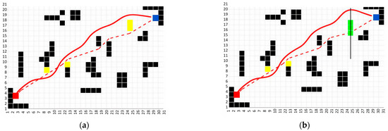
Figure 8. Planned path of IACO-QDWA in a map with low density of unknown obstacles: (a) map with unknown static obstacles; (b) map with unknown dynamic obstacles. Red blocks represent the start position; blue blocks represent the goal position. Black blocks represent static obstacles; yellow blocks represent unknown static obstacles; green blocks represent unknown dynamic obstacles that move vertically along the solid trajectory at a constant velocity $V$. The red dashed line represents the global planned path, and the red solid line indicates the actual executed trajectory.

To further evaluate the obstacle avoidance performance of the IACO-QDWA algorithm in complex dynamic environments, comparative experiments were conducted with a baseline ACO-DWA method obtained by directly combining traditional ACO and DWA, as well as the PSO-DWA algorithm proposed in [27]. In environments with denser obstacles, a total of 30 sets of experiments were performed for two different dynamic obstacle configurations (State 1 and State 2). In State 1, the movement range of the obstacles was smaller, while in State 2, the movement range of the obstacles was larger, making the environment more challenging. All experiments were repeated under identical conditions but with different random seeds to mitigate stochastic effects arising from both ACO and Q-learning. The experiment was considered successful if the robot reached the target point without collision within 45 s; otherwise, it was considered a failure. All algorithm parameters were selected based on common settings in the respective literature and adjusted through the same empirical tuning process to ensure the fairness of the comparison. The experimental results are shown in Figure 9 and Table 7.

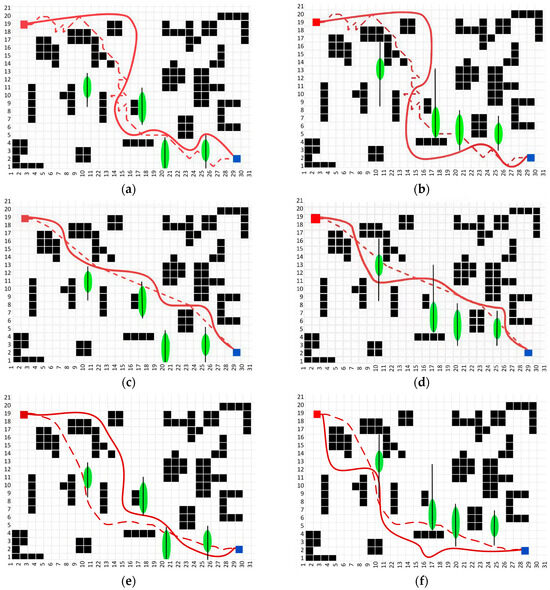
Figure 9. Comparison of optimal path performance of three algorithms on dense obstacle maps: (a) ACO-DWA State 1; (b) ACO-DWA State 2; (c) IACO-QDWA State 1; (d) IACO-QDWA State 2; (e) PSO-DWA State 1; (f) PSO-DWA State 2. Red blocks represent the start position; blue blocks represent the goal position. Black blocks represent static obstacles; green ellipses represent unknown dynamic obstacles that move vertically along the solid trajectory at a constant velocity $V$. The red dashed line represents the global planned path, and the red solid line indicates the actual executed trajectory.

Table 7. Comparison of the three algorithms on data from maps with dense obstacles.

Algorithm	Map	Optimal Path Length (m)	Average Path Length (m)	Average Time to Goal (s)	Average Runtime (s)	Failures	Success Rate (%)
ACO-DWA	State 1	46.627	48.597 ± 3.35	36.247 ± 4.57	5.926	3	90
	State 2	50.061	53.894 ± 4.73	40.016 ± 5.20	8.341	5	83.3
IACO-QDWA	State 1	38.734	40.235 ± 1.85	25.235 ± 1.41	3.881	1	96.7
	State 2	39.983	42.588 ± 2.59	26.133 ± 2.09	4.254	2	93.3
PSO-DWA	State 1	42.544	43.921 ± 2.23	30.432 ± 1.49	2.567	2	93.3
	State 2	44.140	46.044 ± 2.81	31.573 ± 2.16	2.916	2	93.3

Note: Values are reported as mean ± standard deviation over 30 independent runs with different random seeds. The runtime follows the same definition as in Table 6 and refers to the wall-clock computation time.

From the simulation results, it can be observed that in complex dynamic environments, the traditional ACO-DWA algorithm tends to produce detours and fails more frequently during interactions with dynamic obstacles. PSO-DWA can shorten path lengths in some scenarios, but still faces instability in obstacle avoidance under high dynamic conditions. In contrast, IACO-QDWA demonstrates superior overall performance in both states, effectively avoiding dynamic obstacles while maintaining path continuity and stability.

Quantitative results show that, in both State 1 and State 2, IACO-QDWA reduces the optimal path length by approximately 16.9–20.0% and 8.9–9.4%, respectively, compared to traditional ACO-DWA and PSO-DWA. The target reach time is also significantly shortened. Moreover, it has the fewest failure trials, indicating that the method has higher success rates and robustness in complex dynamic environments. Although the computation time of IACO-QDWA is slightly higher than that of PSO-DWA, considering the overall path quality, obstacle avoidance success rate, and stability in high-dynamic scenarios, this additional computational overhead is acceptable.

Overall, the experimental results indicate that IACO-QDWA achieves a more reasonable balance between path quality, obstacle avoidance success rate, and real-time performance on average across multiple independent runs in complex dynamic environments. Compared to traditional ACO-DWA and PSO-DWA, the proposed method exhibits more stable obstacle avoidance behavior and more reliable navigation performance on average across repeated experiments under both dynamic obstacle configurations. It should be noted, however, that in scenarios with relatively sparse dynamic obstacles or limited interactions, the performance advantage of IACO-QDWA may become marginal, while faster methods such as PSO-DWA can provide comparable navigation performance with lower computational cost.

5.4. Ablation Study

To analyze the contribution of each proposed component, an ablation study was conducted in a representative dense dynamic obstacle environment (State 1). In this study, only one component was modified at a time while all other experimental settings were kept identical. Each variant was evaluated using the same experimental protocol and number of trials as in Section 5.3.

Four variants were evaluated: ACO-DWA as the baseline, IACO-DWA with the improved global planner, ACO-QDWA with the Q-learning-enhanced local planner, and the full IACO-QDWA framework. The results are summarized in Table 8.

Table 8. Ablation study results in a dense dynamic obstacle environment (State 1).

Algorithm	Average Path Length (m)	Average Time to Goal (s)	Success Rate (%)
ACO-DWA	48.597	36.247	90
IACO-DWA	42.834	33.983	90
ACO-QDWA	47.916	27.417	93.3
IACO-QDWA	40.235	25.235	96.7

Note: All variants were evaluated under identical experimental settings in State 1. Results for ACO-DWA and IACO-QDWA are reused from Section 5.3.

Comparing ACO-DWA and IACO-DWA shows that the IACO mainly contributes to reducing the average path length (48.597 m to 42.834 m), while its impact on the time to reach the goal and success rate is limited. In contrast, comparing ACO-DWA and ACO-QDWA indicates that Q-learning significantly improves local obstacle avoidance efficiency, leading to a reduced navigation time (36.247 s to 27.417 s) and a higher success rate (90.0–93.3%), with little change in path length.

The full IACO-QDWA framework achieves the best overall performance, with the shortest average path length (40.235 m), the lowest time to reach the goal (25.235 s), and the highest success rate (96.7%). These results indicate that the improved global planner and the learning-based local planner provide complementary benefits, and the observed performance gains arise from their combined integration rather than from a single component alone.

6. Conclusions

In this study, we propose the IACO–QDWA framework, a hybrid path planning approach that integrates the improved ant colony optimization algorithm for global path planning with a Q-learning-enhanced dynamic window approach for local obstacle avoidance. The proposed framework effectively addresses key challenges of traditional methods, particularly in dynamic environments, by combining global path quality with real-time reactive decision-making.

The IACO–QDWA framework enables robots to generate shorter, smoother, and more stable paths in static environments, while maintaining reliable and efficient obstacle avoidance in dynamic scenarios. The global planner provides consistent guidance, and the local planner adapts online to environmental changes, allowing the robot to adjust its trajectory in real-time without sacrificing navigation efficiency.

The experimental evaluation primarily focuses on dynamic obstacles with regular motion patterns to validate the core integration between global planning and local reactive avoidance. In this context, the QDWA module operates purely reactively, without relying on explicit trajectory prediction, thereby enhancing adaptability to various motion patterns. However, the current framework assumes accurate state perception and moderate obstacle dynamics, and its performance may degrade under conditions such as significant sensor noise, high-speed obstacles, or substantial map uncertainty. Future work will address more complex scenarios, including perception uncertainty, human–robot interaction, and highly nonlinear or stochastic obstacle behaviors.

References

- Agarwal, D.; Bharti, P.S. Implementing Modified Swarm Intelligence Algorithm Based on Slime Moulds for Path Planning and Obstacle Avoidance Problem in Mobile Robots. Appl. Soft Comput. 2021, 107, 107372. [Google Scholar] [CrossRef]
- Qin, H.; Shao, S.; Wang, T.; Yu, X.; Jiang, Y.; Cao, Z. Review of Autonomous Path Planning Algorithms for Mobile Robots. Drones 2023, 7, 211. [Google Scholar] [CrossRef]
- Lee, J.; Kim, D.-W. An Effective Initialization Method for Genetic Algorithm-Based Robot Path Planning Using a Directed Acyclic Graph. Inf. Sci. 2016, 332, 1–18. [Google Scholar] [CrossRef]
- Zhang, W.; Wang, N.; Wu, W. A Hybrid Path Planning Algorithm Considering AUV Dynamic Constraints Based on Improved A* Algorithm and APF Algorithm. Ocean Eng. 2023, 285, 115333. [Google Scholar] [CrossRef]
- Liu, C.; Xie, S.; Sui, X.; Huang, Y.; Ma, X.; Guo, N.; Yang, F. PRM-D* Method for Mobile Robot Path Planning. Sensors 2023, 23, 3512. [Google Scholar] [CrossRef]
- Sun, H.; Zhu, K.; Zhang, W.; Ke, Z.; Hu, H.; Wu, K.; Zhang, T. Emergency Path Planning Based on Improved Ant Colony Algorithm. J. Build. Eng. 2025, 100, 111725. [Google Scholar] [CrossRef]
- Zhang, Z.; Yang, H.; Bai, X.; Zhang, S.; Xu, C. The Path Planning of Mobile Robots Based on an Improved Genetic Algorithm. Appl. Sci. 2025, 15, 3700. [Google Scholar] [CrossRef]
- Liu, B.; Jin, S.; Li, Y.; Wang, Z.; Zhao, D.; Ge, W. An Asynchronous Genetic Algorithm for Multi-Agent Path Planning Inspired by Biomimicry. J. Bionic Eng. 2025, 22, 851–865. [Google Scholar] [CrossRef]
- Ahmad, J.; Wahab, M.N.A.; Ramli, A.; Misro, M.Y.; Ezza, W.Z.; Hasan, W.Z.W. Enhancing Performance of Global Path Planning for Mobile Robot through Alpha–Beta Guided Particle Swarm Optimization (ABGPSO) Algorithm. Measurement 2026, 257, 118633. [Google Scholar] [CrossRef]
- Yuan, L.; Luo, J. Approach to Global Path Planning and Optimization for Mobile Robots Based on Multi-Local Gravitational Potential Fields Bias-P-RRT*. J. Comput. Sci. 2025, 92, 102718. [Google Scholar] [CrossRef]
- Zhang, J.; Qiao, J.; Huang, K.; Zhang, M. An Optimized Hierarchical Path Planning Method Based on Deep Reinforcement Learning for Mobile Robots. Expert Syst. Appl. 2026, 298, 129736. [Google Scholar] [CrossRef]
- Wang, Y.; Fu, C.; Huang, R.; Tong, K.; He, Y.; Xu, L. Path Planning for Mobile Robots in Greenhouse Orchards Based on Improved A* and Fuzzy DWA Algorithms. Comput. Electron. Agric. 2024, 227, 109598. [Google Scholar] [CrossRef]
- Lin, H.-I.; Shodiq, M.A.F.; Hsieh, M.F. Robot Path Planning Based on Three-Dimensional Artificial Potential Field. Eng. Appl. Artif. Intell. 2025, 144, 110127. [Google Scholar] [CrossRef]
- AbuJabal, N.; Baziyad, M.; Fareh, R.; Brahmi, B.; Rabie, T.; Bettayeb, M. A Comprehensive Study of Recent Path-Planning Techniques in Dynamic Environments for Autonomous Robots. Sensors 2024, 24, 8089. [Google Scholar] [CrossRef]
- Ravankar, A.; Ravankar, A.A.; Kobayashi, Y.; Hoshino, Y.; Peng, C.-C. Path Smoothing Techniques in Robot Navigation: State-of-the-Art, Current and Future Challenges. Sensors 2018, 18, 3170. [Google Scholar] [CrossRef]
- Türkkol, B.Z.; Altuntaş, N.; Çekirdek Yavuz, S. A Smooth Global Path Planning Method for Unmanned Surface Vehicles Using a Novel Combination of Rapidly Exploring Random Tree and Bézier Curves. Sensors 2024, 24, 8145. [Google Scholar] [CrossRef] [PubMed]
- Li, D.; Wang, L. Research on Mobile Robot Path Planning Based on Improved Q-Evaluation Ant Colony Optimization Algorithm. Eng. Appl. Artif. Intell. 2025, 160, 111890. [Google Scholar] [CrossRef]
- Ye, F.; Duan, P.; Meng, L.; Xue, L. A Hybrid Artificial Bee Colony Algorithm with Genetic Augmented Exploration Mechanism toward Safe and Smooth Path Planning for Mobile Robot. Biomim. Intell. Robot. 2025, 5, 100206. [Google Scholar] [CrossRef]
- Tao, B.; Kim, J.-H. Mobile Robot Path Planning Based on Bi-Population Particle Swarm Optimization with Random Perturbation Strategy. J. King Saud Univ. Comput. Inf. Sci. 2024, 36, 101974. [Google Scholar] [CrossRef]
- Ye, L.; Wu, F.; Zou, X.; Li, J. Path Planning for Mobile Robots in Unstructured Orchard Environments: An Improved Kinematically Constrained Bi-Directional RRT Approach. Comput. Electron. Agric. 2023, 215, 108453. [Google Scholar] [CrossRef]
- Xin, J.; Guo, P.; Li, H.; D’Ariano, A.; Liu, Y. Dual-Mode Guided Reinforcement Learning for Decentralized Lifelong Path Planning of Multiple Automated Guided Vehicles in Robotic Mobile Fulfillment Systems. Comput. Ind. 2026, 174, 104416. [Google Scholar] [CrossRef]
- Liu, L.; Wang, X.; Yang, X.; Liu, H.; Li, J.; Wang, P. Path Planning Techniques for Mobile Robots: Review and Prospect. Expert Syst. Appl. 2023, 227, 120254. [Google Scholar] [CrossRef]
- Sánchez-Ibáñez, J.R.; Pérez-del-Pulgar, C.J.; García-Cerezo, A. Path Planning for Autonomous Mobile Robots: A Review. Sensors 2021, 21, 7898. [Google Scholar] [CrossRef] [PubMed]
- Wang, Y.; Tong, K.; Fu, C.; Wang, Y.; Li, Q.; Wang, X.; He, Y.; Xu, L. Hybrid Path Planning Algorithm for Robots Based on Modified Golden Jackal Optimization Method and Dynamic Window Method. Expert Syst. Appl. 2025, 282, 127808. [Google Scholar] [CrossRef]
- Tong, S.; Liu, Q.; Ma, Q.; Qin, J. Integrating Deep Reinforcement Learning and Improved Artificial Potential Field Method for Safe Path Planning for Mobile Robots. Robot. Intell. Autom. 2024, 44, 871–886. [Google Scholar] [CrossRef]
- Zhang, T.; Wu, B.; Zhou, F. Research on Improved Ant Colony Algorithm for Robot Global Path Planning. Comput. Eng. Appl. 2022, 12, 2120–2127. [Google Scholar]
- Yang, Z.; Li, N.; Zhang, Y.; Li, J. Mobile Robot Path Planning Based on Improved Particle Swarm Optimization and Improved Dynamic Window Approach. J. Robot. 2023, 2023, 6619841. [Google Scholar] [CrossRef]
Disclaimer/Publisher’s Note: The statements, opinions and data contained in all publications are solely those of the individual author(s) and contributor(s) and not of MDPI and/or the editor(s). MDPI and/or the editor(s) disclaim responsibility for any injury to people or property resulting from any ideas, methods, instructions or products referred to in the content. |
© 2026 by the authors. Licensee MDPI, Basel, Switzerland. This article is an open access article distributed under the terms and conditions of the Creative Commons Attribution (CC BY) license.