Abstract
This work addresses the issue of estimating air pollution maps for urban areas. Spatially dense maps of air pollution can be calculated using physical models, such as ADMS-Urban; however, due to the high computational cost of such models, maps are verified with low temporal resolution (such as monthly or yearly averages). We investigate the feasibility of using machine learning models to predict air pollution maps based on historical data and current measurements from a limited number of monitoring stations. The models are trained on spatially dense pollution maps generated by physical models, along with corresponding measurements from monitoring stations and selected meteorological data. We evaluate the performance of the models using real-world data from a central district in Wrocław, Poland, considering various pollutants such as , , CO, VOC, and NOx, presented on spatially dense pollution maps with ca. points with a 10 × 10 m grid. The results demonstrate that the proposed method can effectively predict air pollution maps with high spatial resolution and a fast inference time, making it suitable for generating pollution maps with significantly higher temporal resolution (e.g., hourly) compared to physical models. We also experimentally demonstrated that PM10, CO, and VOC pollution models can be built based on measurements from monitoring stations only with similar, and in the case of CO, higher, accuracy than using measurements from , CO, and VOC monitoring stations, respectively.
1. Introduction
Nitrogen oxides (NOx), carbon monoxide (CO), fine particulate matter (), and volatile organic compounds (VOC) are common air pollutants, and NOx and VOC react under sunlight to form ozone. These pollutants, particularly and ozone, negatively impact human health [1,2,3,4]. Sources of air pollution in urban areas are vehicle traffic and heating of houses in populated zones [3,5]. The sources of and are fuel combustion, traffic, and mineral dust (reconstructions). Secondary sources of , formed in the atmosphere, are sulfates and nitrates that arise from industrial and vehicle emissions [6]. The primary source of NOx in urban areas is the combustion of fossil fuels, primarily from road transport and industrial and commercial activities, including power plants, factories, and heating systems. Carbon monoxide (CO) in urban areas is the result of the incomplete combustion of fossil fuels (traffic and power plants) and domestic activities such as burning wood or charcoal. Volatile organic compounds (VOCs) are the main precursors of ozone and particulate matter [7].
Forecasting the level of air pollution in cities and publishing information on the scale of air pollution is crucial, as it can have a significant impact on public health, mobilizing actions aimed at improving the comfort and health safety of people’s lives in urban agglomerations. Thus, precise methods are needed to assess exposures to air pollution in environmental epidemiological studies [7,8,9]. The work of [10] provides a bibliographic overview of publications addressing various aspects of atmospheric pollution problems in large urban agglomerations. Ref. [11] provides an overview of k-means and hierarchical clustering techniques to analyze air pollution.
The article [8] reviews various aspects of creating spatial models of atmospheric pollution, depending on the sources of observations that serve as the basis for building the models, with a primary focus on land data (Land Use Regression approach). The authors claim, among others, that models based on fixed-site monitoring data generally perform better than those developed using mobile monitoring stations.
In [12], the authors use meteorological parameters, traffic data, and pollutant information from nearby monitoring stations from the previous four years as input to a pollutant model. The computational experiments concerned with the simulation of the concentrations of , and at two sites in Stuttgart use Machine Learning methods (ridge regression, support vector machines, tree-based random forest, extra tree regressor and extreme gradient boosting). They concluded that pollutant information from a nearby station has a significant effect on predicting pollutant concentrations. The paper [13] demonstrates the superiority of nonlinear shallow regression networks over linear models in the task of interpolation of points in the spatial prediction of air pollution. Data from 4 to 13 existing air quality monitoring stations, depending on the type of air pollutant, were used for spatial modeling of the Athens metropolitan area. In this work, for each pollutant, a specific monitoring station is the target site, and the measurements at the remaining monitoring sites are used to estimate the level of the pollutant concentrations at the target. Data were collected over a period of approximately 12 years. Observations from the last two years of this period were used as test data, and training data contained between 22,000 and 44,000 observations, depending on the type of pollution.
A comprehensive overview of deep machine learning methods can be found in [14,15]. However, deep methods require a large amount of data to achieve good prediction results [4].
In the work [16], meta-models for spatial pollution prediction were developed. This paper presents a method for replacing the complete ADMS-Urban [17] model for the French city of Clermont-Ferrand with a fast-calculated surrogate model for the prediction of NOx and grid maps as functions of day and hour. The output of the ADMS-urban model is first projected onto a reduced subspace using PCA. The relationships between the input data (wind speed, wind direction, temperature, cloud cover, solar radiation, and background pollution concentrations) and the coefficients obtained from the projection are then approximated using Kriging functions or radial basis functions (RBFs).
The work [18] proposes a regression model for the generation of pollution maps, designed to predict the concentration of several pollutants (, , , ) at single points on the map. Regression models are based on data from monitoring stations, forecasts of atmospheric conditions, land cover data, and traffic estimates. The authors employ this approach to predict large-scale (country- or even continent-level) pollution maps and claim that the method can also be applied at the urban scale. However, the paper does not provide any experimental results for the quality of the urban-scale pollution maps prediction.
Our goal in this work is to investigate the feasibility of using machine learning regression models to create approximate pollution maps on the urban scale. We compare two types of models: multi-output regression models, which directly predict pollution values at all map points, and simple regression models, which predict pollution values at single map points. The former type of models is realized as the MLP-PCA model described later in this paper, while the latter type of models is realized as Light Gradient Boosting Machines (LGBM). The output of the multi-output regression model is a complete pollution map, while generating a complete pollution map using the simple regression model requires applying the model to each map point separately, as proposed in [18]. We compare the quality of pollution maps generated by both types of models using real-world data from a central district in Wrocław, Poland.
The purpose of the regression models investigated in this work is to replace the precise but computationally expensive physical model used by Lemitor to generate pollution maps for , CO, VOC, NOx, and . The surrogate models [19,20,21] should be able to generate pollution maps with significantly higher temporal resolution (e.g., hourly) than the physical models, based on measurements from 11 monitoring stations, possibly supplemented with selected meteorological data.
2. Materials and Methods
2.1. Study Area
Our study area is a real urban location—a central district in Wrocław (a large city in Poland). It consists of a part of the city center, as well as large residential and park areas. Several major roads pass through this area. Careful monitoring of air pollution in this area, where many people spend their time during the day or reside permanently, is a crucial element in consciously caring for the health of Wrocław residents.
The map in Figure 1 shows the area of interest monitored by Lemitor. This area is located between longitudes 17.0070° E and 17.1290° E and latitudes 51.0933° N and 51.1346° N and is surrounded by the canals and channels of the Oder River. It consists of two islands divided by the Old Oder River.
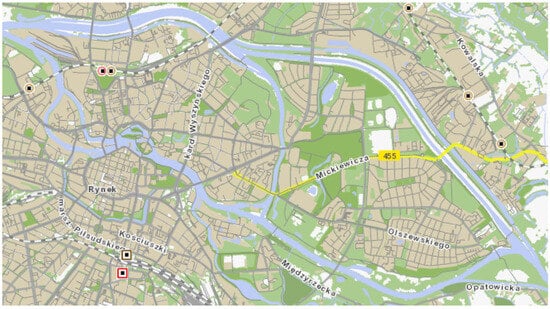
Figure 1.
The map of the area of interest monitored by Lemitor (see https://gis.um.wroc.pl/imap/ (accessed on 10 October 2025)).
The key reasons behind changes in the levels of urban air pollutants in the study area were traffic emissions and fossil fuel heating.
2.2. Data
The monitored pollutants are , , NOx, CO, and VOC. The models we use in our work are based on data that create unevenly sampled time sequences, while each observation contains a spatially uniformly sampled map of monitored air pollutants. Due to the different time intervals between observations, they are treated as independent observations. These maps were obtained by Lemitor, and the methods used to generate them are beyond the scope of this work. The aim of this work is to investigate the feasibility of quickly creating flexible surrogate models that approximate grid maps, based on current data from a small number of stationary measurement stations and, optionally, current weather data. The data on the characteristics of the terrain are constant over time. Data for each pollutant consist of 696 dense m grid point maps of the monitored area obtained by Lemitor. Each map contains information about pollution values at the 194,477 grid points at a given time (one of a set of 696 timestamps).
In addition, detailed characteristics of each point on the terrain map are available, including geographic coordinates, elevation of the terrain, and type of terrain (percentage of roads, buildings, and greenery within a 10 × 10 m grid area). Observed pollution levels are seasonal, depending on the time of year [17].
The timestamp collection (T) spans a period of one year. For the months of January through November inclusive, pollution maps are available for Tuesday, Thursday, Saturday, and Sunday of a selected week, corresponding to the hours 00, 03, 06, 07, 08, 11, 12, 13, 15, 16, 17 and 21. Thus, each month (January to November) is represented by 48 maps. In addition, December includes maps for the entire week, from Monday to Sunday, with 1-h intervals, totaling 168 maps. This yields a total of 696 maps (numbered 0 to 695) for each of the pollutants analyzed, collected over the course of one year. All pollution values in both tables and figures are recorded in the same units, namely μg/m3. Table 1 provides elementary statistics for the , , CO, VOC, and NOx data. It should be noted that the values quoted refer only to available data, which do not fully cover the entire year. Therefore, based on the available data, we can formally calculate all statistics, taking into account local divisions based on space and time. Due to the limited number of representative data points, these results are likely to be unreliable.

Table 1.
Elementary statistics for , , CO, VOC, and NOx pollutants (in μg/m3).
The Pearson correlation coefficients (PCC) between and , CO, VOCs, and NOx are 0.999, 0.777, 0.842, and 0.42, respectively. The correlation coefficients between station measurement and corresponding measurements from , CO, VOCs, and NOx stations are 0.9999, 0.545, 0.633, and 0.339, respectively.
The statistics values for and in Table 1 are very similar to each other. The value of when the values of the terrain maps are replaced by the values is close to 1, or more precisely . For individual months of the year, this value ranged from 0.9993 in December to 1.0 in July. The mean absolute percentage error (MAPE) for such replacement is equal to , RMSE is equal to 0.21 μg/m3, MAE is equal to 0.077 μg/m3, and the maximum error is less than 5.21 μg/m3.
Some experiments on CO led us to investigate the extent to which predictions can be based solely on measurements from stations for CO and other pollutants, such as VOC and NOx.
2.3. Machine Learning Models
The learning process will be based on historical data, i.e., previously calculated pollution maps of the monitored area, determined using a precise physical model, together with input data relating to a specific map (i.e., relevant measurements from monitoring stations and weather data). In this paper, we apply two machine learning models.
- Neural networks in the form of a multilayer perceptron (MLP) [22] combined with the reduction in dimensionality of the complete-model output, which is first projected onto a reduced subspace using the principal component analysis method (PCA) [23,24].
- Tree-based models in the form of Light Gradient Boosting Machines (LGBM) [25].
This choice of surrogate model types was driven by the need to find efficient and fast solutions that could operate almost continuously when applied to regression problems with extremely high output dimensions. We also considered the availability of software compatible with the Python 3.10 language. Another important factor was the relative stability of the methods—meaning low sensitivity to small changes in the model input—as well as the ease of selecting hyperparameters. This decision was preceded by extensive experimental research, which, in addition to the solutions we selected, included MLP networks without output dimension reduction, linear methods with regularization (Ridge regression), nearest neighbor methods (k-NN), and various types of ensemble tree regressors.
2.3.1. MLP with PCA
In this approach, principal component analysis (PCA) is used to reduce the dimensionality of time-dependent vectors that contain geospatial data from an urban area.
The structure of the neural network was experimentally selected to suit the size of the data. The input of the network consists of eleven measurements from the official pollutant monitoring station from the time point of view (, , NOx, CO, or VOC) and two meteorological parameters: humidity and direction of the wind.
The selected number of principal components (PC) determines the size of the MLP network output.
The MLP network with two hidden layers containing 200 neurons each with the ReLU activation function, i.e., , and with linear units in the output layer was selected. The MLP regression network was applied using the Scikit-learn MultiOutputRegressor with MLPRegressor [26], along with its optional parameters, specifically the Adam optimizer (see https://scikit-learn.org/(accesed 10 October 2025)).
The maximum number of iterations has been set as 5000, which ensures good convergence with relatively small errors for training sets of different lengths (196 to 624). Due to the small number of observations (pollution levels on the terrain map) relative to their size, this paper proposes a simple yet variant scheme for dividing the data into training and testing data. The method of selecting the model’s hyperparameters was simplified to a bare minimum. The network dimension, the number of layers, and the number of neurons in each layer were selected based on several experiments that involved randomly dividing the data into training and testing sets, and these parameters remained unchanged thereafter. However, the MLP network hyperparameters were set as optional. The number of the largest PC used for the reduction in dimensionality of the output map was determined based on the first 200 observations and depends on the type of pollution. The number of principal components considered was 20, 30, 40, 40, 50, or 60. The five-fold cross-validation method was applied to the chosen data set with MAE taken as criterion. The number of components obtained by the cross-validation procedure ensured that the cumulative explained variance ratio captured by the given number of principal components was, in our experiments, greater than 0.99. The number of PCs retained for VOC and NOx was set to 50 and 60, respectively, and in the remaining cases, .
Computations were performed on two Intel(R) Xeon(R) Silver 4114 CPUs, each with 2.20 GHz and 40 threads. The training time of a single network depended on the number of principal components and the input size, ranging from a few seconds to several seconds.
Additionally, the linear model was implemented in Scikit-learn using the Ridge procedure, with the same input and output data as the full MLP-PCA model, i.e., without reducing the output dimension. Comparing the results of both models allowed us to control the necessity for the nonlinear MLP-PCA model.
2.3.2. Tree-Based Models (LGBM)
As an alternative approach to MLP-based methods, the authors proposed using one of the classic machine learning models, Tree-Based Light Gradient Boosting Machines, to examine how well all the mentioned pollutants can be predicted using a simpler model than neural networks, as applied to the high-dimensional regression problem we are dealing with here.
LGBM is an acronym for Light Gradient Boosting Machine. A highly efficient gradient-boosting decision tree model is presented in [25]. A major advance of LGBM compared to other Gradient Boosting Trees, such as XGBoost [27], is the way the single tree grows. Typical decision tree learning algorithms grow trees by level (depth-wise), while LGBM grows trees leaf-wise, helping to achieve lower loss, better accuracy, and numerical efficiency.
In the experiments presented, no single LGBM model was trained for the entire map. The authors divided the entire terrain into four clusters: roads, buildings, greenery, and miscellaneous areas. The reason for this is the hope that four smaller and specialized models should provide more accurate results than one considerably larger model.
The input feature vector for the LGBM approach consisted of measurements from all eleven monitoring stations and was enriched with additional features, including hour, day of the year, wind speed, wind direction, temperature and spatial coordinates (longitude and latitude). Compared to the MLP approach, the feature vector is then extended, but the output is a single value.
The hyperparameters of the LGBM model were optimized using the Randomized Search method. The combinations of parameters considered in the search were given as:
- Number of boosted trees: {100, 500, 900, 1100, 1500}
- Maximum tree depth for base learners: {2, 3, 5, 10, 15}
- Boosting learning rate: {0.05, 0.1, 0.15, 0.20}
The best set of parameters found was: Number of trees boosted equal to 500, maximum depth equal to 10, and learning rate equal to .
The model was trained on a 31-core AMD Ryzen 9 3950X 16-Core Processor machine. The approximate training time of all 19 variables in the data split was 15 h. The separate variant training time was less than 50 min.
The fact that we can use measurements from monitoring stations to model the levels of various air pollutants is not a general property, but rather an indication of the specificity of the pollutants present in a given area. For example, in the paper [28] it is shown that in the London area, measurements in random forest models are strongly related to values and, to a lesser extent, to NOx levels. In our case, due to the similarity between and pollution levels, could be chosen instead of , depending on needs and possibilities.
3. Results
Nineteen variants of training data were considered, each consisting of a sequence of observations in succession over time. The first column of Table 2 provides the content of the best selected training sets, indicating the starting and ending observation numbers for each case. For example, data from 0–336 included 336 observations available from the beginning of the year, i.e., starting from grid map labeled by 0 and ending by the grid map labeled by 335. The solution obtained on a given training set is tested on five (in the case of MLP-PCA) or four (in the case of LGBM) increasing data sequences. The longest of these encompasses the remaining time-ordered maps. The remaining four are limited to the first 30, 50, 80, and 100 elements of the large test set. In our 0–336 example, these are sets 336–365 (T1 = 30), 336–385 (T2 = 50), 336–415 (T3 = 80) and 336–435 (T4 = 100). The global test applies to the largest testing set, yielding an average result for all remaining data. In the example considered, this interval is 336–696.
Table 2.
prediction results using MLP-PCA with (in μg/m3).
This repeated testing on an increasingly longer sequence of grid maps is intended to estimate how average errors change as the prediction horizon lengthens. In other words, it will be possible to assess the prediction time frame that will ensure a specific level of prediction error. The error measures considered are mean absolute error (MAE) and root mean squeezed error (RMSE). All error values in tables and figures are shown in the same units, namely μg/m3.
3.1. Spatiotemporal Prediction Results for
The pollution prediction errors based on the values of 11 measurement stations are shown in Table 2. denotes the number of principal components used.
The numerical results in Table 2 demonstrate that the choice of data used to determine the principal components matters, as these components encompass the spatial relationships of the modeled pollutants, which depend on time, in particular on season. The subsequent rows in Table 2 refer to the training data, which include dates ending in the following months: April, May, June, etc. up to the end of November. The global test results show model errors for periods from May, June, and so on, all the way to the end of the year. Significantly better errors are generally observed in the subsequent columns of the Table, which present prediction results for shorter time periods (e.g., T2 covers data from one month, T4 from two months). The errors in such cases are usually much smaller. For example, maps from July are best predicted using data from May and June. However, since data from each month are scarce in our case, the 88–288 range already contains sufficient data, additionally not including January and February, which are typically cold months in Wrocław. Naturally, it was not possible to display all variants in Table 2; however, some examples will be presented later in the paper.
Furthermore, for predictions relating to later periods of the year, smaller training sets, in our case containing only sequences of exactly 200 terrain maps, yield worse results (not shown in Table 2) than those obtained based on observations that include all previous data. In addition to the results presented in Table 2, we also computed . The values ranged from 0.988 (for the training set 0–432) to 0.995 (for the training set 0–528). In the case of global results (the Global test columns in Table 2), the normalized MAE values (NMAE), i.e., the MAE values divided by the average values corresponding to the periods in which MAE was determined, ranged from 5.5% to 9.9%.
Furthermore, it is easy to notice (see columns T1,T2, T3, T4 in Table 2) that for predictions with an horizon not exceeding 100, which in the case of the data considered covering a period of approximately two months, the MAE and RMSE errors are definitely smaller than in the global tests.
It should be emphasized that the best value achieved, 0.995, was related to the accuracy of the model in predicting all 168 maps for the December time stamps, despite the training set including data from earlier months of the year. When predicting the pollution map for individual time stamps, results can vary slightly depending on the variability of the pollution values at each individual time stamp.
Figure 2 shows the pollution map 546, 12 December, Monday, 18:00 (6:00 PM). Comparing this map with the road locations in Figure 3 indicates where high levels of pollution are observed over that time. The pollution reconstructions for only one map at 6:00 PM, 12 December, Monday (no. 546) are based on the (0–196) data set and the (0–528) data set, which gave with , , and with , , respectively. The corresponding reconstruction errors, in the same order, are shown in Figure 4.
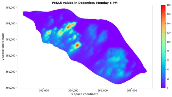
Figure 2.
pollution map for 12 December, Monday, at 6:00 PM. Spatial coordinates are given in the ETRF2000-PL/CS92 coordinate system (EPSG code 2180).
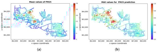
Figure 3.
(a) mean true values and (b) corresponding prediction errors (MAE) for roads (in μg/m3). Spatial coordinates are given in the ETRF2000-PL/CS92 coordinate system (EPSG code 2180).
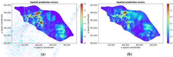
Figure 4.
Spatial prediction errors (in μg/m3) obtained for prediction for map 546, 12 December, Monday, at 6:00 PM (a) based on training set (0–196) and (b) based on training set (0–528).
Figure 5 shows the variation of the approximation errors (MAE) for individual pollution maps determined by the surrogate model for a specific date and time. The values in Table 2 provide the average error values for the terrain map over selected time intervals. It should be noted that the variability presented in Figure 5 is not large compared to the global MAE value.
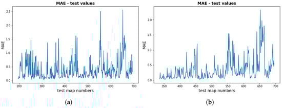
Figure 5.
Individual MAE test values (in μg/m3) for (a) training set (0–196) and for (b) training set (0–336).
The accuracy of the pollution level predictions depends on the type of terrain. Studies have shown that the larger error rate is typically associated with higher levels of pollution and greater variability related to the time of day, as well as possibly the season.
Road traffic areas are usually associated with higher levels of pollution and higher prediction errors. Table 3 shows the results obtained for the observation periods from which the data were used in the testing process.
Table 3.
prediction results using MLP-PCA (PC = 30) for roads only (in μg/m3).
Figure 3 illustrates the general dependence of the mean prediction error (MAE) on the mean level of pollution at the points of the terrain grid corresponding to the roads for training data (0–336), that is, data from the period January to July and tested on other maps (from August to December). In this case was obtained with MAE = 0.46 μg/m3 and . Small errors are also characteristic of predictions in the summer months, specifically, June, July, and August, where the modeled average values are lower than in the other months. The RMSE errors for pollution prediction based on the combined LGBM approach are shown in Table A1.
3.2. Spatiotemporal Prediction Results for
Table A2 and Table A3 present the results of the prediction experiments for carried out according to the same scheme as for , based on values obtained from the measurement stations and , respectively. Based on measurements from the monitoring stations, the best values ranged between 0.987 (for the training set 88–288) and 0.998 (for the training set 0–528). The results using measurements are typically only slightly worse than those based on . The values ranged between 0.985 (for the 88–288) and 0.997 (for the 0–528 training set). It should be noted that the best value achieved of was related to the accuracy of the model in predicting the maps for the December time stamps, although the training set included only data from earlier months of the year.
Due to the large similarity in the observed particulate matter levels, the prediction results for differ from those for in terms of small random noise. Thus, prediction errors can be based on both the and the monitoring stations. However, the normalized MAE ranged between 4.2–9.5%, and 3.8–9.4%, for measurements and , respectively. The pollution prediction errors for based on the combined LGBM approach are similar to those of the prediction values of .
3.3. Spatiotemporal Prediction Results for CO
The advantages of selecting training data according to the season also refer to predicting CO levels in the terrain grid. Table A4 presents CO prediction values based on information from actual measurements at the station. The errors in CO prediction are an order of magnitude larger than those in air dust prediction, but the measured or estimated CO values are also an order of magnitude larger. The errors normalized to the mean values are of similar order in both cases.
The corresponding results based on the actual CO measurements are presented in Table A5. Quite often, they are larger than in the case where the input to the model consists of measurements.
In summary, the best values obtained for measurements ranged between 0.817 for the 88–288 training set and 0.902 for the 0–528 training set. Normalized MAE values are in the range between 19% and 26.7%. The results using CO measurements are definitely worse. The values of are in the range of 0.708 and 0.858, and the normalized MAE ranged between 28.1% and 43.8%. Similarly to the case of the predictions and , the best results were achieved for the December maps, probably because during this period the higher prediction errors are compensated for by a much wider range of variability in the modeled CO values.
Figure 6 shows the relationship between the true values (the values of the physical model) and the prediction results for a single map (546, 12 December, Monday, 6:00 PM), with training on the 0–196 training data.
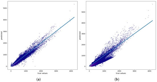
Figure 6.
(a) CO true values versus MLP-PCA model-predicted values using measurements from monitoring stations, and (b) CO true values versus MLP-PCA model-predicted values using CO measurements from monitoring stations for one map prediction. All values are given in μg/m3.
Figure 7 shows the prediction results for map 546 (12 December, Monday, at 6:00 PM) and the corresponding true values.
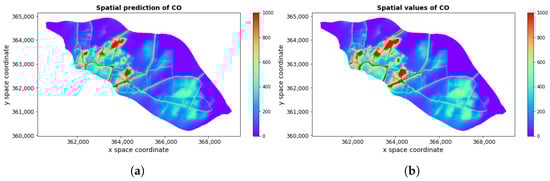
Figure 7.
(a) Spatial predictions obtained for CO based on training set (0–196) and (b) corresponding true values (in μg/m3). Spatial coordinates are given in the ETRF2000-PL/CS92 coordinate system (EPSG code 2180).
The advantage of using measurements over CO measurements is a very interesting phenomenon that cannot be explained without a more detailed analysis of the chemical processes that occur in the environment and the CO measurement methods at the measurement stations. When using CO measurements from monitoring stations for spatial CO data reconstruction, the results obtained were similar in precision to those of the linear model with regularization . The values of the monitoring stations certainly gave better results than linear regression.
In Table A6, the prediction errors for the CO pollutant have been collected based on the combined LGBM approach. The error levels obtained are high, typically at least about twice as large as in the MLP-PCA model.
3.4. Spatiotemporal Prediction Results for VOC
The advantages of selecting training data according to the season also refer to predicting the VOC levels of the terrain grid using measurements from the measurement stations. Table A7 provides VOC prediction values using information from actual measurements of the station. The corresponding results based on the actual VOC measurements are given in Table A8. The prediction errors are greater than those obtained with the prediction based on .
The best values obtained for the measurements ranged between 0.877 for the 88–288 training set and 0.955 for the 0–528 training set. The normalized MAE are in the range 13.3% and 23.2%. The results using VOC measurements are less accurate. The values of are in the range of 0.864 and 0.927, and the normalized MAE ranged between 19.6% and 31.4%. As in the case of , , and CO, the best results were achieved for the December maps.
Figure 8 shows the VOC prediction results for one separate map (12 December, Monday, 6 PM). For the measurements we get , μg/m3, and the average VOC is equal to 24.96 μg/m3 (normalized ). The corresponding values for measurements from the VOC station were , μg/m3 and normalized . The prediction errors for VOC based on the combined LGBM approach are presented in Table A9. The errors appear to be approximately at least twice as severe as those of the MLP-PCA approaches.
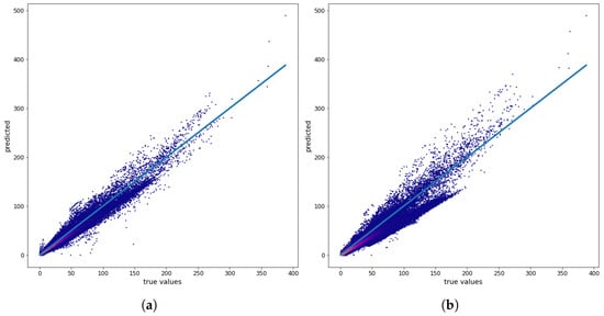
Figure 8.
(a) VOC true values versus MLP-PCA model-predicted values using measurements from monitoring stations and (b) VOC true values versus MLP-PCA model-predicted values using VOC measurements from monitoring stations for 546 map (12 December, Monday, at 6:00 PM) prediction. All values are given in μg/m3.
3.5. Spatiotemporal Prediction Results for NOx
Table A10 and Table A11 provide NOx prediction values using information from actual measurements of the and NOx measurement stations, respectively. NOx has similar statistics to VOC (see Table 1), but it has a wider range of variability. However, even though the MAE prediction errors obtained from the measurements are slightly larger than those obtained from the NOx monitoring station measurements, the RMSE errors differ significantly, showing that, in this case, the use of the measurements from the monitoring stations can generate large spatial errors.
The best values obtained for NOx based on the measurements ranged between 0.859 for the training set 0–196 and 0.874 for the training set 0–528. Normalized MAE values range from 29.7% to 37.7%. The results using NOx measurements are more accurate. The values of are in the range of 0.897 (for the training set 0–288) and 0.928 (for the training set 0–528). Normalized MAE ranged from 22.9% to 34.8%.
Figure 9 shows the relationship between the true values (the values of the physical model) and the prediction results for a single map (no. 546, 12 December, Monday, at 6:00 PM) using the training set 0–196. In the case of other pollutants, the spread of errors was significantly smaller than in the case of NOx.
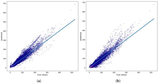
Figure 9.
(a) NOx true values versus MLP-PCA model-predicted values using measurements from monitoring stations, , and (b) NOx true values versus MLP-PCA model-predicted values using NOx measurements from monitoring stations, for map 546 (12 December, Monday, 6:00 PM) prediction. All values are given in μg/m3.
In the case of NOx prediction, the LGBM approach seems to perform much worse than the MLP-PCA-based approaches.
4. Discussion and Conclusions
This article addresses the important and practically relevant problem of forecasting air pollution in cities with very high spatial and temporal resolution. The proposed approach uses several hundred (200 to 500) previously prepared runs of the original physical model (such as ADMS-URBAN [16,17]) treated as historical data. Based on these runs and using measurements from monitoring stations and weather information, a surrogate model is trained using machine learning methods.
This solution allows for replacing the complex original model in a time period where historical data can be considered current, and the physical model is only run when the urban system changes.
This approach significantly reduces computational costs compared to physical models such as ADMS-Urban and enables the generation of near-real-time pollution maps, which is important for environmental warning systems and air quality management.
The input data for the training of the surrogate model are measurements from stations monitoring the levels of atmospheric pollutants (, , CO, VOC, NOx) associated with historical pollution maps. Due to the high precision required for spatial modeling, since the terrain map included 194,477 points, it was decided to reduce the output dimension using PCA in the model based on a deep neural network (MLP-PCA). In the paper, we compare the MLP-PCA multi-output approach with the Light Gradient Boosting Machine (LGBM) one-output methodology. The models produce pollution maps at a high spatial resolution of 10 m × 10 m grid points, but only MLP-PCA is a multi-output model.
A multi-output model could be fully replaced by approximately 200,000 copies of single-output models. However, even scanning a space consisting of many grid points is much more time-consuming than the multi-output approach.
It is worth noting that combining a regression model with output dimensionality reduction is not a common practice. In fact, models based on neural networks (and other models used in machine learning) are often combined with PCA dimension reduction; however, this reduction applies to the input data, not the output from the network, which usually remains one-dimensional. This results in a reduction in the number of regressors without a significant loss of model quality but does not allow all spatial data to be combined into a single run of the meta-model.
In addition to our work, we found only one article [16] that uses PCA to reduce the dimensionality of the data that forms the spatial outputs of the meta-model. The mentioned paper had a similar goal to ours, namely, significantly reducing the time required to generate a spatial map of urban pollution ( and NOx) at a given time point. However, the meta-model developed there was based on completely different tools (RBF and Kriging) and different input data.
The results obtained using the MLP-PCA model are undoubtedly satisfactory, particularly with respect to the prediction of the levels of particulate matter and . Such models were characterized by small MAE and RMSE errors relative to mean values of and often greater than 0.99. The remaining pollutants were more difficult to approximate because of their high spatiotemporal variability and the limited number of available maps determined by the physical model. However, from the point of view of the level (almost always above the value of 0.8), these were quite good approximations, also from the point of view of spatial precision.
“Let the data speak”, said John Tukey in 1962. By analyzing the data, you can find patterns that match the data. Analyzing the data, we have demonstrated the usefulness of using monitoring station measurements to predict the concentration of other pollutants, such as CO or VOC, with better precision than simply CO or VOC measurements. In addition, spatial CO modeling, using , produced better results than other options. This is undoubtedly a secondary result, but it gave us great satisfaction and is certainly a starting point for further research.
Providing highly accurate maps of current pollution levels, updated hourly, using physical models such as ADMS-Urban is very expensive and energy-intensive, and at high resolution, practically impossible.
Our approach enables us to replace some of the exact system’s runs with a relatively simple surrogate model that leverages previous accurate calculations of the physical system to create high-resolution spatial approximations in a cost-effective, efficient, and easily updatable manner.
Author Contributions
P.L.—Conceptualization, Data curation. H.M.—Conceptualization, Data curation, Writing—review & editing. M.P.—Data curation, Investigations, Software, Writing—review & editing. E.S.-R.—Conceptualization, Data curation, Formal analysis, Investigation, Methodology, Software, Validation, Visualization, Writing—original draft, Writing—review & editing. All authors have read and agreed to the published version of the manuscript.
Funding
This work has been carried out as part of the project ‘Conducting research and development work to develop a dynamic noise map and dynamic air quality map’, financially supported by the Lower Silesian Regional Operational Programme 2014–2020, Action: 1.2 Innovative Enterprises.
Institutional Review Board Statement
Not applicable.
Informed Consent Statement
Not applicable.
Data Availability Statement
Lemitor (https://www.lemitor.com) owns all air pollution data used in this work. For questions regarding data availability, please contact: Email: biuro@lemitor.com.pl, Address: ul. Jana Długosza 40, 51-162 Wrocław, Poland.
Conflicts of Interest
Przemysław Lewicki was employed by the company LEMITOR. The remaining authors declare that the research was conducted in the absence of any commercial or financial relationships that could be construed as a potential conflict of interest.
Abbreviations
The following abbreviations are used in this manuscript:
| MAE | Mean absolute error |
| NMAE | Normalized mean absolute error |
| RMSE | Root mean squared error |
| PCA | Principal components analysis |
| MLP | Multilayer perception |
| MLP-PCA | Multilayer perception with PCA-based output dimension reduction |
| LGBM | Light Gradient Boosting Machine |
| XGBoost | Extreme Gradient Boosting |
| Coefficient of determination |
Appendix A
Table A1.
prediction results using LGBM (in μg/m3).
Table A1.
prediction results using LGBM (in μg/m3).
| Train | T1 = 30 | T2 = 50 | T3 = 80 | T4 = 100 | ||||
|---|---|---|---|---|---|---|---|---|
| Data | MAE | RMSE | MAE | RMSE | MAE | RMSE | MAE | RMSE |
| 0–196 | 0.31 | 0.83 | 0.36 | 1.17 | 0.34 | 0.99 | 0.33 | 0.97 |
| 40–240 | 0.65 | 1.40 | 0.62 | 1.24 | 0.57 | 1.04 | 0.56 | 0.97 |
| 0–240 | 0.33 | 1.28 | 0.32 | 1.18 | 0.26 | 0.95 | 0.24 | 0.86 |
| 88–288 | 0.13 | 0.27 | 0.14 | 0.29 | 0.15 | 0.35 | 0.26 | 1.17 |
| 0–288 | 0.14 | 0.26 | 0.15 | 0.29 | 0.15 | 0.35 | 0.27 | 1.18 |
| 136–336 | 0.15 | 0.44 | 0.36 | 1.67 | 0.48 | 1.86 | 0.67 | 2.32 |
| 0–336 | 0.16 | 0.45 | 0.38 | 1.65 | 0.50 | 1.85 | 0.63 | 2.13 |
Table A2.
prediction results using MLP-PCA (PC = 30) based on measurements (median from three repetitions). All values are given in μg/m3.
Table A2.
prediction results using MLP-PCA (PC = 30) based on measurements (median from three repetitions). All values are given in μg/m3.
| Train | Global Test | T1 = 30 | T2 = 50 | T3 = 80 | T4 = 100 | |||||
|---|---|---|---|---|---|---|---|---|---|---|
| Data | MAE | RMSE | MAE | RMSE | MAE | RMSE | MAE | RMSE | MAE | RMSE |
| 0–196 | 0.37 | 0.77 | 0.27 | 0.51 | 0.36 | 0.68 | 0.35 | 0.66 | 0.31 | 0.67 |
| 40–240 | 0.34 | 0.84 | 0.15 | 0.26 | 0.13 | 0.24 | 0.11 | 0.20 | 0.11 | 0.21 |
| 0–288 | 0.40 | 1.13 | 0.09 | 0.17 | 0.12 | 0.27 | 0.14 | 0.30 | 0.15 | 0.31 |
| 0–336 | 0.38 | 0.79 | 0.12 | 0.22 | 0.13 | 0.24 | 0.17 | 0.32 | 0.19 | 0.37 |
| 0–384 | 0.40 | 0.84 | 0.20 | 0.35 | 0.22 | 0.41 | 0.27 | 0.52 | 0.24 | 0.48 |
| 0–432 | 0.69 | 1.44 | 0.52 | 0.95 | 0.38 | 0.76 | 0.40 | 0.78 | 0.37 | 0.76 |
| 0–480 | 0.38 | 0.75 | 0.20 | 0.33 | 0.21 | 0.35 | 0.35 | 0.68 | 0.34 | 0.68 |
| 0–528 | 0.45 | 0.85 | 0.49 | 1.08 | 0.44 | 0.91 | 0.39 | 0.78 | 0.41 | 0.78 |
Table A3.
prediction results using MLP-PCA (PC = 30) based on measurements (median from three repetitions). All values are given in μg/m3.
Table A3.
prediction results using MLP-PCA (PC = 30) based on measurements (median from three repetitions). All values are given in μg/m3.
| Train | Global Test | T1 = 30 | T2 = 50 | T3 = 80 | T4 = 100 | |||||
|---|---|---|---|---|---|---|---|---|---|---|
| Data | MAE | RMSE | MAE | RMSE | MAE | RMSE | MAE | RMSE | MAE | RMSE |
| 0–196 | 0.36 | 0.74 | 0.31 | 0.59 | 0.41 | 0.73 | 0.40 | 0.73 | 0.37 | 0.68 |
| 40–240 | 0.34 | 0.85 | 0.15 | 0.26 | 0.13 | 0.23 | 0.10 | 0.20 | 0.10 | 0.21 |
| 0–288 | 0.49 | 1.13 | 0.09 | 0.17 | 0.12 | 0.26 | 0.13 | 0.28 | 0.14 | 0.29 |
| 0–336 | 0.42 | 0.93 | 0.11 | 0.21 | 0.12 | 0.23 | 0.15 | 0.28 | 0.18 | 0.34 |
| 0–384 | 0.36 | 0.76 | 0.18 | 0.32 | 0.19 | 0.33 | 0.27 | 0.57 | 0.24 | 0.52 |
| 0–432 | 0.68 | 1.42 | 0.47 | 1.00 | 0.35 | 0.80 | 0.37 | 0.79 | 0.36 | 0.75 |
| 0–480 | 0.41 | 0.84 | 0.20 | 0.34 | 0.21 | 0.36 | 0.35 | 0.82 | 0.35 | 0.78 |
| 0–528 | 0.53 | 1.04 | 0.57 | 1.26 | 0.55 | 1.11 | 0.46 | 0.93 | 0.47 | 0.91 |
Table A4.
CO prediction results using MLP-PCA (PC = 30) based on measurements (median from three repetitions). All values are given in μg/m3.
Table A4.
CO prediction results using MLP-PCA (PC = 30) based on measurements (median from three repetitions). All values are given in μg/m3.
| Train | Global Test | T1 = 30 | T2 = 50 | T3 = 80 | T4 = 100 | |||||
|---|---|---|---|---|---|---|---|---|---|---|
| Data | MAE | RMSE | MAE | RMSE | MAE | RMSE | MAE | RMSE | MAE | RMSE |
| 0–196 | 19.3 | 44.2 | 9.35 | 21.8 | 12.0 | 28.7 | 13.7 | 31.0 | 12.8 | 29.0 |
| 40–240 | 18.7 | 49.0 | 15.3 | 33.1 | 13.3 | 29.7 | 11.2 | 25.8 | 10.9 | 25.4 |
| 0–288 | 21.5 | 48.5 | 10.7 | 20.7 | 11.8 | 25.0 | 12.2 | 25.0 | 12.8 | 25.8 |
| 0–336 | 21.5 | 48.8 | 10.6 | 21.5 | 10.4 | 21.0 | 13.2 | 27.3 | 14.6 | 30.7 |
| 0–384 | 20.3 | 47.7 | 15.8 | 33.4 | 14.4 | 30.6 | 18.9 | 42.6 | 17.1 | 39.4 |
| 0–432 | 24.9 | 63.7 | 26.6 | 63.7 | 18.9 | 50.3 | 17.3 | 45.8 | 16.4 | 43.6 |
| 0–480 | 26.2 | 70.1 | 14.0 | 35.7 | 14.1 | 35.4 | 22.3 | 71.0 | 22.9 | 68.7 |
| 0–528 | 25.3 | 67.2 | 28.9 | 88.6 | 27.4 | 78.6 | 23.5 | 67.2 | 23.2 | 64.7 |
Table A5.
CO prediction results using MLP-PCA (PC = 30) based on CO measurements (median from three repetitions). All values are given in μg/m3.
Table A5.
CO prediction results using MLP-PCA (PC = 30) based on CO measurements (median from three repetitions). All values are given in μg/m3.
| Train | Global Test | T1 = 30 | T2 = 50 | T3 = 80 | T4 = 100 | |||||
|---|---|---|---|---|---|---|---|---|---|---|
| Data | MAE | RMSE | MAE | RMSE | MAE | RMSE | MAE | RMSE | MAE | RMSE |
| 0–196 | 29.3 | 59.4 | 19.9 | 37.2 | 24.6 | 46.6 | 26.6 | 46.7 | 24.4 | 43.6 |
| 40–240 | 31.4 | 68.9 | 27.3 | 44.1 | 25.3 | 44.1 | 20.3 | 37.3 | 19.8 | 37.0 |
| 0–288 | 26.1 | 55.6 | 9.77 | 20.0 | 11.7 | 23.9 | 12.7 | 25.0 | 13.8 | 26.2 |
| 0–336 | 28.6 | 59.5 | 13.5 | 24.1 | 14.8 | 24.8 | 16.3 | 31.0 | 18.2 | 34.3 |
| 0–384 | 29.2 | 60.1 | 17.4 | 33.9 | 18.4 | 33.7 | 25.5 | 52.0 | 22.8 | 47.6 |
| 0–432 | 34.2 | 70.1 | 36.5 | 69.6 | 26.1 | 55.2 | 23.7 | 50.0 | 22.3 | 47.0 |
| 0–480 | 31.6 | 62.4 | 16.1 | 30.5 | 18.2 | 35.6 | 25.2 | 50.4 | 26.3 | 51.9 |
| 0–528 | 35.8 | 68.8 | 34.6 | 66.9 | 32.2 | 62.2 | 28.8 | 56.2 | 29.5 | 57.9 |
Table A6.
CO prediction results using LGBM. All values are given in μg/m3.
Table A6.
CO prediction results using LGBM. All values are given in μg/m3.
| Train | T1 = 30 | T2 = 50 | T3 = 80 | T4 = 100 | ||||
|---|---|---|---|---|---|---|---|---|
| Data | MAE | RMSE | MAE | RMSE | MAE | RMSE | MAE | RMSE |
| 0–196 | 19.47 | 52.73 | 21.48 | 60.95 | 23.50 | 66.30 | 22.59 | 63.33 |
| 0–240 | 31.33 | 73.27 | 28.68 | 67.33 | 27.65 | 62.36 | 27.73 | 62.78 |
| 88–288 | 21.34 | 52.02 | 22.75 | 57.18 | 22.28 | 55.30 | 23.63 | 58.70 |
| 136–336 | 21.93 | 53.69 | 23.41 | 58.00 | 29.52 | 73.36 | 33.69 | 85.80 |
Table A7.
VOC prediction results using MLP-PCA (PC = 50) based on measurements (median from three repetitions). All values are given in μg/m3.
Table A7.
VOC prediction results using MLP-PCA (PC = 50) based on measurements (median from three repetitions). All values are given in μg/m3.
| Train | Global Test | T1 = 30 | T2 = 50 | T3 = 80 | T4 = 100 | |||||
|---|---|---|---|---|---|---|---|---|---|---|
| Data | MAE | RMSE | MAE | RMSE | MAE | RMSE | MAE | RMSE | MAE | RMSE |
| 0–196 | 1.61 | 3.64 | 0.91 | 2.04 | 1.15 | 2.60 | 1.34 | 2.88 | 1.23 | 2.69 |
| 40–240 | 1.49 | 4.16 | 1.25 | 2.79 | 1.10 | 2.53 | 0.95 | 2.21 | 0.94 | 2.19 |
| 0–288 | 1.68 | 3.93 | 0.84 | 1.73 | 0.92 | 2.02 | 0.96 | 2.06 | 1.01 | 2.13 |
| 0–336 | 1.71 | 3.97 | 0.89 | 1.85 | 0.87 | 1.78 | 1.12 | 2.35 | 1.24 | 2.67 |
| 0–384 | 1.77 | 4.17 | 1.40 | 2.91 | 1.29 | 2.70 | 1.69 | 3.83 | 1.52 | 3.53 |
| 0–432 | 2.05 | 5.15 | 2.26 | 5.33 | 1.59 | 4.29 | 1.44 | 3.80 | 1.37 | 3.60 |
| 0–480 | 1.98 | 4.60 | 1.06 | 2.66 | 1.10 | 2.60 | 1.74 | 4.60 | 1.77 | 4.47 |
| 0–528 | 1.93 | 4.47 | 2.38 | 5.75 | 2.13 | 5.10 | 1.80 | 4.35 | 1.78 | 4.24 |
Table A8.
VOC prediction results using MLP-PCA (PC = 50) based on VOC measurements (median from three repetitions). All values are given in μg/m3.
Table A8.
VOC prediction results using MLP-PCA (PC = 50) based on VOC measurements (median from three repetitions). All values are given in μg/m3.
| Train | Global Test | T1 = 30 | T2 = 50 | T3 = 80 | T4 = 100 | |||||
|---|---|---|---|---|---|---|---|---|---|---|
| Data | MAE | RMSE | MAE | RMSE | MAE | RMSE | MAE | RMSE | MAE | RMSE |
| 0–196 | 2.20 | 4.65 | 1.64 | 2.99 | 1.93 | 3.64 | 1.82 | 3.36 | 1.69 | 3.16 |
| 0–240 | 2.19 | 4.44 | 1.84 | 3.03 | 1.69 | 2.90 | 1.49 | 2.63 | 1.48 | 2.62 |
| 0–288 | 1.98 | 4.18 | 1.16 | 2.11 | 1.16 | 2.16 | 1.11 | 2.09 | 1.16 | 2.17 |
| 0–336 | 2.30 | 4.90 | 1.04 | 1.91 | 1.09 | 1.89 | 1.22 | 2.27 | 1.31 | 2.45 |
| 0–384 | 2.33 | 4.90 | 1.51 | 2.91 | 1.48 | 2.73 | 1.95 | 4.18 | 1.79 | 3.85 |
| 0–432 | 2.58 | 5.23 | 2.66 | 5.29 | 1.94 | 4.19 | 1.79 | 3.92 | 1.67 | 3.65 |
| 0–480 | 2.56 | 5.10 | 1.18 | 2.62 | 1.33 | 2.84 | 1.57 | 4.26 | 2.08 | 4.28 |
| 0–528 | 2.78 | 5.46 | 2.32 | 4.74 | 2.47 | 4.73 | 2.27 | 4.54 | 2.40 | 4.80 |
Table A9.
VOC prediction results using LGBM. All values are given in μg/m3.
Table A9.
VOC prediction results using LGBM. All values are given in μg/m3.
| Train | T1 = 30 | T2 = 50 | T3 = 80 | T4 = 100 | ||||
|---|---|---|---|---|---|---|---|---|
| Data | MAE | RMSE | MAE | RMSE | MAE | RMSE | MAE | RMSE |
| 0–196 | 1.78 | 4.69 | 1.96 | 5.47 | 2.14 | 5.94 | 2.06 | 5.68 |
| 0–240 | 2.77 | 6.59 | 2.53 | 6.04 | 2.43 | 5.57 | 2.43 | 5.59 |
| 88–288 | 1.94 | 4.63 | 2.06 | 5.07 | 2.01 | 4.90 | 2.16 | 5.27 |
| 0–288 | 2.04 | 4.67 | 2.14 | 5.12 | 2.08 | 4.95 | 2.23 | 5.30 |
| 0–336 | 2.03 | 4.79 | 2.22 | 5.29 | 2.73 | 6.66 | 3.09 | 7.80 |
| 184–384 | 3.66 | 9.05 | 3.67 | 8.99 | 4.25 | 10.95 | 3.99 | 10.17 |
Table A10.
NOx prediction results using MLP-PCA (PC = 60) based on measurements (median from three repetitions). All values are given in μg/m3.
Table A10.
NOx prediction results using MLP-PCA (PC = 60) based on measurements (median from three repetitions). All values are given in μg/m3.
| Train | Global Test | T1 = 30 | T2 = 50 | T3 = 80 | T4 = 100 | |||||
|---|---|---|---|---|---|---|---|---|---|---|
| Data | MAE | RMSE | MAE | RMSE | MAE | RMSE | MAE | RMSE | MAE | RMSE |
| 0–196 | 2.10 | 5.53 | 1.33 | 3.43 | 1.69 | 4.41 | 1.90 | 4.59 | 1.78 | 4.29 |
| 40–240 | 2.32 | 6.76 | 1.94 | 4.35 | 1.74 | 4.01 | 1.57 | 3.64 | 1.57 | 3.67 |
| 0–336 | 2.68 | 6.94 | 1.28 | 2.92 | 1.26 | 2.83 | 1.55 | 3.45 | 1.80 | 4.14 |
| 0–384 | 2.42 | 6.39 | 1.89 | 4.46 | 1.82 | 4.29 | 2.33 | 5.84 | 2.06 | 5.31 |
| 0–432 | 2.98 | 8.27 | 3.29 | 7.72 | 2.28 | 6.09 | 2.10 | 5.72 | 1.98 | 5.45 |
| 0–480 | 3.31 | 8.88 | 1.63 | 4.49 | 1.72 | 4.58 | 2.86 | 9.23 | 2.05 | 8.97 |
| 0–528 | 3.53 | 9.17 | 4.20 | 12.6 | 4.00 | 11.1 | 3.35 | 9.47 | 3.36 | 9.12 |
| 0–576 | 2.14 | 5.21 | 1.16 | 2.74 | 1.66 | 4.09 | 2.03 | 4.76 | 2.19 | 5.36 |
| 424–624 | 2.75 | 7.03 | 3.40 | 8.52 | 3.14 | 7.93 | N/A | N/A | N/A | N/A |
Table A11.
NOx prediction results using MLP-PCA (PC = 60) based on NOx measurements (median from three repetitions). All values are given in μg/m3.
Table A11.
NOx prediction results using MLP-PCA (PC = 60) based on NOx measurements (median from three repetitions). All values are given in μg/m3.
| Train | Global Test | T1 = 30 | T2 = 50 | T3 = 80 | T4 = 100 | |||||
|---|---|---|---|---|---|---|---|---|---|---|
| Data | MAE | RMSE | MAE | RMSE | MAE | RMSE | MAE | RMSE | MAE | RMSE |
| 0–196 | 2.14 | 4.63 | 1.41 | 2.70 | 1.71 | 3.45 | 1.90 | 3.54 | 1.74 | 3.30 |
| 0–240 | 2.05 | 3.42 | 2.22 | 3.62 | 1.97 | 3.41 | 1.71 | 3.15 | 1.70 | 3.23 |
| 0–288 | 2.09 | 4.61 | 1.10 | 2.35 | 1.16 | 2.66 | 1.25 | 2.72 | 1.25 | 2.70 |
| 0–336 | 2.10 | 4.58 | 1.20 | 2.36 | 1.10 | 2.18 | 1.24 | 2.60 | 1.41 | 3.05 |
| 0–384 | 2.22 | 4.82 | 1.50 | 3.27 | 1.53 | 3.26 | 2.08 | 4.65 | 1.84 | 4.23 |
| 0-432 | 2.31 | 4.83 | 2.69 | 5.72 | 1.89 | 4.51 | 1.68 | 4.03 | 1.56 | 3.75 |
| 0–480 | 2.13 | 4.38 | 1.18 | 2.57 | 1.27 | 2.90 | 1.78 | 3.82 | 1.82 | 3.91 |
| 0–528 | 2.41 | 4.76 | 2.55 | 4.87 | 2.44 | 4.78 | 2.19 | 4.41 | 2.24 | 4.53 |
| 0–576 | 2.05 | 4.18 | 1.45 | 2.81 | 1.80 | 3.87 | 2.13 | 4.42 | 2.09 | 4.30 |
| 0–624 | 2.15 | 4.24 | 2.52 | 4.94 | 2.36 | 4.60 | N/A | N/A | N/A | N/A |
References
- Apte, J.S.; Manchanda, C. High-resolution urban air pollution mapping. Science 2024, 385, 380–385. [Google Scholar] [CrossRef]
- Holnicki, P.; Kałuszko, A.; Nahorski, Z.; Tainio, M. Intra-urban variability of the intake fraction from multiple emission sources. Atmos. Pollut. Res. 2018, 9, 1184–1193. [Google Scholar] [CrossRef]
- Tainio, M.; Holnicki, P.; Loh, M.M.; Nahorski, Z. Intake Fraction Variability Between Air Pollution Emission Sources Inside an Urban Area. Risk Anal. 2014, 34, 2021–2034. [Google Scholar] [CrossRef]
- Yu, W.; Ye, T.; Zhang, Y.; Xu, R.; Lei, Y.; Chen, Z.; Yang, Z.; Zhang, Y.; Song, J.; Yue, X.; et al. Global estimates of daily ambient fine particulate matter concentrations and unequal spatiotemporal distribution of population exposure: A machine learning modelling study. Lancet Planet. Health 2023, 7, e209–e218. [Google Scholar]
- Piracha, A.; Chaudhary, M.T. Urban Air Pollution, Urban Heat Island and Human Health: A Review of the Literature. Sustainability 2022, 14, 9234. [Google Scholar] [CrossRef]
- Yi, P.-Y. A Review on PM2.5 Sources, Mass Prediction, and Association Analysis: Research Opportunities and Challenges. Sustainability 2025, 17, 1101. [Google Scholar] [CrossRef]
- Li, X.-B.; Yuan, B.; Wang, S.; Wang, C.; Lan, J.; Liu, Z.; Song, Y.; He, X.; Huangfu, Y.; Pei, C.; et al. Variations and sources of volatile organic compounds (VOCs) in urban region: Insights from measurements on a tall tower. Atmos. Chem. Phys. 2022, 22, 10567–10587. [Google Scholar] [CrossRef]
- Ma, X.; Zou, B.; Deng, J.; Gao, J.; Longley, I.; Xiao, S.; Guo, B.; Wu, Y.; Xu, T.; Xu, X.; et al. A comprehensive review of the development of land use regression approaches for modeling spatiotemporal variations of ambient air pollution: A perspective from 2011 to 2023. Environ. Int. 2024, 183, 108430. [Google Scholar] [CrossRef] [PubMed]
- Wong, P.; Lee, H.Y.; Chen, Y.C.; Zeng, Y.T.; Chern, Y.R.; Chen, N.T.; Candice; Lung, S.C.; Su, H.J.; Wu, C.D. Using a land use regression model with machine learning to estimate ground level PM2.5. Environ. Pollut. 2021, 277, 116846. [Google Scholar] [CrossRef] [PubMed]
- Li, X.; Guo, X.; Chen, J.; Yi, C. Visualization Study on Trends and Hotspots in the Field of Urban Air Pollution in Metropolitan Areas and Megacities: A Bibliometric Analysis via Science Mapping. Atmosphere 2025, 16, 430. [Google Scholar] [CrossRef]
- Govender, P.; Sivakumar, V. Application of k-means and hierarchi- cal clustering techniques for analysis of air pollution: A review (1980–2019). Atmos. Pollut. Res. 2020, 11, 40–56. [Google Scholar] [CrossRef]
- Samad, A.; Garuda, S.; Vogt, U.; Yang, B. Air pollution prediction using machine learning techniques—An approach to replace existing monitoring stations with virtual monitoring stations. Atmos. Environ. 2023, 310, 119987. [Google Scholar] [CrossRef]
- Alimissis, A.; Philippopoulos, K.; Tzanis, C.G.; Deligiorgi, D. Spatial estimation of urban air pollution with the use of artificial neural network models. Atmos. Environ. 2018, 191, 205–213. [Google Scholar] [CrossRef]
- Kaur, M.; Singh, D.; Jabarulla, M.Y.; Kumar, V.; Kang, J.; Lee, H. Computational deep air quality prediction techniques: A systematic review. Artif. Intell. Rev. 2023, 56, 2053–2098. [Google Scholar] [CrossRef]
- Zhang, B.; Rong, Y.; Yong, R.; Qin, D.; Li, M.; Zou, G.; Pan, J. Deep learning for air pollutant concentration prediction: A review. Atmos. Environ. 2022, 290, 119347. [Google Scholar] [CrossRef]
- Mallet, V.; Tilloy, A.; Poulet, D.; Girard, S.; Brocheton, F. Meta-modeling of adms-urban by dimension reduction and emulation. Atmos. Environ. 2018, 184, 37–46. [Google Scholar] [CrossRef]
- Porwisiak, P.; Werner, M.; Kryza, M.; ApSimon, H.; Woodward, H.; Mehlig, D.; Gawuc, L.; Szymankiewicz, K.; Sawinski, T. Application of ADMS-Urban for an area with a high contribution of residential heating emissions—Model verification and sensitivity study for PM2.5. Sci. Total Environ. 2024, 907, 168011. [Google Scholar] [CrossRef]
- Jauvion, G.; Cassard, T.; Quennehen, B.; Lissmyr, D. Deepplume: Very high resolution real-time air quality mapping. arXiv 2020, arXiv:2002.10394. [Google Scholar]
- Colette, A.; Rouil, L.; Meleux, F.; Lemaire, V.; Raux, B. Air control toolbox (ACT_v1. 0): A machine learning flexible surrogate model to explore mitigation scenarios in air quality forecasts. Geosci. Model Dev. Discuss. 2021, 15, 1441–1465. [Google Scholar] [CrossRef]
- Garzón, A.; Zoran Kapelan, Z.; Langeveld, J.; Taormina, R. Machine learning-based surrogate modeling for urban water networks: Review and future research directions. Water Resour. Res. 2022, 58, e2021WR031808. [Google Scholar] [CrossRef]
- Lu, D.; Ricciuto, D. Efficient surrogate modeling methods for large-scale earth system models based on machine-learning techniques. Geosci. Model Dev. 2019, 12, 1791–1807. [Google Scholar] [CrossRef]
- Géron, A. Hands-On Machine Learning with Scikit-Learn and TensorFlow: Concepts, Tools, and Techniques to Build Intelligent Systems; O’Reilly Media: Sebastopol, CA, USA, 2018. [Google Scholar]
- Abdi, H.; Williams, L.J. Principal component analysis. WIREs Comput. Stat. 2010, 2, 433–459. [Google Scholar] [CrossRef]
- Jolliffe, I.T.; Cadima, J. Principal component analysis: A review and recent developments. Philos. Trans. R. Soc. A Math. Phys. Eng. Sci. 2016, 374, 20150202. [Google Scholar] [CrossRef]
- Ke, G.; Meng, Q.; Finley, T.; Wang, T.; Chen, W.; Ma, W.; Ye, Q.; Liu, T.-Y. Lightgbm: A highly efficient gradient boosting decision tree. In Proceedings of the 31st International Conference on Neural Information Processing Systems, Long Beach, CA, USA, 4–9 December 2017; pp. 3149–3157. [Google Scholar]
- Pedregosa, F.; Varoquaux, G.; Gramfort, A.; Michel, V.; Thirion, B.; Grisel, O.; Blondel, M.; Prettenhofer, P.; Weiss, R.; Dubourg, V.; et al. Scikit-learn: Machine learning in python. J. Mach. Learn. Res. 2011, 12, 2825–2830. [Google Scholar]
- Chen, T.; Guestrin, C. Xgboost: A scalable tree boosting system. In Proceedings of the 22nd ACM SIGKDD International Conference on Knowledge Discovery and Data Mining, San Francisco, CA, USA, 13–17 August 2016; pp. 785–794. [Google Scholar]
- Analitis, A.; Barratt, B.; Green, D.; Beddows, A.; Samoli, E.; Schwartz, J.; Katsouyanni, K. Prediction of PM2.5 concentrations at the locations of monitoring sites measuring PM10 and NOx, using generalized additive models and machine learning methods: A case study in London. Atmos. Environ. 2020, 240, 117757. [Google Scholar] [CrossRef]
Disclaimer/Publisher’s Note: The statements, opinions and data contained in all publications are solely those of the individual author(s) and contributor(s) and not of MDPI and/or the editor(s). MDPI and/or the editor(s) disclaim responsibility for any injury to people or property resulting from any ideas, methods, instructions or products referred to in the content. |
© 2025 by the authors. Licensee MDPI, Basel, Switzerland. This article is an open access article distributed under the terms and conditions of the Creative Commons Attribution (CC BY) license.