Distant and Recent Historical Data Fusion for Improving Short- and Medium-Term Traffic Forecasting

Abstract

Traffic became a major issue in large and crowded metropolitan cities and might cause people to waste in the order of days within a year. It is notable that traffic speed estimation problems were addressed in three main horizons: short term, medium term, and long term. In this paper, we both introduce a novel network feeding strategy improving short- and medium-term traffic forecasting and define the aforementioned horizons by evaluating the prediction results up to 6 h. We combined the advantages of both distant and recent historical data by developing two different Recurrent Neural Network (RNN)-based methods, H-LSTM and H-GRU, that employ Long Short-Term Memory (LSTM) and Gated Recurrent Unit (GRU) networks. The proposed Historical Average Long Short-Term Memory (H-LSTM) model demonstrates superior performance compared to traditional methods, as it is capable of integrating both the typical long-term traffic patterns observed in a specific location and the daily fluctuations, such as accidents, unanticipated events, weather conditions, and human activities on particular days. We achieve up to 20% improvement, especially for rush hours, compared to the traditional approach, i.e., exploiting only recent historical data. H-LSTM could make predictions with an average of ±7.5 km/h error margin up to 6 h for a given location.

1. Introduction

As the population and number of cars increase, so does the demand for traffic regulations. Spending most of the day in a closed and probably air-polluted environment may increase the stress and reduce overall life quality. Beland et al. [1] found out that extreme traffic conditions can cause domestic violence, whereas González et al. [2] analyzed the relationship between traffic congestion and accidents in ten of the largest cities of Latin America. They concluded that if congestion decreases by 10%, more than 72,000 accidents can be prevented annually in the observed cities. The growing research efforts on Intelligent Transportation Systems show us that traffic holds an important position in people’s life qualities. In the traffic index list [3] which is published annually by a popular navigation company called TomTom, Istanbul, the experimental playground of this paper, is the number one city among 404 cities in 2021 for the time duration spent in traffic. According to the research that the company has made, people who live in Istanbul lose an additional 142 h per year in traffic. Reliable traffic speed forecasting will help people on planning their daily transportation plans and contribute to reducing the time they spend in traffic. It is also crucial for effective traffic management. Moreover, governments could efficiently determine the time, location, and severity of road maintenance using traffic forecasting results.

Traffic speed forecasting can be grouped into three categories in terms of forecast horizon. Forecasts up to 30 min are considered short-term, while forecast horizons within the range of 30 min and 120 min refers to medium-term. Forecast horizons above 120 min could be regarded as long-term. Compared to the long-term forecast, short- and medium-term forecasting is better suited to learning sudden speed changes which helps people to plan their daily lives precisely. Most studies exploit recent historical data for predicting short- and medium-term traffic speeds [4,5,6,7]. Since recent historical data contains information about the time period immediately prior to the time range being predicted, it is principally useful to estimate the speed characteristics of the ground truth values. However, models that are only fed with recent historical data lack of knowledge about the general traffic characteristics belonging to the prediction period. The only way to take advantage of involving the traffic characteristic of the time period to be estimated is to exploit distant historical data as well. To the best of our knowledge, this study is the first one which proposes to train both distant and recent historical data for short-/medium-term traffic forecasting.

It is very important to use recent historical data to capture moments when traffic departs from its usual periodic patterns and begins to show different patterns. Such sudden changes can be caused by sports, cultural and artistic events, accidents, and weather conditions. On the other hand, using distant historical data allows the model to learn long-term periodic patterns. For problems containing datasets where periodicity is very prominent, such as traffic forecasting, it is very important for the model to be able to learn this kind of information. Recent historical data, on the other hand, contains information about instantaneous and critical changes that occurred in the recent history of the range to be predicted. Thus, the method’s ability to use distant historical data to model the general traffic characteristics of the range to be predicted and employing recent historical data to catch the deviations from general characteristics will enable accurate prediction systems.

In this paper, an improved Long Short-Term Memory Model called Historical Average-Long Short-Term Memory (H-LSTM) is proposed in order to perform short- and medium-term traffic speed predictions. The effects of using both distant and recent historical data for generating prediction models are analyzed and the results are compared with traditional models.

The main contributions of this paper can be listed as follows:

• A new LSTM-based architecture, namely, H-LSTM, that improves the success rates of short- and medium-term predictions by taking advantage of using distant historical data is proposed.
• An effective way of exploiting recent and distant historical data together which can be applied to other deep-learning-based prediction structures is presented.
• The performance of the proposed model was evaluated from multiple perspectives including varying forecast horizons, daily hours, and weekdays.

The rest of this paper is organized as follows. Section 2 discusses the recent and past studies related to traffic forecasting problems. In Section 3, we present the details of our dataset. Section 4 explains the baseline of traffic prediction methods for short-/medium-term predictions, whereas Section 5 introduces the proposed method H-LSTM. In Section 6, we first define the hyperparameters of H-LSTM, then thoroughly analyze the performance of H-LSTM, and finally discuss the experimental results and conclude the paper.

2. Related Work

There is a great amount of research in the field of Intelligent Transportation Systems due to the never-ending need for regulating traffic, providing traffic assistance, and calculating the estimated time of arrival, etc. In this section, the latest research about traffic speed prediction has been reviewed under two categories: parametric and non-parametric approaches.

2.1. Parametric Approaches

Many parametric models have been used in the past for prediction of traffic speeds. They are effective when there are no vast amounts of data to work on and they usually capture traffic flow characteristics faster than non-parametric approaches.

Autoregressive Integrated Moving Average (ARIMA) models, which are almost accepted as a standard in time series forecasting, are used frequently for traffic speed estimation. Recent studies combine ARIMA with other models to improve performance. Wang et al. [8] developed a model in which the original traffic volume values are first fed into the ARIMA and then into a Support Vector Machine (SVM) model. They managed to make predictions from 6 a.m. to 10 a.m with a MAPE value of 13.4%. As expected, MAPE increases to 14.8% when the prediction period is between 2 p.m. and 6 p.m due to the increased uncertainty of traffic flow during rush hours. Li et al. [9] proposed a hybrid approach that combines ARIMA and radial basis function neural network (RBF-ANN). They could achieve a MAPE value of 13.67% via their hybrid approach. It is also possible to use Seasonal ARIMA (SARIMA) models to predict traffic speeds since the traffic data usually has a seasonal pattern. SARIMA models consider seasonal patterns in the data unlike ARIMA models. Kumar et al. [10] developed a SARIMA model with limited data. Even with sample size limitations, results were acceptable in terms of intelligent traffic systems.

Another popular parametric model that is used in time series prediction is the SVM. SVMs try to find a hyperplane which contains maximum number of samples within a threshold value. Feng et al. [11] proposed an SVM model where they used an improved version of the particle swarm optimization algorithm (PSO) to adaptively adjust parameters of the SVM which uses a hybrid Gaussian and Polynomial kernel. They achieved 10.26% MAPE with their optimized adaptive SVM model. Duan [12] similarly used the original PSO algorithm to achieve optimal SVM model. k-Nearest Neighbor model is an instance based learning technique which also used in time series prediction. It stores every sample in the training set and uses all of them while making predictions. This algorithm finds the k closest samples that are similar to the test sample and calculates the mean of them to label it. Similarity is calculated by a distance function. Cheng et al. [13] proposed a k-NN model where spatial and temporal relations in the data are also considered. They managed to lower the MAPE of the traditional k-NN algorithm by up to two points.

In some studies, parametric approaches act as a preprocessing step before applying non-parametric approaches. Luo et al. [14] developed a model where k-NN is utilized to select road segments with high spatial correlation and LSTM is used to process temporal features of selected segments, while the baseline LSTM model produces results with 1.81 RMSE; their proposed kNN-LSTM method produces results with 1.74 RMSE on their experiment dataset.

2.2. Non-Parametric Approaches

Popularity of non-parametric models such as neural networks has increased considerably because of the improvements that have been made on graphical processing units and new simpler and faster ways to train large networks. Since these models do not make assumptions about the data, they are highly effective for the task of predicting traffic speeds due to the fact that traffic flow gets affected by several external factors such as holidays, weather conditions, accidents, and sport, culture, and music events.

One of the most popular deep learning architecture that is used to predict time series is the Recurrent Neural Network (RNN). Since RNNs are designed to work on sequential data, they are suitable for predicting next steps of time series. A special type of RNN, Long Short-Term Memory (LSTM) is widely used in traffic flow prediction since it does not suffer from the vanishing gradient problem. Yongxue et al. [15] used LSTM network to predict traffic flow on working days. They developed models for different time intervals, and while they achieved 6.49% MAPE for 15 min interval predictions, they managed to get 6.25% MAPE for 60 min intervals. Since the type of data that is used in the traffic prediction is mostly time series, it is possible to extract temporal features from the dataset. Qu et al. [16] proposed a model where traffic speed values and other features that are extracted from the dataset (day, hour, minute, weekday, and holiday days) are also exploited. Traffic speed values were fed into a stacked LSTM model while other features are fed to an Autoencoder. Then a merging layer is used to combine results coming from both parts. Their proposed model, Fi-LSTM, managed to obtain 7.73% MAPE for 15 min interval predictions, while the baseline LSTM model got a MAPE of 8.18%. The study demonstrated that using temporal features can improve the prediction results.

It is also possible to apply a preprocessing procedure on the traffic data before training the model. Zhao et al. [17] applied an adaptive time series decomposition method called CEEMDAN [18] on traffic flow data. They used the Grey Wolf Optimizer [19] algorithm to find the optimal hyperparameters of the LSTM network. With their GWO-CEEMDAN-LSTM approach, they reduced the baseline LSTM model’s 15.13% MAPE down to 10.62%. Ma et al. [20] applied a first-order differencing on the traffic data before feeding into numerous stacked LSTM networks.

Researchers also developed new model structures to improve the results of predictions. Huang et al. [21] proposed a new model called Long Short-Term Graph Convolutional Networks which consists of two special learning blocks called GLU and GCN; while GLU units learn the temporal relation in the data, GCN units learn the spatial relation. They tested their model on the PeMS dataset and they were able to make predictions with a MAPE value lower than 10%. Zheng et al. [22] proposed a Convolutional Bidirectional LSTM network which also includes an attention mechanism to be able to learn long-term relations in the data. Yang et al. [23] proposed a model where speed values passed through a spatial attention unit called CBAM, CNN and LSTM. Other features such as meteorology data, road information, and date information are fed to a multilayer perceptron (MLP). Outputs from both nodes are then merged in a fusion layer. Another deep learning architecture that is used to predict time series is the Wavelet Neural Network (WNN). In WNNs, the activation function of layers is replaced by a function based on wavelet analysis. Chen et al. [24] proposed an improved WNN whose hyperparameters are optimized by an improved particle swarm optimization algorithm. They alter the original PSO algorithm by enabling the particles to know their surroundings at the initial position better and hence it converges faster. With this improvement in the PSO algorithm, they decreased the baseline WNN model’s MAE of 31.32% to 16.32%. There are also studies that utilize the WNN model as a preprocessing layer to RNN layers. Huang et al. [25] proposed a model structure where they used an improved WNN to preprocess data and feed it to LSTM.

Convolutional Neural Networks (CNNs) are also commonly used in the prediction of traffic speeds. They are especially useful to learn spatial relations in the data. Nevertheless, researchers usually combine CNNs and RNNs together to be able to learn both spatial and temporal relations from the data. Cao et al. [26] proposed a CNN-LSTM model where speed values of consecutive days are fed into the CNN and then passed through a stacked LSTM layer. Zhuang et al. [27] developed a model which takes a matrix of historical speed and flow data taken from multiple road segments as input for the CNN layer. Outputs from the CNN are then processed in a Bidirectional LSTM layer. With this approach, they achieved 8.12% MAPE value for 30 min interval predictions. There are also studies that combine the attention mechanism with convolutional networks to learn long-term dependencies from the data. Liu et al. [4] proposed an attention convolutional neural network where flow, speed, and occupancy data are merged and passed into the convolutional layer and attention model.

Research in this field is typically focused on finding the effects of using external data such as weather and accidents, developing deep learning architectures to make it possible for models to learn both spatial and temporal relations from the data, and combining various deep learning techniques to improve forecasting outcomes. There are few studies [28] incorporating past speed values in different ways using deep learning techniques.

In a recent work [29], researchers exploited short-, medium-, and long-term temporal information along with spatial features to enhance short-term traffic prediction. They have introduced an ensemble prediction framework that utilizes ARIMA for modeling short-term temporal features, while LSTM networks were employed to model medium and long-term temporal features. Global spatial features were extracted by utilizing the stacked autoencoder (SAE). In another study [30], the outputs of three residual neural networks, which were trained on distant, near, and recent data to model temporal trends, periods, and closeness, were dynamically aggregated. This aggregation was further complemented with external factors like weather conditions and events. Researchers evaluated their proposed method using the BikeNYC and TaxiBJ datasets. Both of these studies are considered effective approaches as they leverage short-, medium-, and long-term temporal features, as well as spatial dependencies, simultaneously. From a different point of view, there are also few computational solutions [31] leveraging spatiotemporal features. For example, the authors in [32] further enhance the traffic spatiotemporal prediction accuracy while reducing model complexity for traffic forecasting tasks.

Lately, Graph Neural Network (GNN)-based models have been used more and more frequently to forecast different aspects of the traffic [33,34,35]. These types of models suit the problem very well when one can access not only the speed features but also the structural graph that represents the relationships between road segments. Unlike previous studies, where researchers had to add some form of spatial understanding layers, GNNs achieve this by leveraging their ability to naturally process graph-structured data for spatial dependencies and using mechanisms like recurrent layers or time-aware architectures to capture temporal dynamics [36,37]. Additionally, in [38], the authors present a comprehensive approach to spatial–temporal traffic data representation learning where it strategically extracts discriminative embeddings from both traffic time-series and graph-structured data.

However, due to high computational costs and limited accessibility due to their complexity, Graph Neural Networks (GNNs) face challenges in practical deployment, and the industry lags in their applicability and adoption [39]. To address these issues, focus has been on making these models more performant [40]. There are also studies where researchers use other resource-efficient and optimized layers alongside efficient graph calculations to minimize the computational requirements. Han et al. [41] propose a graph neural network that approximates the adjacency matrix using lightweight feature matrices. This approach, combined with linearized spatial convolution and attention mechanisms, enables scalable processing of large-scale graphs with linear complexity.

Despite the demonstrated effectiveness of combining short- and long-term dependencies to improve prediction accuracy in these studies, none of them examined the impact of using historical values of various lengths and different time periods on the outcomes of traffic forecasting. In this research, unlike the previous studies, we employ the proposed method not only for short-term predictions but also for medium-term predictions. We evaluate the system’s performance across various forecast horizons, times of the day, and days of the week. Furthermore, in contrast to the other studies, the results were attained with a notably high prediction frequency of every 5 min. These assessments will offer valuable insights to researchers seeking to leverage both recent and distant historical data to develop robust and reliable systems.

3. Data Description

3.1. Istanbul Metropolitan Municipality—Speed Dataset

The dataset provided by the Istanbul Metropolitan Municipal Traffic Department includes speed measurements that are acquired by radar sensors every minute on 441 main arteries in Istanbul throughout the course of 2018. Most of the roads could be categorized as belt highways, i.e., ring roads, serving as main vessels of Istanbul. However, the traffic speed on these roads could vary between 10 km/h and 120 km/h due to high traffic congestion contrary to regular highways with consistent high-speed values. The number of segments used in this paper is well ahead of the number of segments in the prior works in this field. Most studies usually focus on a small number of segments that have speed measurements for only a couple of months [42,43]. In this paper, short- and medium-term speed predictions have been made for all major Istanbul arteries over the course of a year. This provides an opportunity to test the same model with different road segments to examine the robustness of the proposed model and to analyze the results of the models by various temporal features.

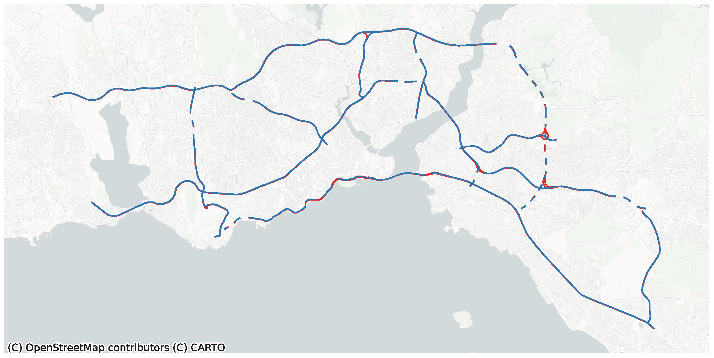
Segments are classified into two categories by their directions, while the ratio of major artery segments that have two directions is 88%, and the ratio of the major artery segments with only one direction is 12%. The major arteries of Istanbul are depicted in Figure 1, with the colors denoting their directions. As illustrated in the figure, the experiment region covers almost all areas of the Istanbul city. As a result of this variety, the dataset includes a wide range of traffic patterns and many anomalies like accidents, weather conditions, and sports or cultural events.

Figure 1. Major arteries of Istanbul.

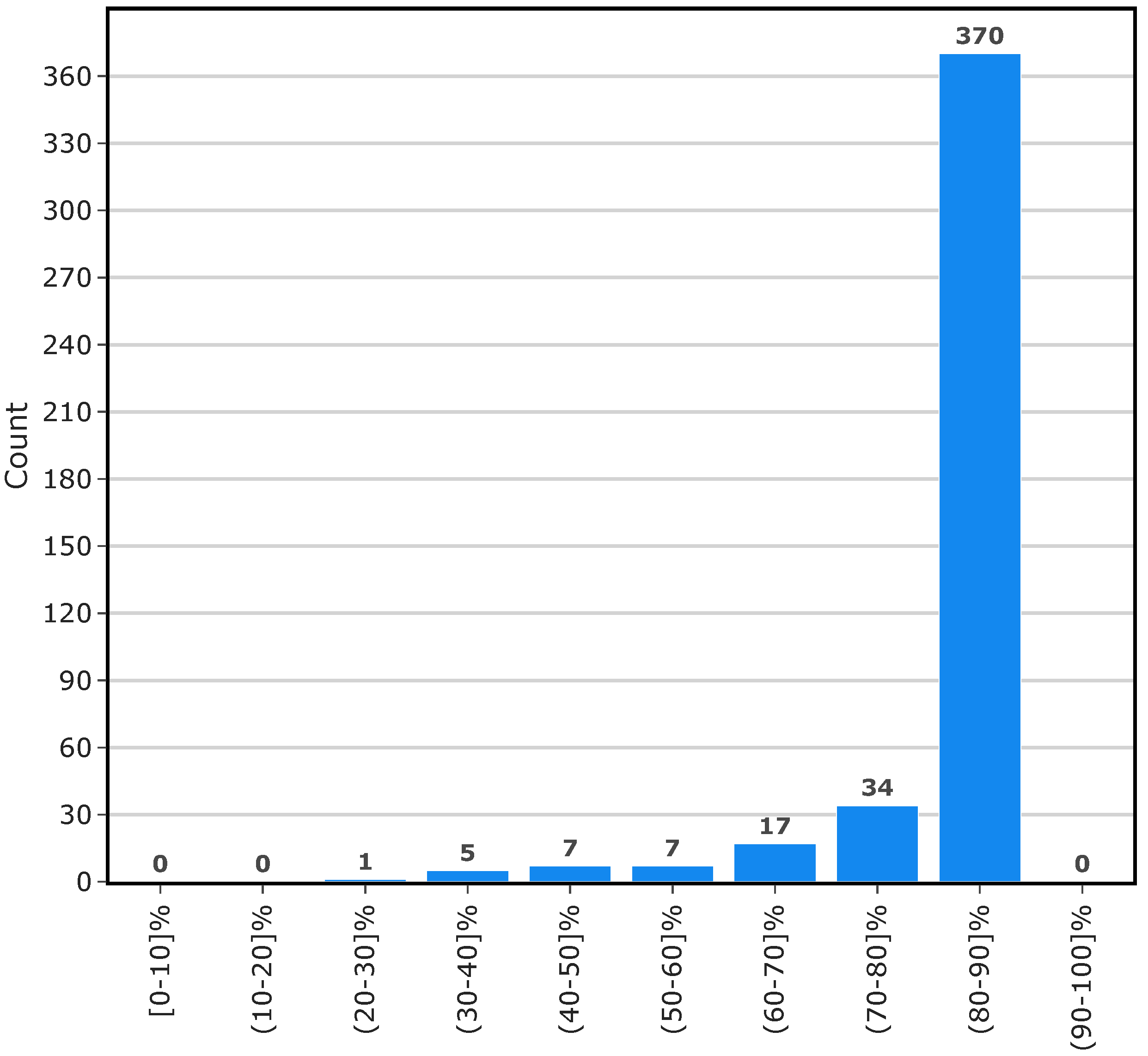
In its raw form, this dataset contains many missing values. To be able to understand the scale of the missing value problem, first, missing value ratios of 441 major segments are calculated for the year of 2018. Figure 2 displays the completeness ratios of the major segments before any preprocessing is performed.

Figure 2. Completeness ratios of major segments before preprocessing.

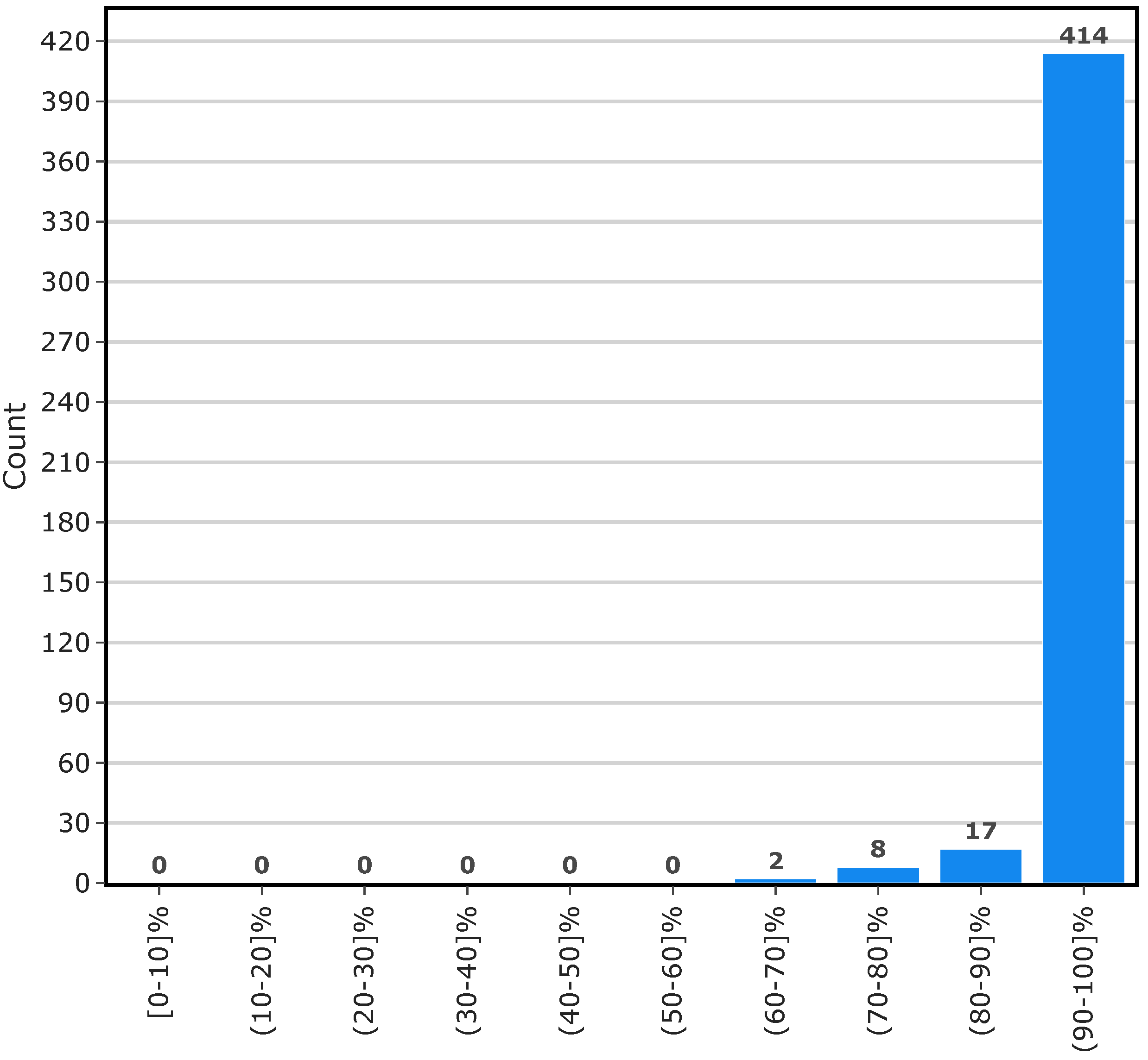
The chart reveals that many of the major segments actually have a low number of missing values. It is also observed that many of these missing values are non-consecutive, small gaps which can be easily closed while converting the resolution of the dataset from 1 min to 5 min using the sliding window approach. Nevertheless, even after this process, there were still some relatively long and consecutive gaps that remained. No further preprocessing was applied to remove these gaps since the number of these long gaps are negligible, and during testing these gaps are not predicted since it is not possible to compare them against ground truth values. Figure 3 displays the missing value ratios of the major segments after the 5 min sliding window preprocessing step.

Figure 3. Completeness ratios of major segments after preprocessing.

3.2. California Department of Transportation—PeMS Dataset

Experiments on the PeMS dataset are also conducted to ensure the reproducibility and verifiability of the experiments in this research [44]. Access to the traffic data archives of California was gained by contacting the California Department of Transportation. Traffic data from District 8 for the years 2017, 2018, and 2019 were then downloaded. Although predictions will only be made for 2018, data from the previous year are needed for training purposes since past months are used in the training. To be able to compare the predictions made for the last time steps of 2018 with the ground truth values, the traffic data from the next year are also needed. After downloading the data, the following steps are applied to prepare the dataset for the experiments:

• The original PeMS dataset stores traffic values by the days they are collected in separate files. Since the dataset acquired from the Istanbul Metropolitan Municipality has separate files for each segment, the PeMS dataset is converted into the same structure to ease the training and testing processes.
• Stations that are not common in all three years are discarded and a total of 2084 stations were covered.
• Missing values are detected by evaluating the jumps in the timestamps and marking them with a special value, which is −1. Following this process, each station file is found to contain the same number of rows, amounting to 105,120, given that there are 105,120 5 min intervals in a year.
• Missing value ratios of stations are calculated and those whose missing value ratio is not between 0 and 1 for all three years are discarded from the dataset. Thus, the number of stations is reduced to 1365.
• To reduce experiment durations, 105 evenly spaced stations are chosen among the stations and ordered by their respective station ID.

4. Baseline Traffic Prediction Methods

In view of the demonstrated efficacy of RNNs in modeling time series data, this study exploits two RNN-based networks comparatively, namely, LSTM and GRU, which have been validated in the domain of traffic prediction. These networks are employed to incorporate short-term characteristics into the analysis. Conversely, for modeling long-term characteristics, the historical average (HA) method, which is a relatively straightforward yet effective algorithm, is utilized.

4.1. Historical Average

The concept behind the HA method is to forecast future outcomes by averaging the speed data obtained from the same hour and day of previous weeks. It usually produces acceptable results in terms of long-term prediction when applied to data with periodical aspects [45]. Thus, we came up with the idea to exploit distant historical data as new features by training short-/medium-term traffic forecasting.

The HA method defines predicted speed $V_{prediction}\left(t\right)$ by Equation (1) where $V_{ts}^w$ denotes the speed value that comes w weeks before the time to be predicted. k denotes how many previous weeks are used while making the prediction and i represents how many time steps before and after the time t to be predicted are included.

$$V_{prediction}\left(t\right)={\displaystyle \frac{1}{k(2i+1)}}\sum _{w=1}^k\sum _{ts=-i}^i{V}_{ts}^w$$

(1)

4.2. Long Short-Term Memory

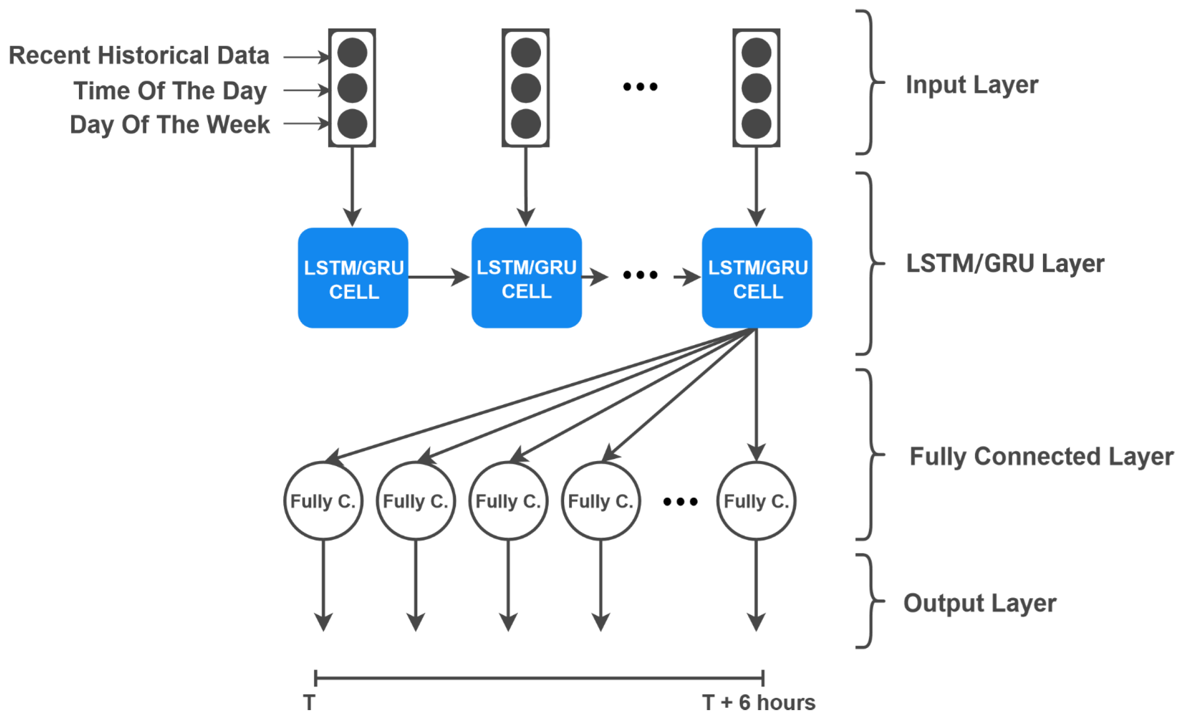
LSTM is a type of RNN that can learn and remember information over long periods of time. It uses memory cells which include forget, input, and output gates to store and alter the information flow. Thus, it can effectively handle sequential data such as time series and natural language. LSTMs are commonly used in tasks such as language translation, speech recognition, predicting future values of time series, and time series classification. There are also several studies [46,47,48] exploiting LSTM for short-term traffic prediction. Using recent historical data is a common practice in the literature when making predictions for short- and medium-term traffic speeds. A conventional model that employs LSTM or GRU units, which are fed by recent historical data, is illustrated in Figure 4. Recent historical data, time of the day, and day of the week are given in the input layer in order to get predictions up to 6 h. For an LSTM implementation LSTM cells are used to regulate the flow of information better.

Figure 4. Structure of LSTM- and GRU-based models.

4.3. Gated Recurrent Unit

GRU is a type of RNN, similar to the LSTM model. However, the GRU model uses fewer parameters due to the fact that it does not have an output gate. This allows the model to be larger or trained faster while achieving similar results to the LSTM models. Therefore, they can be used interchangeably with LSTM models. Depending on the context and conditions, they can also outperform the LSTM models since they have fewer parameters and hence are less prone to over-fitting.

5. Fusing Distant and Recent Historical Data

To utilize the strengths of distant and recent historical speed values both, a hybrid model which combines the historical average method and an RNN-based model is developed. Unlike the typical strategy of changing the model structure in the literature, two novel models, H-LSTM and H-GRU networks, were designed primarily based on the enrichment of the input data to improve short-/medium-term forecasting results. In this proposed approach, distant and recent historical values were fed together into the model where the distant and recent historical values are defined as follows:

• Recent Historical Data: Data that are not historically distant from the prediction period and are placed in the near past in terms of minutes. They can be useful to determine the fluctuations from the main characteristics of the time range to be estimated since they involve the information about just before the ground truth values.
• Distant Historical Data: In this paper, the average speed values of the previous 1 to 6 weeks respective to the time to be estimated are utilized as distant historical data. Unlike the recent historical data, distant historical data contain historical data of the same time range with the ground truth values, making them useful for learning speed changes that are recurring throughout consecutive weeks.

5.1. Model Structure

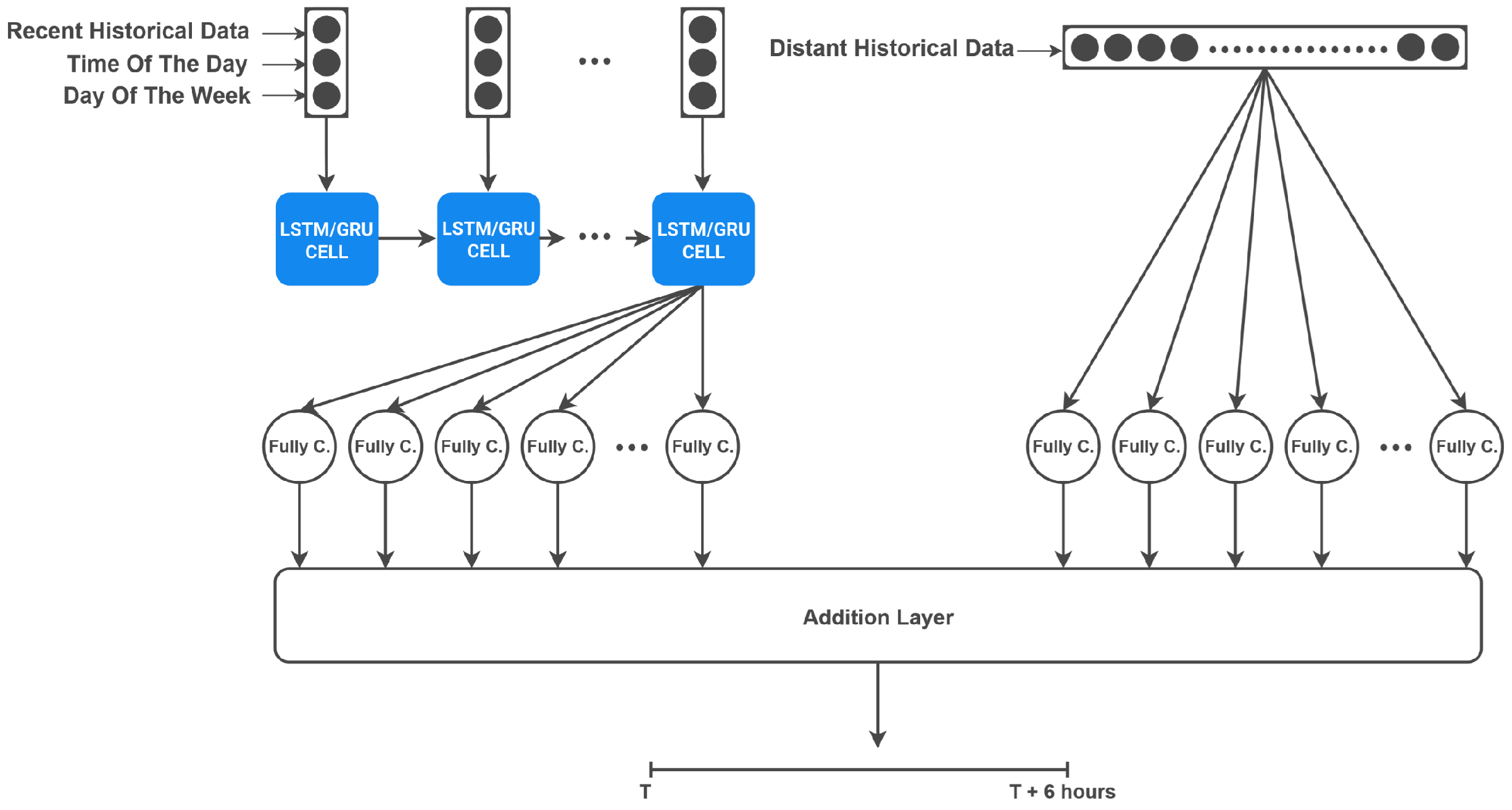
The structure of the proposed model is shown in Figure 5 where the left part is responsible for processing the recent historical data and the right part has the fully connected layer which takes distant historical data as input. In the model structure, the processing of recent historical data is conducted using one of the RNN-based networks, LSTM or GRU, and a fully connected layer, while the distant historical data are processed using a fully connected layer. The results from both parts are then merged together in an addition layer to create the output layer of the model.

Figure 5. The main structure of the proposed H-LSTM and H-GRU models.

As demonstrated in Figure 4 and Figure 5, the main difference of the proposed H-LSTM and H-GRU models from baseline models is that they are fed with distant historical data in addition to recent historical data.

5.2. Proposed Network Feeding Strategy for Distant and Recent Historical Data

H-LSTM and H-GRU models have two input layers. The first of these layers is the recent historical data. Equation (2) shows the notation and mathematical representation of recent historical data: $D_{recent}$, where $V_{current}\left(t\right)$ denotes the speed value that comes t minutes before the time range to be predicted.

$$\begin{array}{c}\overrightarrow{D_{recent}}={\left[V_{current}{\left(t\right)}_i\right]}_{i=1}^n\mathrm{where}\mathrm{t}=-40,-35,\dots ,0,\mathrm{n}=9\end{array}$$

(2)

$$\overrightarrow{D_{distant}}={\left[V_{prediction}{\left(t\right)}_i\right]}_{i=1}^n\mathrm{where}\mathrm{t}=5,10,\dots ,360,\mathrm{n}=72$$

(3)

To increase the prediction accuracy, time of the day and day of the week information of recent historical values are also added as a part of the first input layer. The second input layer takes the distant historical data. Equation (3) shows the calculation process, where t represents how many timestamps are evaluated along the prediction horizon. The output of the historical average method, which is frequently used in time series prediction, constitutes the data that is used in the second input layer. This structure gives the proposed method its name since the model uses the output of the historical average method as input.

In the developed H-LSTM and H-GRU systems, sensor-specific models are trained, and each road segment provides internally consistent speed data. Although historical averages are incorporated into the training process, each training sample contains speed values from the same hour of the day. Because these values share the same temporal and contextual characteristics, their scale and distribution remain consistent. Therefore, no additional normalization is performed for these historical features.

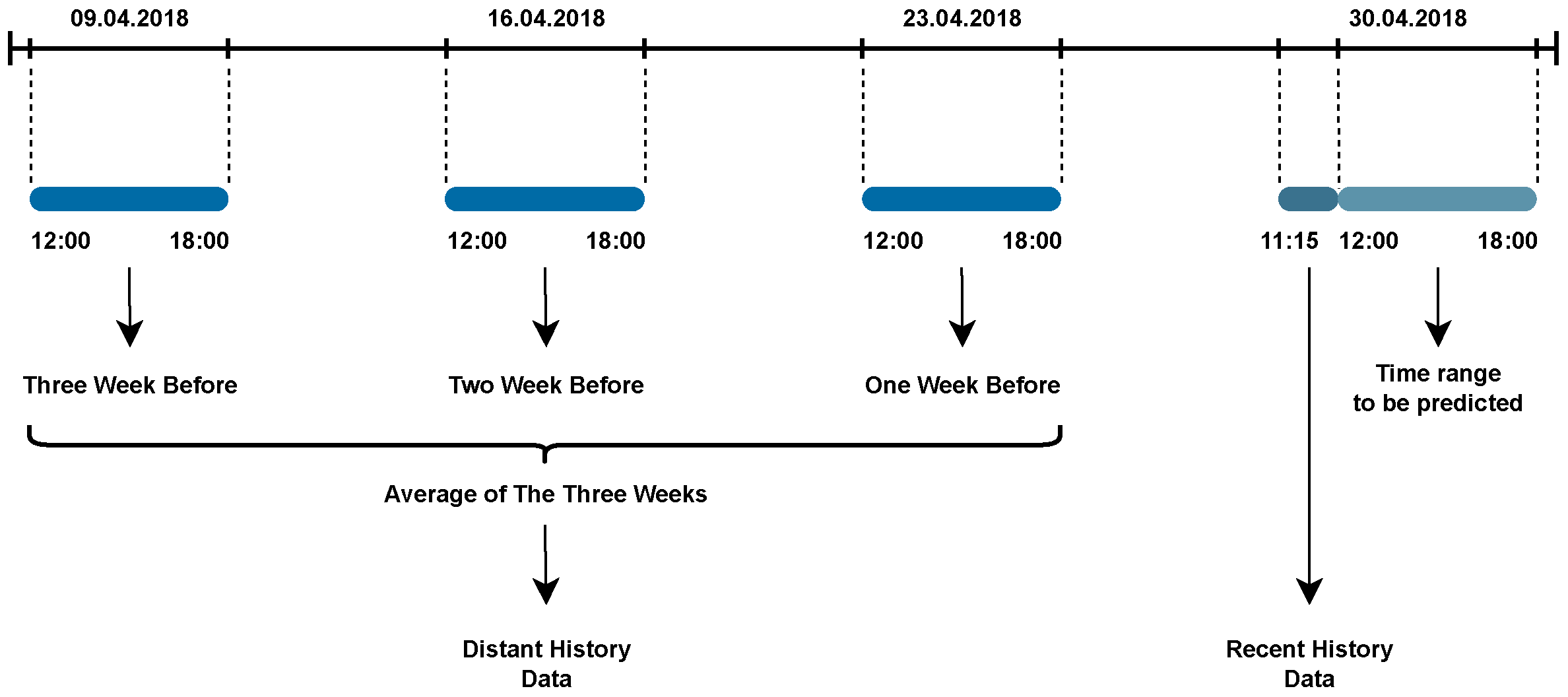
Figure 6 gives an overview about the usage of recent and distant historical data. In Figure 6, the average speed values of the three weeks preceding the time range to be predicted are used as distant historical data. Distant historical data contain values for the same time range as the time range to be predicted. In this example, that corresponds to the hours between 12:00 and 18:00. In order to make a clearer presentation of our algorithm, we provide the pseudocode of Algorithm 1.

Algorithm 1 Data Preparation and Model Input Generation
Require: Time series dataset $\mathcal{X}$, Target start time t, Target duration $T_{pred}$
1:	Hyperparameters:
2:	$N_{weeks}\leftarrow 3$	# Number of previous weeks for Distant History
3:	$T_{recent}\leftarrow 45\min$	# Duration for Recent History
4:	$T_{week}\leftarrow 1\mathrm{week}$
	Distant History Calculation
5	${\mathbf{Sum}}_{vec}\leftarrow \mathbf{0}$	# Initialize sum vector with zeros
6	for $i\leftarrow 1$ to $N_{weeks}$ do
7:	$t_{start}^{\left(i\right)}\leftarrow t-(i\times T_{week})$
8:	$t_{end}^{\left(i\right)}\leftarrow t_{start}^{\left(i\right)}+T_{pred}$
9:	$V^{\left(i\right)}\leftarrow \mathcal{X}[t_{start}^{\left(i\right)}:t_{end}^{\left(i\right)}]$	# Get vector for week i
10:	${\mathbf{Sum}}_{vec}\leftarrow {\mathbf{Sum}}_{vec}+V^{\left(i\right)}$	# Accumulate values
11:	end for
12:	${\mathbf{D}}_{distant}\leftarrow {\mathbf{Sum}}_{vec}/N_{weeks}$	# Calculate average
	Recent History Calculation
13:	${\mathbf{D}}_{recent}\leftarrow \mathcal{X}[t-T_{recent}:t]$	# Get data immediately preceding target
	Model Prediction
14:	$\widehat{y}\leftarrow \mathrm{RNN}({\mathbf{D}}_{distant},{\mathbf{D}}_{recent})$
15:	return $\widehat{y}$

Figure 6. An overview of our feeding strategy for H-LSTM and H-GRU models.

6. Experimental Results

In this section, we first give the results of the hyperparameter optimization tests. We then present the test results of the proposed strategy regarding different forecast horizons. The predictions were made for the 441 segments throughout 2018. We focused mainly on the H-LSTM model, which is the best performing one among the others. We also analyze our results in terms of day hours and weekdays. We finally demonstrate how the results of H-LSTM outfits to the ground truth values.

We utilized both MAE (Mean Absolute Error) and MAPE (Mean Absolute Percentage Error), two well-known metrics that are often used in traffic forecasting, in order to evaluate the performance of the existing and proposed models. MAE and MAPE values are calculated by Equations (4)–(6) where $y_t$ denotes the ground truth value at the time point t and ${\widehat{y}}_t$ denotes the predicted value for the same time point.

$$e_t=y_t-{\widehat{y}}_t$$

(4)

$$MAE={\displaystyle \frac{1}{n}}\sum _{t=1}^n\left|e_t\right|$$

(5)

$$MAPE={\displaystyle \frac{100}{n}}\sum _{t=1}^n|{\displaystyle \frac{e_t}{y_t}}|$$

(6)

6.1. Hyperparameter Optimization

The proposed H-LSTM method has hyperparameters of the underlying base LSTM structure such as batch size and the number of LSTM cells as well as the hyperparameters originating from the mechanisms that are used to exploit distant historical data. To optimize the hyperparameters of the H-LSTM method, a series of experiments were carried out on a smaller group from the 441 segments that represent the original dataset. This is achieved by manually selecting 20 segments distributed around Istanbul with a standard deviation close to the original 441 segments.

The main hyperparameters specific to our methodology are described as follows.

• Window length of recent historical values: It represents how much recent historical data are utilized for traffic speed estimation.
• Number of weeks for distant historical values: It denotes how many of the previous weeks’ speed data will be averaged.
• Training Set Length (in terms of months) It determines how many of the previous consecutive months will be used during training to produce predictions for the following month.

First, the experiments were performed on 20 selected segments to determine the window length of recent historical values; while executing the experiments, training set length was set to 6 months and the average speed values of 4 previous weeks were used as distant historical input. The forecast horizon was determined as 360 min. The error rates of experiments for the window length of recent historical speeds are given in Table 1. Table 1 shows that using a window length of 45 min gave the lowest MAPE and MAE values. Afterwards, the experiments for training set length were conducted using the 45 min recent historical values, whereas the average speed values of 4 previous weeks were utilized as distant historical values. The error rates arising from experiments for training set length are given in Table 2 where the results indicate using the previous six months for training yields the lowest MAPE and MAE values.

Table 1. The effect of recent historical data length.

Window Length (Minute)	MAPE	MAE
25	13.93	7.66
45	13.81	7.59
90	14.12	7.81

Table 2. The effect of training set length.

Training Set Length (Month)	MAPE	MAE
2	14.40	7.97
4	14.07	7.71
6	13.81	7.59

Finally, experiments for determining the length of distant historical values were conducted; while executing the experiments, the window size was chosen as 45 min and the training set length was set to 6 months. Table 3 gives the error rates of experiments for determining the number of weeks to average for distant historical values. Although prediction errors are very close to each other, using 3 weeks of distant historical values results in the lowest MAPE and MAE.

Table 3. The effect of the length of distant historical data.

Number of Weeks	MAPE	MAE
2	13.837	7.57
3	13.787	7.58
4	13.812	7.59
5	13.796	7.60
6	13.883	7.63

6.2. Performance of H-LSTM

In this section, traffic speed predictions for all 441 segments of Istanbul throughout the span of 2018 have been produced using the proposed H-LSTM model. All the results were obtained regarding the parameters given in Table 4. We also discuss the outcome derived from both temporal and spatial analyses.

Table 4. Hyperparameters of the H-LSTM model.

Hyperparameter	Value
Number of cells in the LSTM layer	200 cells
Number of units in fully connected layers	72 neuron
Epoch count	200 epoch
Batch size	512 sample
Early stopping criteria	25 epoch
Forecast horizon	5 min to 6 h
Duration of training set	6 month
Test set	1 month × 12
Window length of recent historical values	45 min
Number of weeks for distant historical values	3 weeks

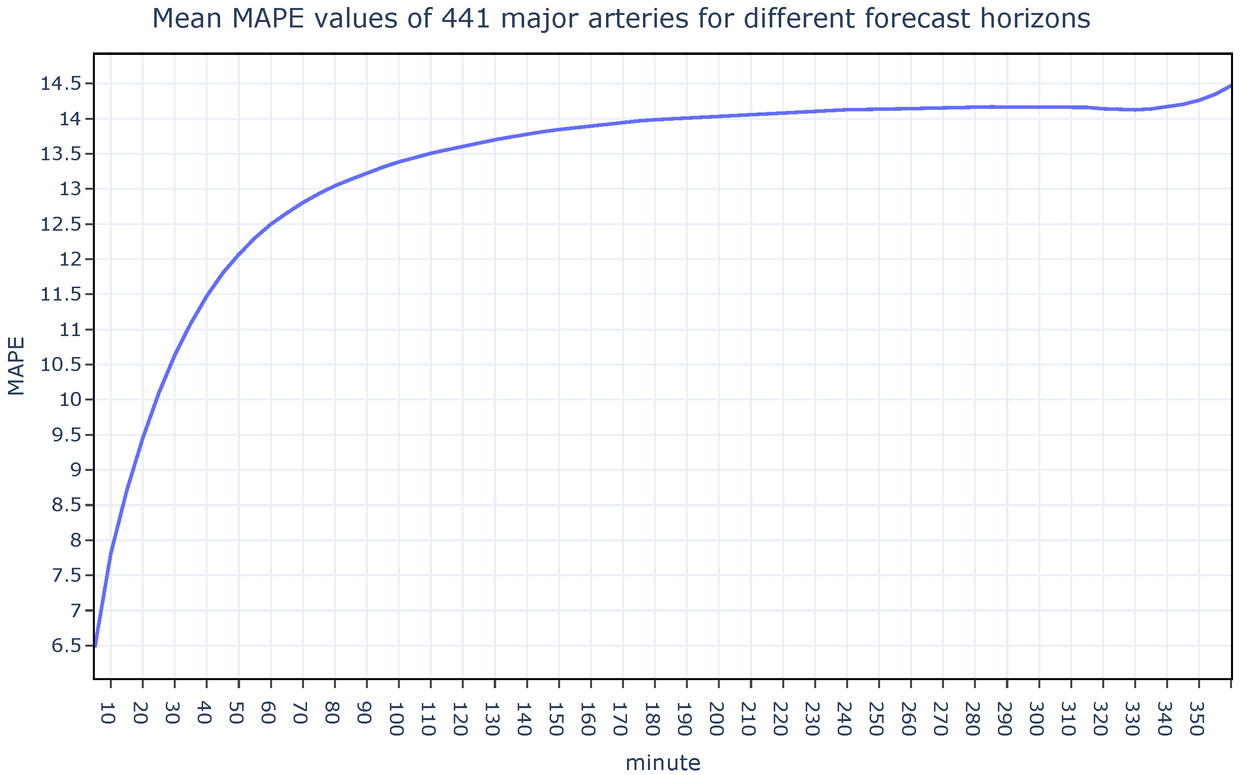
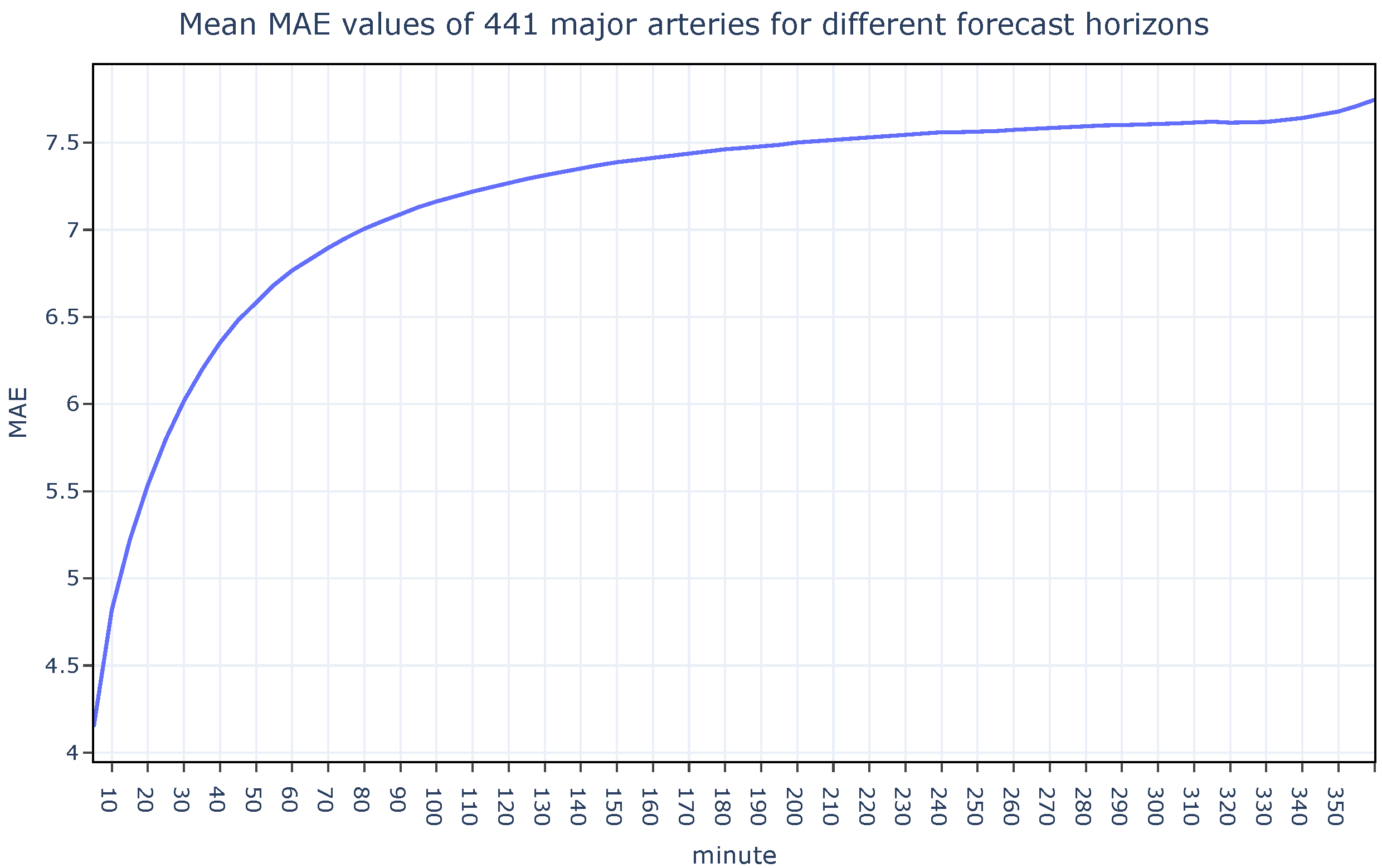
In the developed traffic forecasting system, traffic speed was predicted at every time point in the dataset for forecast horizons ranging from 5 to 360 min. During the experiments, the training window size was fixed at 6 months. For each test point, only the data preceding that point specifically, the previous 6 months, were used for model training. This rolling-origin evaluation strategy ensures that all test intervals are strictly isolated from the training data, preventing any information leakage from the future into the model. Figure 7 and Figure 8 show how the MAPE and MAE metrics change by forecast horizon. Instead of analyzing each segment on its own, the average MAPE and MAE values of all segments were illustrated. It is noteworthy that while error metrics are rising quickly up to 90 min, they begin to rise in the slow lane beyond that horizon forecast.

Figure 7. The MAPE values for all segments obtained by H-LSTM for varying forecast horizons.

Figure 8. The MAE values for all segments obtained by H-LSTM for varying forecast horizons.

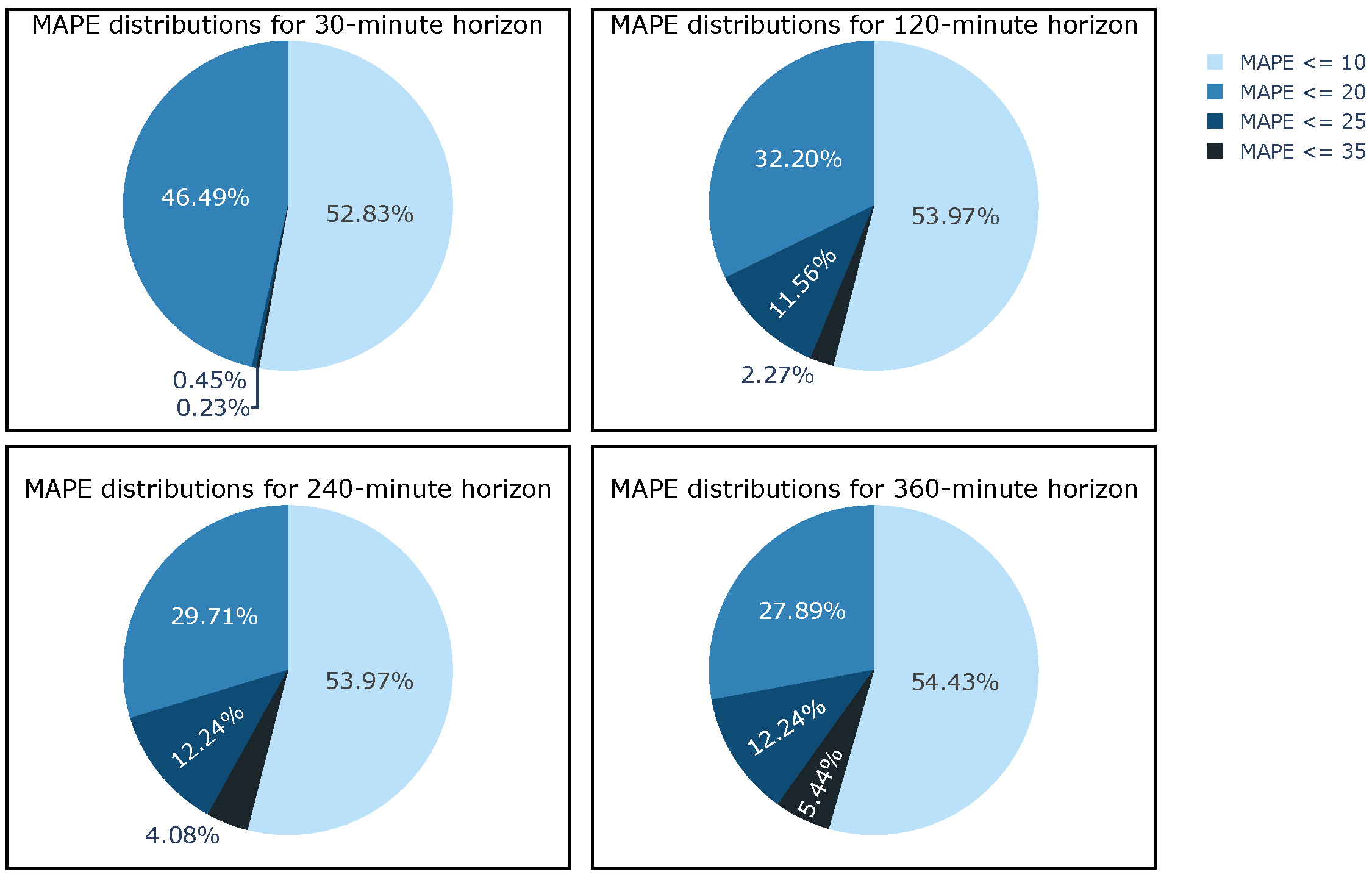
Considering the success of the studies on traffic flow prediction, segments with MAPE values below 10% can be accepted as very good predictions while those with MAPE values between 10% and 20% can be considered as acceptable. It is important to find which segments exceed these limits in order to identify problematic routes and areas prone to congestion. The MAPE distributions of the segments for the forecast horizons of 30, 120, 240, and 360 are shown in Figure 9. It is clear from the plots that as the forecast horizon increases, the number of segments whose MAPE value is under 10% decreases. For the predictions that are made with a 360 min forecast horizon, 27.9% of all the segments have MAPE values under 10%. Analyzing the overall results shows us that some segments already had MAPE values greater than 20% even at the 30 min forecast horizon. The principal reason for this outcome may be attributed to the elevated annual accident rate or the greater density of vehicles observed in these segments in comparison to other segments. Nevertheless, since the number of these segments is quite low, it can be concluded that the proposed H-LSTM model produces satisfactory results for a real-world scenario.

Figure 9. MAPE distributions of 441 major segments obtained by H-LSTM.

We also analyzed the performance of H-LSTM regarding the 6 h zones of the day. Table 5 shows the average prediction results for the hours of 00:00, 06:00, 12:00, and 18:00. The graphs demonstrated that predictions made throughout the night have lower MAPE and MAE values than those made during the evening and afternoon. This fact can be attributed to the distinctive characteristics of rush hour. On the other hand, MAE values even for the longest forecast horizon, i.e., 6 h further, could be principally accepted for production. It is a fact that traffic flow characteristics may vary with the days of the week. Table 6 shows the average prediction results from Monday to Sunday. With the exception of Friday, most weekdays have similar error rates. This can be a result of Friday being the last weekday and thus having a different speed characteristic from other weekdays. It is clear that predictions made at weekend have lower error rates than estimation values on workdays, since usually there are no specific rush hours on weekends, especially on Sundays.

Table 5. The performance of H-LSTM regarding the forecast horizon and daytime.

	30 min Horizon		120 min Horizon		240 min Horizon		360 min Horizon
Hours	MAE	MAPE	MAE	MAPE	MAE	MAPE	MAE	MAPE
00:00	4.92	6.70	5.42	6.52	5.66	6.75	5.30	6.60
06:00	5.48	7.77	8.42	17.58	7.94	15.50	7.78	15.12
12:00	6.17	11.52	8.14	16.26	9.57	20.15	10.75	26.43
18:00	7.73	19.38	8.59	17.55	6.18	10.33	6.29	9.76
Average	6.08	11.35	7.65	14.48	7.34	13.19	7.53	14.48

Table 6. The performance of H-LSTM regarding the weekdays.

	30 min Horizon		120 min Horizon		240 min Horizon		360 min Horizon
Day of the Week	MAE	MAPE	MAE	MAPE	MAE	MAPE	MAE	MAPE
Monday	6.00	10.50	7.20	13.30	7.47	13.68	7.57	13.68
Tuesday	6.07	10.91	7.29	13.82	7.53	14.20	7.64	14.34
Wednesday	6.06	10.92	7.25	13.76	7.47	14.15	7.62	14.40
Thursday	6.10	11.05	7.40	14.11	7.70	14.67	7.88	14.99
Friday	6.38	11.82	7.70	15.15	7.91	15.53	7.96	15.75
Saturday	5.87	10.34	7.22	13.66	7.55	14.30	7.85	14.93
Sunday	5.61	8.92	6.79	11.46	7.26	12.34	7.68	13.22
Average	6.01	10.64	7.26	13.61	7.56	14.12	7.74	14.47

6.3. Performance Comparison of Different Models

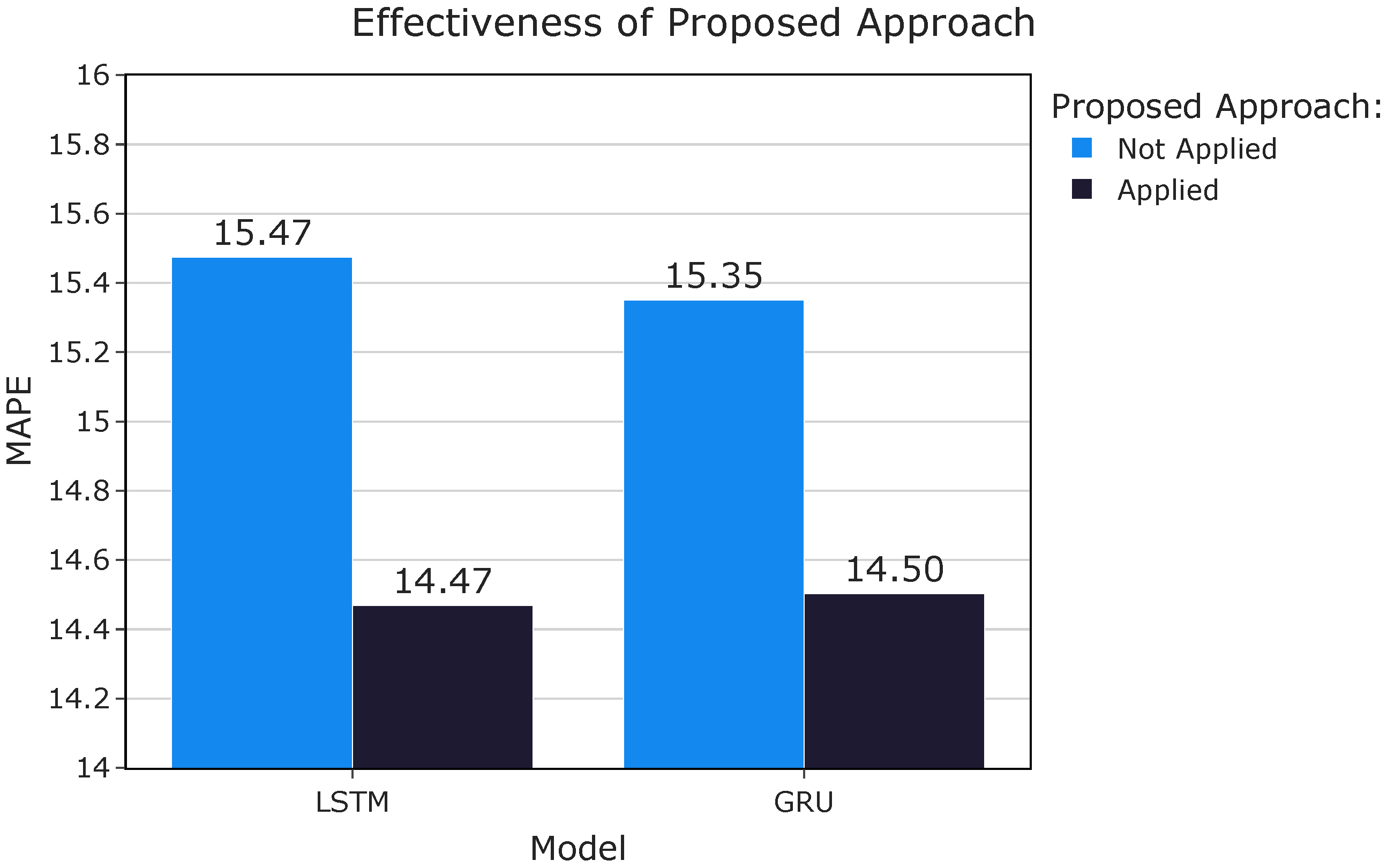
In order to evaluate the effect of fusing distant and recent historical data on prediction of short- and medium-term traffic prediction performance, changes in error metrics when the proposed approach is applied for both LSTM and GRU models are shown in Figure 10. The results demonstrate that our approach is not only limited to the LSTM and can be used with different model structures.

Figure 10. Effectiveness of proposed approach on different model types.

Analyzing the results it is observed that H-LSTM outperforms other methods on the dataset we acquired from the Istanbul Metropolitan Municipality. To assess the efficacy of the proposed method in forecasting outcomes across varying forecast horizons and time of day, further tests were conducted to compare the performance of H-LSTM, LSTM, and the historical average.

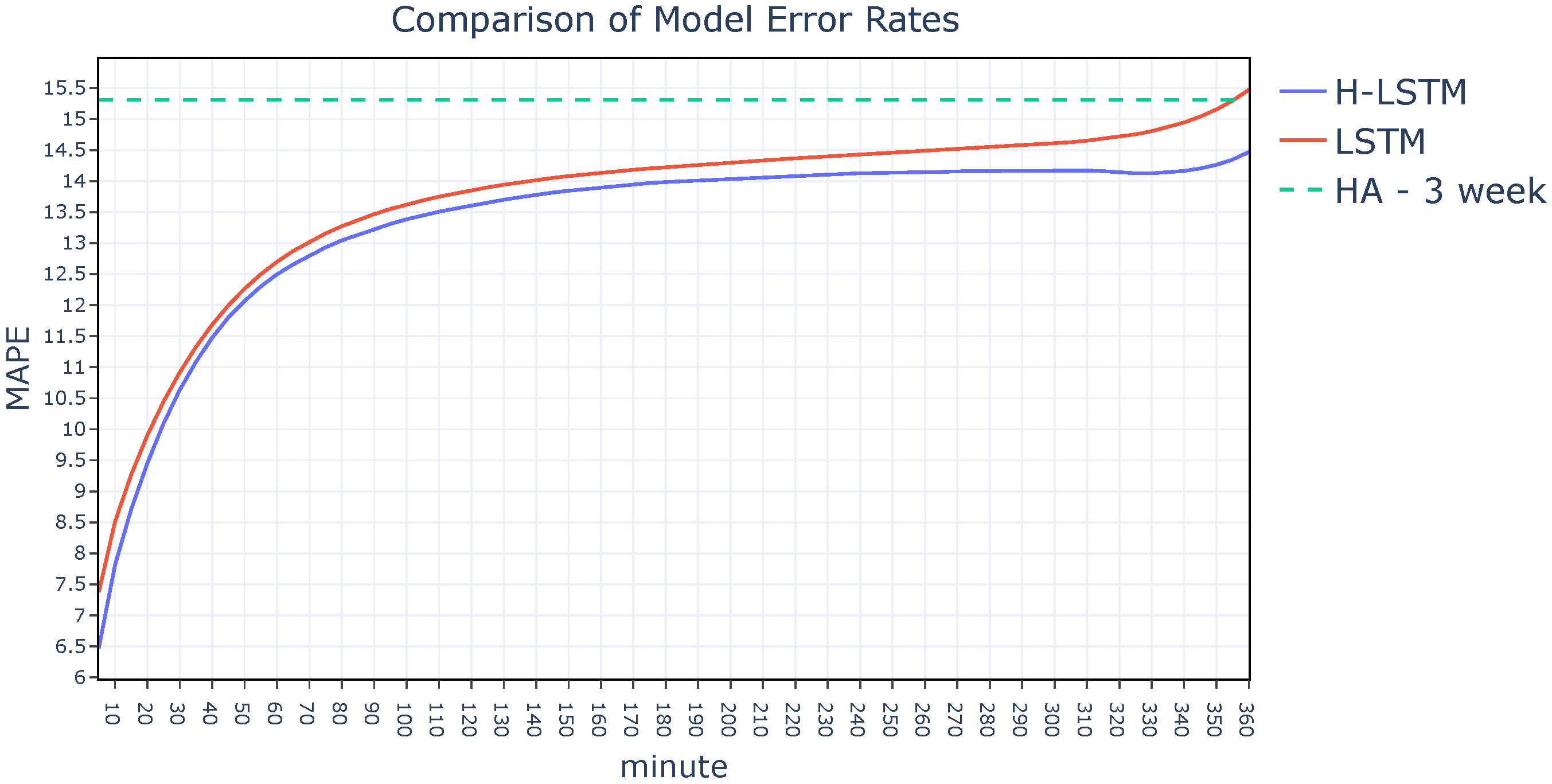
Figure 11 shows how the MAPE value changes with the forecast horizon. Since the historical average method directly takes averages from prior time periods to produce predictions, the forecast horizon has negligible impact on its error rate, so it is important to note that the average performance for the whole year is given in respective Figures to obtain a clean representation. The plot shows that the H-LSTM model outperforms both the HA model and the LSTM model in terms of accuracy. As the forecast horizon gets longer, the differences between the models become even more apparent. Thus, it can be claimed that the reason the H-LSTM model gives more accurate findings towards the longer forecast horizons is that it utilizes distant historical data as well.

Figure 11. Comparison of model error rates by forecast horizon.

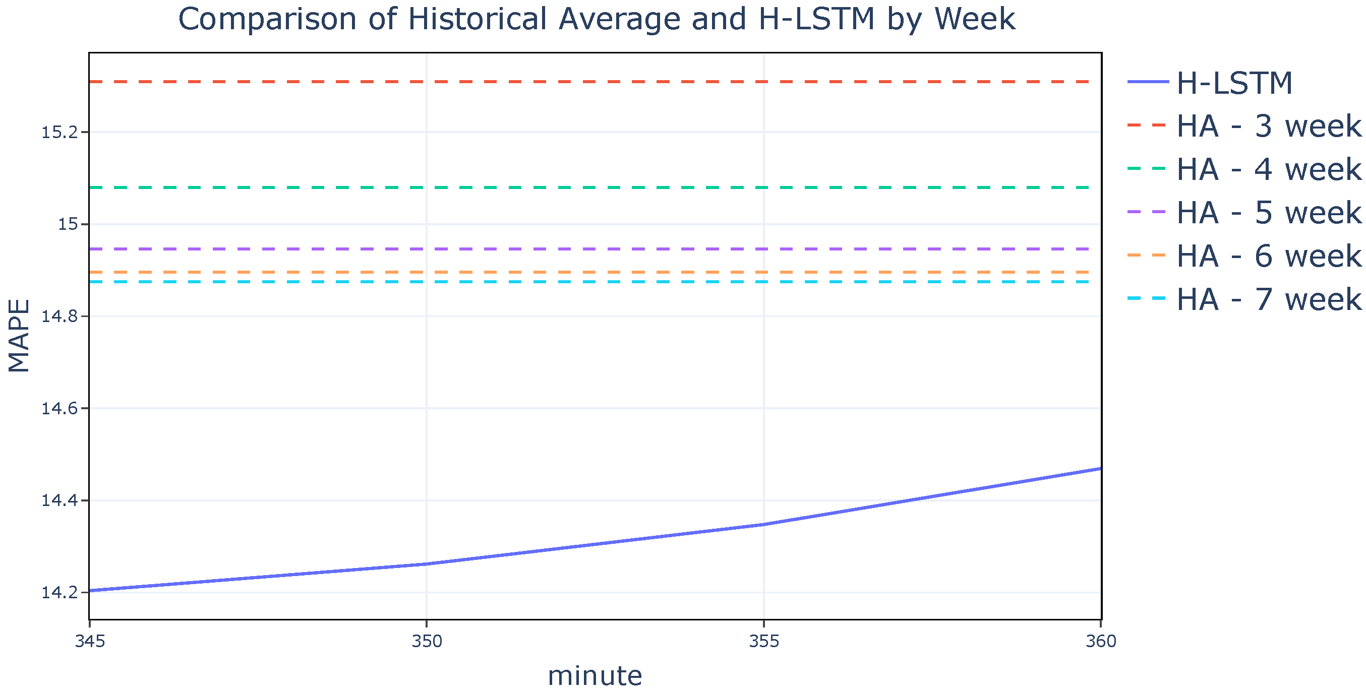
The effect of taking the mean for different numbers of previous weeks for the HA method is shown in Figure 12. The x-axis of the plot is limited to the range between 345 and 360 min horizons to display the difference between the results of the historical average method more clearly.

Figure 12. The effect of number of weeks for HA method.

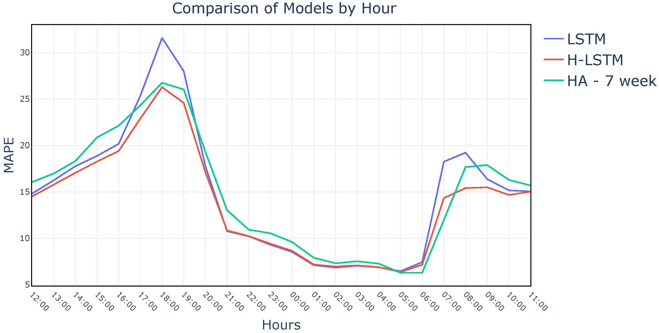
As provided in the hyperparameter optimization section, the number to calculate the average speed of previous weeks is chosen as 3 for the H-LSTM model. Nevertheless, it is clear from Figure 12 that even after 3 weeks, the historical average method’s MAPE value gets slightly lower up to a point as the number of weeks increases. This proves that the usage of distant historical data is not the only factor helping H-LSTM perform better than LSTM. Instead, it shows that distant and recent historical data both contribute to producing more accurate results. Looking at the global average of the results will only provide a broad idea about their success. Therefore, the results are compared by the time of the day to find out which models make better predictions for particular hours. Figure 13 shows the comparison of the three models for medium-term predictions, i.e., 6 h in the future. It is clear from the plot that the H-LSTM model makes more accurate predictions by taking the powerful features of both input models. This shows that by using both distant and recent historical data together, the H-LSTM model was able to make predictions that are not possible to make by using only one of the input types.

Figure 13. Hourly performance comparison of models.

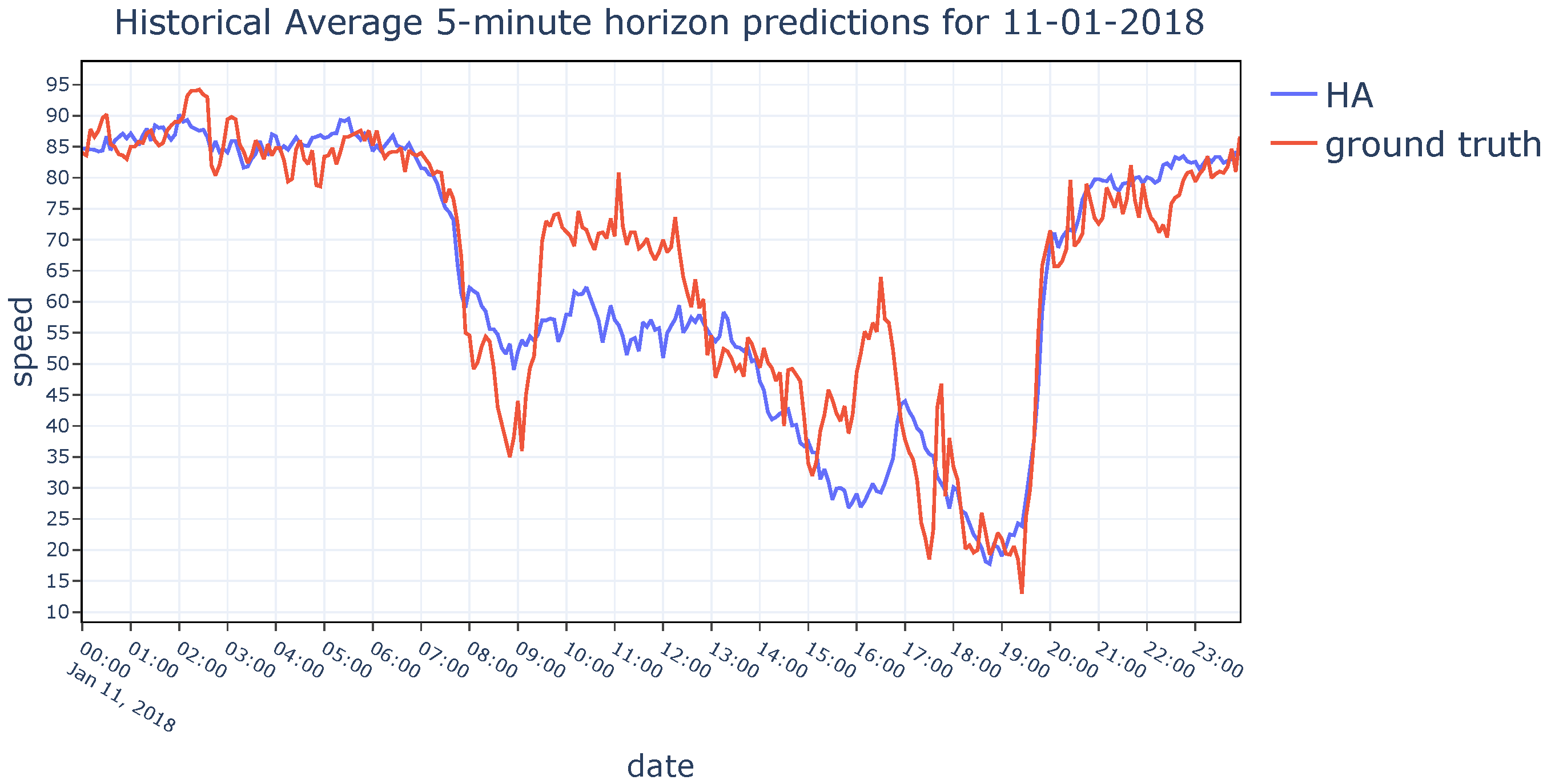
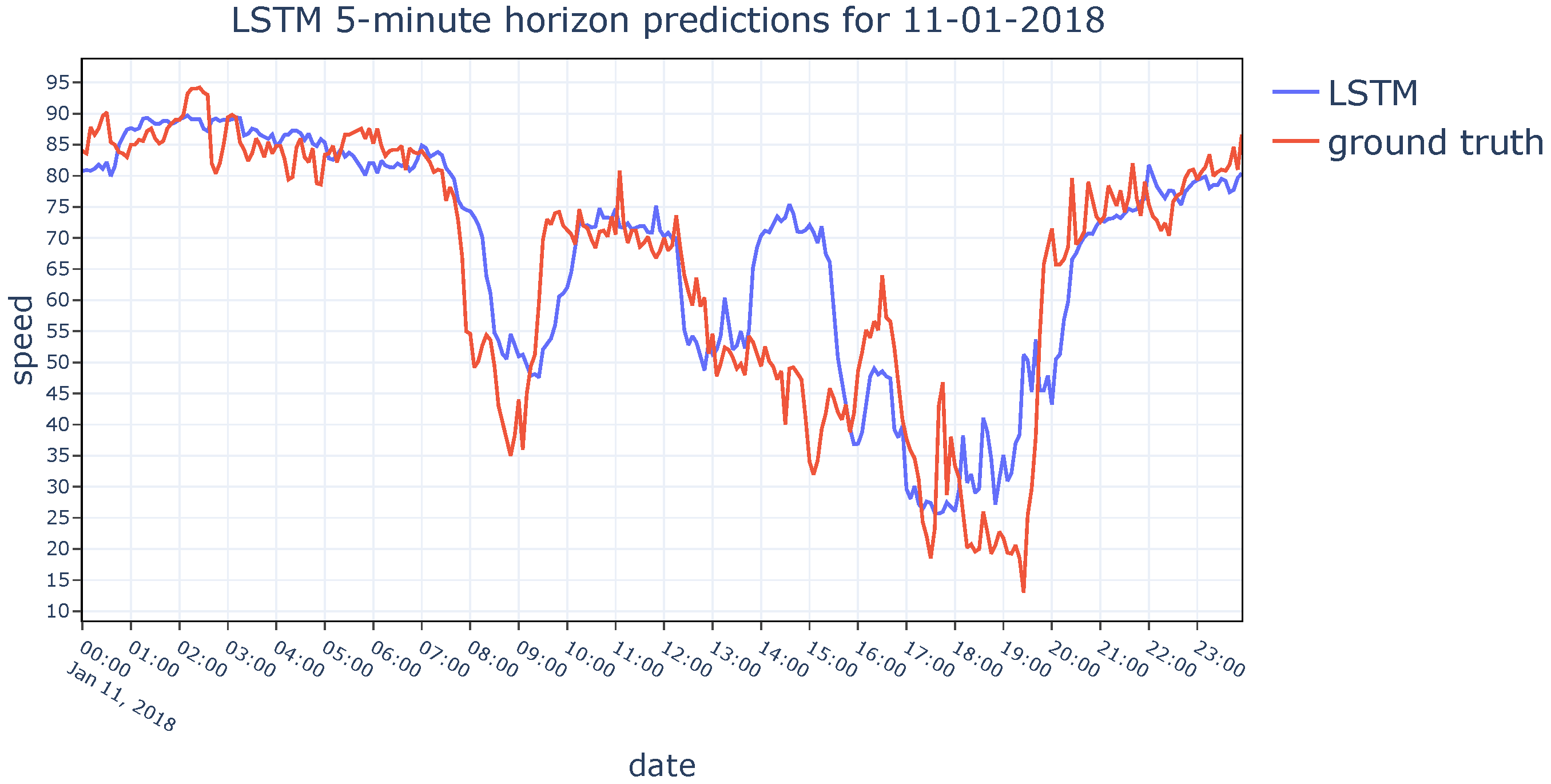
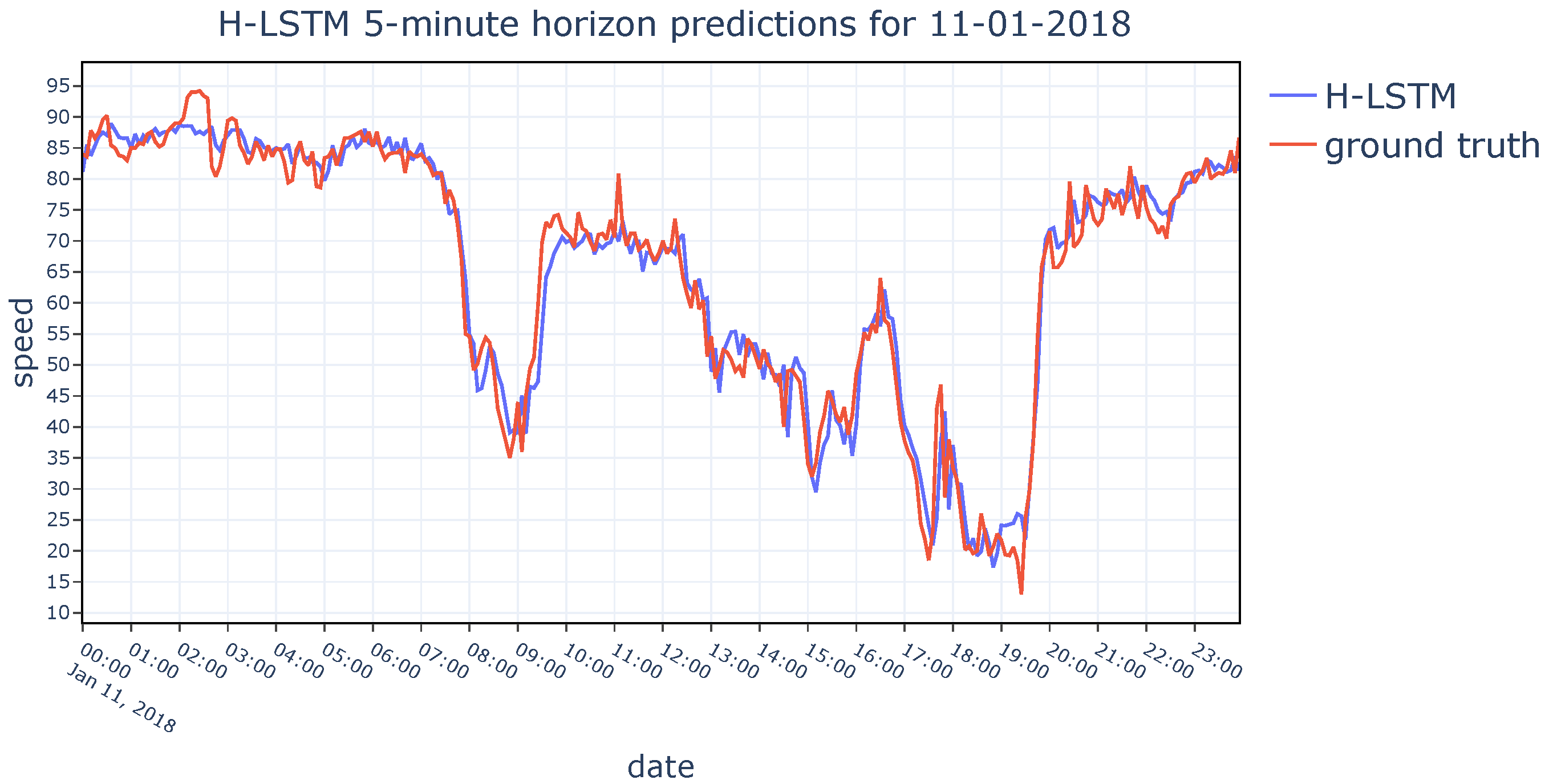
In order to provide a detailed analysis regarding the performance of the models, ground truth values from the dataset are compared with the results obtained by the three models. Predictions of the HA, LSTM, and H-LSTM methods for a randomly chosen day from the dataset are given in Figure 14, Figure 15 and Figure 16, respectively. The behavioral pattern observed in Figure 13 is also apparent in Figure 14, Figure 15 and Figure 16, where the H-LSTM model gets along with ground truth values in a superior harmony compared to the HA model and the base LSTM model.

Figure 14. HA’s daily prediction performance on 11 January 2018.

Figure 15. LSTM’s daily prediction performance on 11 January 2018.

Figure 16. H-LSTM’s daily prediction performance on 11 January 2018.

Finally prediction errors of all models that developed for the Istanbul Metropolitan Municipality dataset are given in Table 7. Best scores for each column are marked with bold characters.

Table 7. Prediction errors of models over varying forecast horizons.

	30 min Horizon		120 min Horizon		240 min Horizon		360 min Horizon
Model	MAE	MAPE	MAE	MAPE	MAE	MAPE	MAE	MAPE
LSTM	6.02	10.92	7.31	13.85	7.64	14.42	8.00	15.47
H-LSTM	6.02	10.64	7.27	13.61	7.56	14.13	7.75	14.47
GRU	6.01	10.81	7.27	13.69	7.61	14.33	7.97	15.35
H-GRU	6.02	10.65	7.30	13.69	7.57	14.20	7.74	14.50
HA–7 W	7.91	14.88	7.91	14.88	7.91	14.88	7.91	14.88

6.4. Performance of the Proposed Model on PeMS Dataset

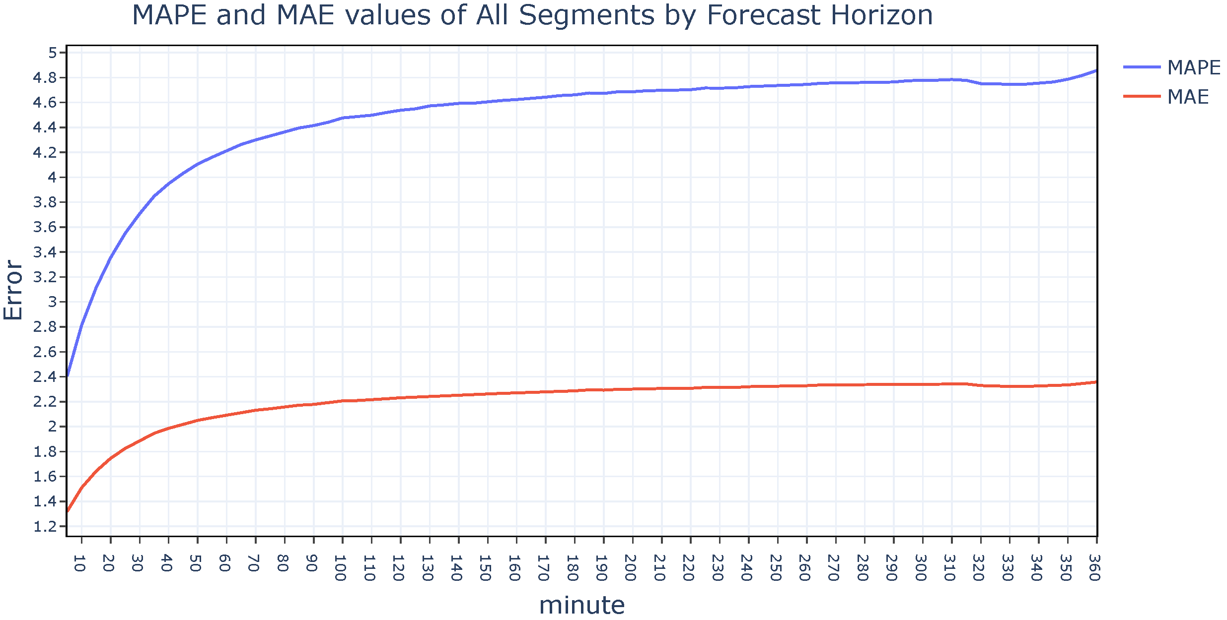
The results of the experiment conducted on the Istanbul dataset indicate that the H-LSTM model exhibited the most favorable performance. To gain further insight into the efficacy of the proposed method, we applied the H-LSTM model to the PeMS dataset. To make the experiments comparable, we used the same values for the hyperparameters of the experiments. Just as the previous experiments, experiments with the LSTM model and the historical average method are also conducted in order to compare H-LSTM results. We first give the MAPE and MAE averages of all segments compared to the forecast horizon in Figure 17.

Figure 17. The MAPE and MAE values obtained by employing the H-LSTM on all segments of the PeMS dataset, with varying forecast horizons.

Analyzing the results of experiments conducted on the PeMS dataset, we see the same patterns we observed for the Istanbul dataset. At the beginning both MAPE and MAE values are increasing faster and as the forecast horizons reach towards to end, the speed gets lower.

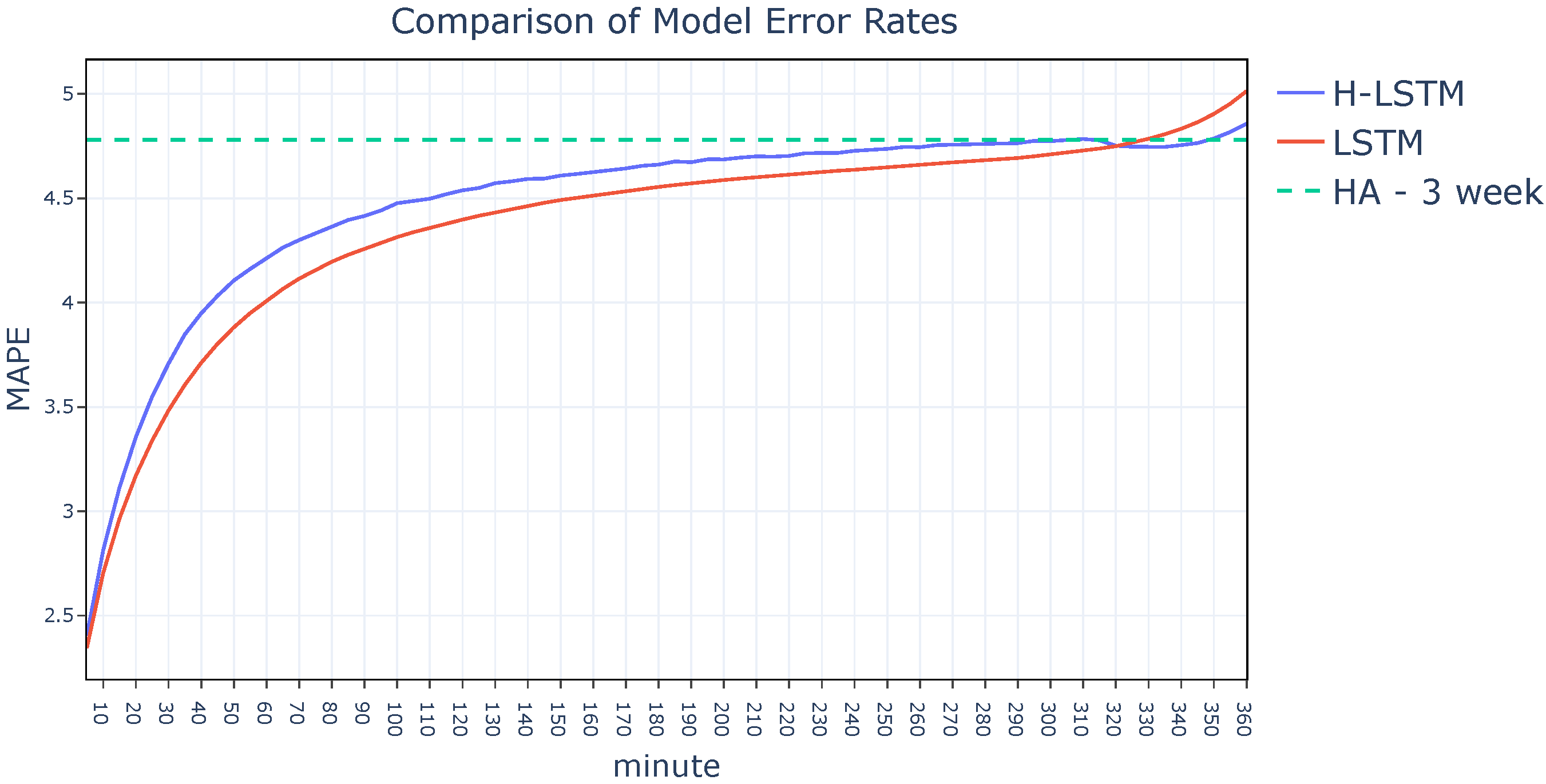
In order to reveal the effect of our proposed method, we compare H-LSTM results with results of the LSTM model and the historical average method. Figure 18 displays the error rates of the models by forecast horizon.

Figure 18. Error rates of the H-LSTM, LSTM, and HA models across different forecast horizons on the PeMS dataset.

It can be seen from the figure that the error rates of the H-LSTM model become lower than the LSTM model around the 320 min mark. H-LSTM performs better than LSTM as the forecast horizon increases. A comparison of the Istanbul dataset experiments with the historical average method reveals a contrasting outcome. The results indicate that the historical average method is more effective than the H-LSTM model for making predictions with a 360 min forecast horizon. However for lower forecast horizons, the H-LSTM model performs much better compared to the historical average method. In considering the overall performance of the models, it becomes evident that as the error rates of the H-LSTM and LSTM models approach those of the historical average method, the H-LSTM model exhibits superior performance in comparison to the LSTM model. This is anticipated, as the H-LSTM model utilizes the outputs of the historical average method during the training process.

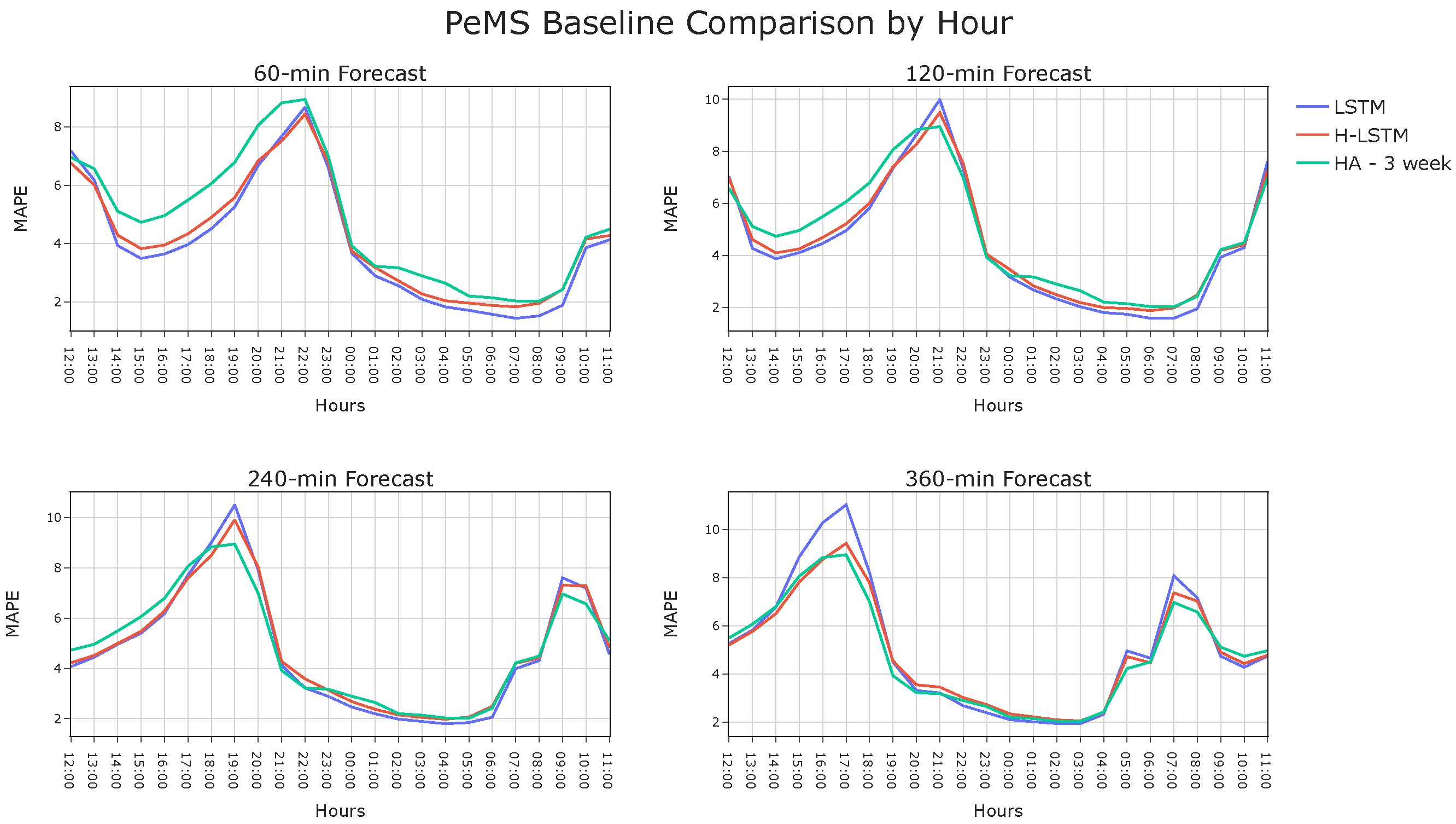
In order to provide a more comprehensive understanding of the models’ performance, an examination of the hourly prediction errors is conducted. The results of this examination are presented in Figure 19, which shows the hourly analysis for four different forecast horizons. For predictions with lower forecast horizons, H-LSTM model outperforms the historical average method by a significant margin, but it does not improve upon the LSTM model. Conversely, for predictions with higher forecast horizons, the H-LSTM model greatly outperforms the LSTM model, but it fails to perform better than the historical average method. Finally results of all the models we trained on the PeMS dataset can be seen in Table 8.

Figure 19. Performance of H-LSTM, LSTM, and HA methods on PeMS dataset which is provided on an hourly basis.

Table 8. Prediction errors of models.

	30 min Horizon		120 min Horizon		240 min Horizon		360 min Horizon
Model	MAE	MAPE	MAE	MAPE	MAE	MAPE	MAE	MAPE
LSTM	1.69	3.48	2.07	4.40	2.18	4.64	2.31	5.01
H-LSTM	1.89	3.71	2.23	4.54	2.32	4.73	2.36	4.86
HA–3 W	2.32	4.78	2.32	4.78	2.32	4.78	2.32	4.78

Performing hyperparameter optimization on the PeMS dataset might contribute to the success of the system. Another potential explanation for these findings is that the dynamic characteristics of the Istanbul dataset are more sophisticated than those of the PeMS, which may allow the H-LSTM method to perform better in long-term forecasting than other methods in the Istanbul dataset. Analyzing the PeMS dataset shows us that speed values of the Istanbul dataset have an uncertain characteristic compared to speed values in PeMS. These patterns in PeMS are easy to predict and so prediction errors are quite low. Thus, H-LSTM could only start to beat LSTM after 360 min in terms of MAPE. On the other hand, HA performs well for long-term traffic speed estimation where recent speed values start to subvert predictions. All test results demonstrated that a dynamic method that employs the model with the lowest error rate among H-LSTM, LSTM, and HA for different forecast horizons can be developed.

7. Discussion

As discussed in Section 5, distant historical data contain information about common patterns that are observed in the previous weeks, whereas recent historical data reflect short-term fluctuations that may arise from weather conditions, accidents, or cultural and sporting events. Although the present study uses only speed data without explicitly incorporating such contextual factors, it maintains broad applicability. Because it operates purely through time series manipulation, it can be applied to any speed dataset from any geographical region while still allowing the integration of contextual variables when available. Future work may extend this approach by incorporating contextual factors into both distant and recent historical representations.

The main strength of this proposed method lies in its ability to enhance prediction accuracy through input restructuring rather than through a complex model architecture. Distant historical data are constructed by averaging over past adjacent weeks for the same time interval, while cyclical traffic variations are represented through day-of-the-week and time-of-day features. This design enables the model to capture patterns such as increased Monday morning traffic that cannot typically be learned from recent data alone. Experimental results confirm that prediction performance remains stable across days of the week, indicating successful modeling of weekly cycles. The simplicity of this strategy distinguishes it from prior work focused on complex feature selection schemes and also allows it to be seamlessly combined with other input enhancement methods. Nonetheless, additional improvements could be achieved by incorporating traffic characteristics specific to national or religious holidays.

Although the method effectively leverages both recent and distant historical information, relying solely on historical data may not be sufficient to capture sudden deviations caused by unexpected events. Traffic conditions can change rapidly due to incidents, abrupt weather shifts, road closures, or route adjustments driven by navigation applications. Integrating real-time data into the system therefore represents a promising direction for improving adaptability in practical deployments. A hybrid approach—combining traditional road sensor data with real-time information from connected vehicles or navigation systems—could allow continuous correction of predictions. Such streaming data can be incorporated through online learning mechanisms to refine outputs in near real-time, particularly during irregular congestion events where historically driven models often underperform.

Finally, the optimal lengths for the training set, recent historical data, and distant historical data are determined empirically and then kept constant. Fixing these hyperparameters provides several benefits: the resulting framework remains simple, transparent, and computationally efficient, while avoiding the introduction of additional learnable parameters that could increase training complexity or increase the risk of overfitting. However, this strategy also has limitations. By assigning equal weight to all selected weeks, it cannot emphasize weeks that are more informative or downweight those affected by anomalies such as holidays or extreme weather. Moreover, the optimal hyperparameters may vary across cities, seasons, or road types, requiring manual tuning. Therefore, temporal weighting or attention-based mechanisms could automatically learn the most relevant historical periods, offering greater adaptability at the cost of increased model complexity.

8. Conclusions

In this study, the novel H-LSTM model is introduced for short- and medium-term traffic speed estimation. With the help of the proposed model, unlike the common approach of using only recent historical data when predicting traffic in the short and medium term in the literature, both recent historical data and distant historical data, which are the average speed values of previous weeks, are utilized. Since the proposed H-LSTM method exploits distant historical data by compromising LSTM and fully connected layers, it requires relatively low computational power. It is observed that the H-LSTM model makes up to 20% more accurate predictions compared to the traditional approach. All three of the models have been tested on 441 major arteries of Istanbul city, where 80% of the segments were predicted with lower than 20% MAPE with the help of H-LSTM regarding a forecast horizon of 6 h.

In future research, more complex and bigger models such as transformers or graph neural networks can be used to test if using recent and distant historical data together improves the accuracy in those types of models too. Furthermore, since the method we propose does not rely on any domain specific data or knowledge, it could also be used to predict different time series data domains.

References

1. Beland, L.P.; Brent, D.A. Traffic and crime. J. Public Econ. 2018, 160, 96–116. [Google Scholar] [CrossRef]
2. Sánchez González, S.; Bedoya-Maya, F.; Calatayud, A. Understanding the Effect of Traffic Congestion on Accidents Using Big Data. Sustainability 2021, 13, 7500. [Google Scholar] [CrossRef]
3. TomTom. Traffic Congestion Ranking: Tomtom Traffic Index. Internet Archive: Wayback Machine (archived 1 October 2022). Available online: https://web.archive.org/web/20221001012718/https://www.tomtom.com/traffic-index/ranking/ (accessed on 6 December 2025).
4. Liu, Q.; Wang, B.; Zhu, Y. Short-Term Traffic Speed Forecasting Based on Attention Convolutional Neural Network for Arterials. Comput.-Aided Civ. Infrastruct. Eng. 2018, 33, 999–1016. [Google Scholar] [CrossRef]
5. Guo, G.; Yuan, W. Short-term traffic speed forecasting based on graph attention temporal convolutional networks. Neurocomputing 2020, 410, 387–393. [Google Scholar] [CrossRef]
6. Liu, D.; Tang, L.; Shen, G.; Han, X. Traffic Speed Prediction: An Attention-Based Method. Sensors 2019, 19, 3836. [Google Scholar] [CrossRef] [PubMed]
7. Park, H.S.; Park, Y.W.; Kwon, O.H.; Park, S.H. Applying Clustered KNN Algorithm for Short-Term Travel Speed Prediction and Reduced Speed Detection on Urban Arterial Road Work Zones. J. Adv. Transp. 2022, 2022, 1107048. [Google Scholar] [CrossRef]
8. Wang, Y.; Li, L.; Xu, X. A piecewise hybrid of ARIMA and SVMs for short-term traffic flow prediction. In Proceedings of the International Conference on Neural Information Processing, Guangzhou, China, 14–18 November 2017; Springer: Cham, Switzerland, 2017; pp. 493–502. [Google Scholar]
9. Li, K.L.; Zhai, C.J.; Xu, J.M. Short-term traffic flow prediction using a methodology based on ARIMA and RBF-ANN. In Proceedings of the 2017 Chinese Automation Congress (CAC), Jinan, China, 20–22 October 2017; pp. 2804–2807. [Google Scholar] [CrossRef]
10. Kumar, S.V.; Vanajakshi, L. Short-term traffic flow prediction using seasonal ARIMA model with limited input data. Eur. Transp. Res. Rev. 2015, 7, 1–9. [Google Scholar] [CrossRef]
11. Feng, X.; Ling, X.; Zheng, H.; Chen, Z.; Xu, Y. Adaptive Multi-Kernel SVM with Spatial–Temporal Correlation for Short-Term Traffic Flow Prediction. IEEE Trans. Intell. Transp. Syst. 2019, 20, 2001–2013. [Google Scholar] [CrossRef]
12. Duan, M. Short-time prediction of traffic flow based on PSO optimized SVM. In Proceedings of the 2018 International Conference on Intelligent Transportation, Big Data & Smart City (ICITBS), Xiamen, China, 25–26 January 2018; pp. 41–45. [Google Scholar]
13. Cheng, S.; Lu, F.; Peng, P.; Wu, S. Short-term traffic forecasting: An adaptive ST-KNN model that considers spatial heterogeneity. Comput. Environ. Urban Syst. 2018, 71, 186–198. [Google Scholar] [CrossRef]
14. Luo, X.; Li, D.; Yang, Y.; Zhang, S. Spatiotemporal traffic flow prediction with KNN and LSTM. J. Adv. Transp. 2019, 2019, 4145353. [Google Scholar] [CrossRef]
15. Tian, Y.; Pan, L. Predicting Short-Term Traffic Flow by Long Short-Term Memory Recurrent Neural Network. In Proceedings of the 2015 IEEE International Conference on Smart City/SocialCom/SustainCom (SmartCity), Chengdu, China, 19–21 December 2015; pp. 153–158. [Google Scholar] [CrossRef]
16. Qu, L.; Lyu, J.; Li, W.; Ma, D.; Fan, H. Features injected recurrent neural networks for short-term traffic speed prediction. Neurocomputing 2021, 451, 290–304. [Google Scholar] [CrossRef]
17. Zhao, W.; Yang, Y.; Lu, Z. Interval Short-Term Traffic Flow Prediction Method Based on CEEMDAN-SE Nosie Reduction and LSTM Optimized by GWO. Wirel. Commun. Mob. Comput. 2022, 2022, 5257353. [Google Scholar] [CrossRef]
18. Torres, M.E.; Colominas, M.A.; Schlotthauer, G.; Flandrin, P. A complete ensemble empirical mode decomposition with adaptive noise. In Proceedings of the 2011 IEEE International Conference on Acoustics, Speech and Signal Processing (ICASSP), Prague, Czech Republic, 22–27 May 2011; pp. 4144–4147. [Google Scholar] [CrossRef]
19. Mirjalili, S.; Mirjalili, S.M.; Lewis, A. Grey Wolf Optimizer. Adv. Eng. Softw. 2014, 69, 46–61. [Google Scholar] [CrossRef]
20. Ma, C.; Dai, G.; Zhou, J. Short-term traffic flow prediction for urban road sections based on time series analysis and LSTM_BILSTM method. IEEE Trans. Intell. Transp. Syst. 2021, 23, 5615–5624. [Google Scholar] [CrossRef]
21. Huang, R.; Huang, C.; Liu, Y.; Dai, G.; Kong, W. LSGCN: Long Short-Term Traffic Prediction with Graph Convolutional Networks. In Proceedings of the IJCAI, Yokohama, Japan, 11–17 July 2020; pp. 2355–2361. [Google Scholar]
22. Zheng, H.; Lin, F.; Feng, X.; Chen, Y. A Hybrid Deep Learning Model with Attention-Based Conv-LSTM Networks for Short-Term Traffic Flow Prediction. IEEE Trans. Intell. Transp. Syst. 2021, 22, 6910–6920. [Google Scholar] [CrossRef]
23. Yang, X.; Yuan, Y.; Liu, Z. Short-Term Traffic Speed Prediction of Urban Road with Multi-Source Data. IEEE Access 2020, 8, 87541–87551. [Google Scholar] [CrossRef]
24. Chen, Q.; Song, Y.; Zhao, J. Short-term traffic flow prediction based on improved wavelet neural network. Neural Comput. Appl. 2021, 33, 8181–8190. [Google Scholar] [CrossRef]
25. Huang, S.; Sun, D.; Zhao, M.; Chen, J.; Chen, R. Short-term traffic flow prediction approach incorporating vehicle functions from RFID-ELP data for urban road sections. IET Intell. Transp. Syst. 2023, 17, 144–164. [Google Scholar] [CrossRef]
26. Cao, M.; Li, V.O.K.; Chan, V.W.S. A CNN-LSTM Model for Traffic Speed Prediction. In Proceedings of the 2020 IEEE 91st Vehicular Technology Conference (VTC2020-Spring), Antwerp, Belgium, 25–28 May 2020; pp. 1–5. [Google Scholar] [CrossRef]
27. Zhuang, W.; Cao, Y. Short-Term Traffic Flow Prediction Based on CNN-BILSTM with Multicomponent Information. Appl. Sci. 2022, 12, 8714. [Google Scholar] [CrossRef]
28. Lee, K.; Eo, M.; Jung, E.; Yoon, Y.; Rhee, W. Short-Term Traffic Prediction with Deep Neural Networks: A Survey. IEEE Access 2021, 9, 54739–54756. [Google Scholar] [CrossRef]
29. Zheng, G.; Chai, W.K.; Katos, V.; Walton, M. A joint temporal-spatial ensemble model for short-term traffic prediction. Neurocomputing 2021, 457, 26–39. [Google Scholar] [CrossRef]
30. Zhang, J.; Zheng, Y.; Qi, D. Deep spatio-temporal residual networks for citywide crowd flows prediction. In Proceedings of the AAAI Conference on Artificial Intelligence, San Francisco, CA, USA, 4–9 February 2017; Volume 31. [Google Scholar]
31. Shao, Z.; Wang, Z.; Yao, X.; Bell, M.G.; Gao, J. ST-MambaSync: Complement the power of Mamba and Transformer fusion for less computational cost in spatial–temporal traffic forecasting. Inf. Fusion 2025, 117, 102872. [Google Scholar] [CrossRef]
32. Cai, D.; Chen, K.; Lin, Z.; Li, D.; Zhou, T.; Leung, M.F. JointSTNet: Joint Pre-Training for Spatial-Temporal Traffic Forecasting. IEEE Trans. Consum. Electron. 2025, 71, 6239–6252. [Google Scholar] [CrossRef]
33. Belt, E.A.; Koch, T.; Dugundji, E.R. Hourly forecasting of traffic flow rates using spatial temporal graph neural networks. Procedia Comput. Sci. 2023, 220, 102–109. [Google Scholar] [CrossRef] [PubMed]
34. Shin, Y.; Yoon, Y. PGCN: Progressive Graph Convolutional Networks for Spatial–Temporal Traffic Forecasting. IEEE Trans. Intell. Transp. Syst. 2024, 25, 7633–7644. [Google Scholar] [CrossRef]
35. Yin, X.; Yu, J.; Duan, X.; Chen, L.; Liang, X. Short-term urban traffic forecasting in smart cities: A dynamic diffusion spatial-temporal graph convolutional network. Complex Intell. Syst. 2025, 11, 158. [Google Scholar] [CrossRef]
36. Huo, Y.; Zhang, H.; Tian, Y.; Wang, Z.; Wu, J.; Yao, X. A Spatiotemporal Graph Neural Network with Graph Adaptive and Attention Mechanisms for Traffic Flow Prediction. Electronics 2024, 13, 212. [Google Scholar] [CrossRef]
37. Cao, C.; Bao, Y.; Shi, Q.; Shen, Q. Dynamic Spatiotemporal Correlation Graph Convolutional Network for Traffic Speed Prediction. Symmetry 2024, 16, 308. [Google Scholar] [CrossRef]
38. Yu, J.J.; Fang, X.; Zhang, S.; Ma, Y. CLEAR: Spatial-Temporal Traffic Data Representation Learning for Traffic Prediction. IEEE Trans. Knowl. Data Eng. 2025, 37, 1672–1687. [Google Scholar] [CrossRef]
39. Jiang, W.; Luo, J.; He, M.; Gu, W. Graph Neural Network for Traffic Forecasting: The Research Progress. ISPRS Int. J. Geo-Inf. 2023, 12, 100. [Google Scholar] [CrossRef]
40. Savvidi, D.N. Scalability of Graph Neural Networks in Traffic Forecasting. Ph.D. Thesis, Delft University of Technology, Delft, The Netherlands, 2024. [Google Scholar]
41. Han, J.; Zhang, W.; Liu, H.; Tao, T.; Tan, N.; Xiong, H. BigST: Linear Complexity Spatio-Temporal Graph Neural Network for Traffic Forecasting on Large-Scale Road Networks. Proc. VLDB Endow. 2024, 17, 1081–1090. [Google Scholar] [CrossRef]
42. Abduljabbar, R.L.; Dia, H.; Tsai, P.W. Unidirectional and Bidirectional LSTM Models for Short-Term Traffic Prediction. J. Adv. Transp. 2021, 2021, 5589075. [Google Scholar] [CrossRef]
43. Hou, F.; Zhang, Y.; Fu, X.; Jiao, L.; Zheng, W. The Prediction of Multistep Traffic Flow Based on AST-GCN-LSTM. J. Adv. Transp. 2021, 2021, 9513170. [Google Scholar] [CrossRef]
44. Guo, S.; Lin, Y.; Feng, N.; Song, C.; Wan, H. Attention based spatial-temporal graph convolutional networks for traffic flow forecasting. In Proceedings of the AAAI Conference on Artificial Intelligence, Honolulu, HI, USA, 27 January–1 February 2019; Volume 33, pp. 922–929. [Google Scholar]
45. Ayar, T.; Atlinar, F.; Guvensan, M.A.; Turkmen, H.I. Long-term traffic flow estimation: A hybrid approach using location-based traffic characteristic. Turk. J. Electr. Eng. Comput. Sci. 2022, 30, 562–578. [Google Scholar] [CrossRef]
46. Pan, Y.A.; Guo, J.; Chen, Y.; Li, S.; Li, W. Incorporating Traffic Flow Model into A Deep Learning Method for Traffic State Estimation: A Hybrid Stepwise Modeling Framework. J. Adv. Transp. 2022, 2022, 5926663. [Google Scholar] [CrossRef]
47. Rasaizadi, A.; Seyedabrishami, S.; Saniee Abadeh, M. Short-Term Prediction of Traffic State for a Rural Road Applying Ensemble Learning Process. J. Adv. Transp. 2021, 2021, 3334810. [Google Scholar] [CrossRef]
48. Wang, J.; Ma, Y.; Yang, X.; Li, T.; Wei, H. Short-Term Traffic Prediction considering Spatial-Temporal Characteristics of Freeway Flow. J. Adv. Transp. 2021, 2021, 5815280. [Google Scholar] [CrossRef]
Disclaimer/Publisher’s Note: The statements, opinions and data contained in all publications are solely those of the individual author(s) and contributor(s) and not of MDPI and/or the editor(s). MDPI and/or the editor(s) disclaim responsibility for any injury to people or property resulting from any ideas, methods, instructions or products referred to in the content.
Article Metrics
Citations
Article Access Statistics
Multiple requests from the same IP address are counted as one view.