Identification of Non-Stationary Communication Channels with a Sparseness Property

Abstract

The problem of identifying non-stationary communication channels with a sparseness property using the local basis function approach is considered. This sparseness refers to scenarios where a few impulse response coefficients significantly differ from zero. The sparsity-aware estimation algorithms are usually obtained using ${\mathit{\ell }}^1$ regularization. Unfortunately, the minimization problem lacks a sometimes closed-form solution; one must rely on numerical search, which is a serious drawback. We propose the fast regularized local basis functions (fRLBF) algorithm based on appropriately reweighted ${\mathit{\ell }}^2$ regularizers, which can be regarded as a first-order approximation of the ${\mathit{\ell }}^1$ approach. The proposed solution incorporates two regularizers, enhancing sparseness in both the time/lag and frequency domains. The choice of regularization gains is an important part of regularized estimation. To address this, three approaches are proposed and compared to solve this problem: empirical Bayes, decentralized, and cross-validation approaches. The performance of the proposed algorithm is demonstrated in a numerical experiment simulating underwater acoustics communication scenarios. It is shown that the new approach can outperform the classical one and is computationally attractive.

1. Introduction

In modern wireless systems, distortion in transmitted signals is primarily caused by multi-path effects, where the signal reaches the receiver along different paths with varying time delays. When these multi-path effects are dominated by a few strong reflectors (scatterers), the impulse response coefficients significantly differ from zero [1,2,3]. The time variation of these coefficients is due to the movement of the transmitter/receiver and/or changes in the pattern of scatterers. Depending on how fast the channel coefficients vary with time, different estimation approaches may be required. For slowly varying coefficients, the time-localized versions of the least squares or maximum likelihood approach may be used [4,5,6]. Fast parameter changes can be tracked by algorithms relying on an explicit model of parameter variation, either stochastic [7,8,9] or deterministic [10,11,12,13,14]. Further improvements in parameter estimation accuracy are achieved through regularization [15]. While regularization is commonly used in system identification, most research in the field focuses on time-invariant systems [16,17]. The papers [18,19] started a new trend in the identification of time-varying systems. In both studies, estimation is conducted using the local basis functions (LBF) or fast local basis functions (fLBF) approach for time-varying finite impulse response (FIR) systems, with ${\mathit{\ell }}^2$ regularization applied to penalize excess values of the squared norm of hyperparameters [18] or the squared norm of trajectory parameters [19]. While useful for general-purpose identification, such regularization does not effectively address the specific sparsity property of mobile telecommunication channels.

Sparsity-aware estimation algorithms typically utilize ${\mathit{\ell }}^1$ regularization and belong to the LASSO (Least Absolute Shrinkage and Selection Operator) family [20]. Mainstream sparse identification techniques, such as sparse Bayesian learning [21], the Iterative Shrinkage-Thresholding Algorithm (ISTA) [22], its accelerated variant Fast Iterative Shrinkage-Thresholding Algorithm (FISTA) [23], Orthogonal Matching Pursuit (OMP) [24], and its extension Compressive Sampling Matching Pursuit (CoSaMP) [25], perform sparse channel estimation in an iterative manner. The ISTA algorithm and its fast version FISTA are designed to handle only a single ${\mathit{\ell }}^1$ regularization term; when two or more regularization terms are present, both algorithms must be modified to approximate the solution. A common extension to ISTA/FISTA in this context is the use of the Alternating Direction Method of Multipliers (ADMM) algorithm [26], which can efficiently handle multiple regularization terms. On the other hand, OMP and CoSaMP are greedy algorithms that iteratively construct a sparse solution by selecting the most relevant components at each step. For all of these algorithms, the processing time increases with the number of iterations, making the choice of appropriate stopping criteria crucial for practical applications. Moreover, since the underlying minimization problem does not admit a closed-form solution, these methods rely on numerical optimization, which can be computationally demanding—especially when channel parameter estimation, adaptive hyperparameter selection, and regularization gain optimization must all be performed within a sliding window fashion.

In this paper, the fast regularized local basis functions (fRLBF) algorithm is proposed to address these challenges. In this approach, ${\mathit{\ell }}^1$ regularization is replaced with appropriately reweighted ${\mathit{\ell }}^2$ regularizers. This solution differs from the one described in [27] as it incorporates two regularizers. The first regularizer penalizes a large number of basis functions used to approximate the time evolution of channel parameters, while the second one penalizes a large number of non-zero components of the parameter vector. Finally, three approaches to adaptively choose regularization gains are proposed: the empirical Bayes approach, the decentralized approach, and the cross-validation approach. The core advantages of the proposed multi-stage solution are its computational efficiency in the sliding window approach and its flexibility, which allows each system parameter trajectory to be identified independently. Furthermore, regularization can be performed either jointly or separately for all parameters. Thanks to its multi-stage structure and adaptive hyperparameter selection, the proposed method is well-suited for sparse problems, achieving very high accuracy in time-varying channel estimation.

2. Material and Methods

Many non-stationary communication channels, both terrestrial and underwater, can be well approximated by a time-varying FIR model of the form [1,2]

$$\begin{array}{cc}\hfill y\left(t\right)& =\mathbf{\sum }_{i=1}^n{\theta }_i^{*}\left(t\right)u(t-i+1)+e\left(t\right)\hfill \\ \hfill & ={\mathit{\theta }}^{\mathrm{H}}\left(t\right)\mathit{\phi }\left(t\right)+e\left(t\right)\hfill \end{array}$$

(1)

where $t=\dots ,-1,0,1,\dots$ denotes discrete (normalized) time, $y\left(t\right)$ is the complex-valued output signal, $\mathit{\phi }\left(t\right)={[u\left(t\right),\dots ,u(t-n+1)]}^{\mathrm{T}}$ is the regression vector composed of past samples of the complex-valued input signal $u\left(t\right)$, $\mathit{\theta }\left(t\right)={[{\theta }_1\left(t\right),\dots ,{\theta }_n\left(t\right)]}^{\mathrm{T}}$ is the vector of time-varying system coefficients, and $\left\{e\right(t\left)\right\}$ denotes measurement noise. The symbol ∗ stands for complex conjugate, and H denotes the Hermitian (complex conjugate) transpose.

The following assumptions are made:

($\mathcal{A}$1)

$\left\{u\right(t\left)\right\}$ is a zero-mean circular white noise with variance ${\sigma }_u^2$.

($\mathcal{A}$2)

$\left\{e\right(t\left)\right\}$, independent of $\left\{u\right(t\left)\right\}$, is a zero-mean circular white noise with variance ${\sigma }_e^2$.

($\mathcal{A}$3)

$\left\{\mathit{\theta }\right(t\left)\right\}$ is a sequence independent of $\left\{u\right(t\left)\right\}$ and $\left\{e\right(t\left)\right\}$.

Circular white noise is a sequence of independent and identically distributed (i.i.d.) random variables with independent real and imaginary parts. The FIR model structure is a direct consequence of multi-path signal propagation, while the time-varying nature of $\mathit{\theta }\left(t\right)$ stems from Doppler shifts caused by transmitter/receiver movement and/or changes in the surrounding environment. These assumptions ($\mathcal{A}$1)–($\mathcal{A}$3) are typical in wireless communication systems.

The self-interference channel model of a full-duplex underwater acoustic (UWA) system is an example of non-stationary communication channel with sparseness. In these systems, the transmit and receive antennas operate concurrently within the same frequency bandwidth [28], nearly doubling the limited capacity of the acoustic link. The goal is to isolate the signal $e\left(t\right)$ from $y\left(t\right)$ in (1), which includes both the far-end signal and measurement noise, by removing the self-interference component ${\mathit{\theta }}^{\mathrm{H}}\left(t\right)\mathit{\phi }\left(t\right)$. This self-interference is caused by reflections from surrounding objects like the sea surface, sea bottom, fish, and vessels. Since the near-end signal $u\left(t\right)$, generated by the transmit antenna, is always known, the problem reduces to tracking the impulse response coefficients of the self-interference channel.

2.1. Local Basis Functions Estimators

The local basis function (LBF) identification technique assumes that within the local analysis interval $T\left(t\right)=[t-k,t+k]$ of length $K=2k+1$, centered at t, system parameters can be expressed as linear combinations of a certain number of linearly independent real or complex-valued time functions $f_1\left(j\right),\dots ,f_m\left(j\right),j\in I_k=[-k,k]$, referred to as basis functions, namely

$$\begin{array}{c}{\theta }_i(t+j)=\mathbf{\sum }_{l=1}^m{f}_l^{\ast }\left(j\right)a_{il}\left(t\right)={\mathbf{f}}^{\mathrm{H}}\left(j\right){\mathbf{\alpha }}_i\left(t\right)\\ j\in I_k,i=1,\dots ,n,{\mathbf{\alpha }}_i\left(t\right)={[a_{i1}\left(t\right),\dots ,a_{im}\left(t\right)]}^{\mathrm{T}}\end{array}$$

(2)

where $\mathbf{f}\left(j\right)={[f_1\left(j\right),\dots ,f_m\left(j\right)]}^{\mathrm{T}}$.

Following the local estimation paradigm, parameter trajectories based on the hypermodel (2) are estimated independently for each position of the analysis interval $T\left(t\right)$, using a sliding window approach. Thus, while system hyperparameters $a_{il}$ are assumed constant within each interval $[t-k,t+k]$, their values are allowed to change along with the position of the analysis window, and are therefore expressed as functions of t.

The hypermodel (2) can be represented more compactly

$$\begin{array}{c}\hfill \begin{array}{c}\hfill \mathit{\theta }(t+j)=\mathbf{F}\left(j\right)\mathbf{\alpha }\left(t\right),j\in I_k\end{array}\end{array}$$

(3)

where $\mathbf{\alpha }\left(t\right)={[{\mathbf{\alpha }}_1^{\mathrm{T}},\dots ,{\mathbf{\alpha }}_n^{\mathrm{T}}]}^{\mathrm{T}}$, $\mathbf{F}\left(j\right)={\mathbf{I}}_n\otimes {\mathbf{f}}^{\mathrm{H}}\left(j\right)$, and ⊗ denote the Kronecker product of the corresponding vectors/matrices. Using (3), the system Equation (1) can be reformulated as

$$\begin{array}{c}\hfill y(t+j)={\mathbf{\alpha }}^{\mathrm{H}}\left(t\right)\mathit{\psi }(t,j)+e(t+j),j\in I_k\end{array}$$

(4)

where $\mathit{\psi }(t,j)=\mathit{\phi }(t+j)\otimes \mathbf{f}\left(j\right)$ denotes the generalized regression vector.

The most common choices for basis functions before normalization, which enable recursive computability, include powers of time (Taylor series approximation), cosine functions (Fourier series approximations), and the complex exponential basis set [1]. Figure 1 shows the first three basis functions before normalization in the range $[-k,k]$: on the left, powers of time; on the right, cosine functions. In this paper, we will adopt real-valued powers of time as basis functions (for generality, we will retain the complex conjugate transpose). For convenience, and without loss of generality, we will assume that the adopted basis functions are orthonormal, namely

$$\begin{array}{c}\hfill \mathbf{\sum }_{j=-k}^k\mathbf{f}\left(j\right){\mathbf{f}}^{\mathrm{H}}\left(j\right)={\mathbf{I}}_m,\mathbf{\sum }_{j=-k}^k{\mathbf{F}}^{\mathrm{H}}\left(j\right)\mathbf{F}\left(j\right)={\mathbf{I}}_{mn}\end{array}$$

(5)

where ${\mathbf{I}}_p$ denotes the $p\times p$ identity matrix.

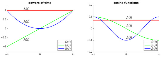
Figure 1. The first three basis functions before normalization in the range $j\in [-k,k]$: on the left, powers of time; on the right, cosine functions.

The LBF estimator has the form [14]

$$\begin{array}{cc}\hfill & {\widehat{\mathit{\theta }}}^{\mathrm{LBF}}\left(t\right)={\mathbf{F}}_0{\widehat{\mathbf{\alpha }}}^{\mathrm{LBF}}\left(t\right)\hfill \end{array}$$

(6)

$$\begin{array}{cc}\hfill & {\widehat{\mathbf{\alpha }}}^{\mathrm{LBF}}\left(t\right)=\underset{\mathbf{\alpha }}{argmin}\mathbf{\sum }_{j=-k}^k{|y(t+j)-{\mathbf{\alpha }}^{\mathrm{H}}\mathit{\psi }(t,j)|}^2\hfill \\ \hfill & ={\left[\mathbf{\sum }_{j=-k}^k\mathit{\psi }(t,j)\mathit{\psi }{(t,j)}^{\mathrm{H}}\right]}^{-1}\left[\mathbf{\sum }_{j=-k}^k\mathit{\psi }(t,j)y^{*}(t+j)\right]\hfill \end{array}$$

(7)

where ${\mathbf{F}}_0=\mathbf{F}\left(0\right)={\mathbf{I}}_n\otimes {\mathbf{f}}_0^{\mathrm{H}},{\mathbf{f}}_0=\mathbf{f}\left(0\right)$.

An essential property of LBF is that it performs non-causal identification, reducing estimation delay but introducing decision delay. The number of estimated hyperparameters $nm$ determines the minimum window length K, which must be substantially greater than $nm$ to prevent numerical issues. Unfortunately, the LBF technique requires inverting an $nm\times nm$ matrix at every instant t, posing a significant computational drawback.

To help readers understand the concept of the LBF approach, it is illustrated here using results obtained for a non-stationary one-tap FIR system described by

$$\begin{array}{c}\hfill y\left(t\right)={\theta }_1\left(t\right)u\left(t\right)+e\left(t\right),\end{array}$$

(8)

where the input $u\left(t\right)$ is a zero-mean, unit-variance, white binary sequence ($\pm 1$). The coefficient ${\theta }_1\left(t\right)$ is modeled as a sinusoidal linear chirp, and the variance of the measurement white Gaussian noise $e\left(t\right)$ is set to ensure an average signal-to-noise ratio of $\mathrm{SNR}=30\mathrm{dB}$. Unlike classical parameter estimation methods, the LBF approach does not require restrictive assumptions such as local stationarity or slow parameter variations. Instead, the local evolution of the parameter is directly represented as a linear combination of basis functions. Figure 2, Figure 3 and Figure 4 demonstrate the estimation capabilities of the LBF approach and emphasize the importance of proper selection of the design parameters k and m.

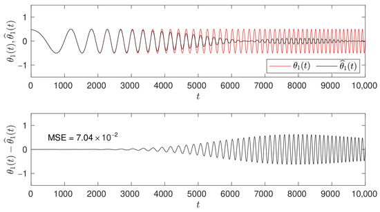
Figure 2. From top to bottom: the true parameter trajectory (red) with the LBF parameter estimate superimposed (black) for $k=200$ and $m=5$; and, at the bottom, the corresponding estimation error along with the mean square estimation error (MSE).

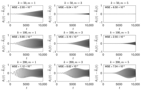
Figure 3. This figure shows $3\times 3$ grid of plots of the estimation error ${\theta }_1\left(t\right)-{\widehat{\theta }}_1\left(t\right)$ for different LBF settings, obtained for all combinations of $k\in [50,100,200]$ and $m\in [1,3,5]$. In each plot, the parameter mean square estimation error (MSE) is displayed in the top-left corner.

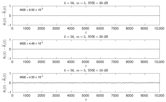
Figure 4. The parameter estimation error ${\theta }_1\left(t\right)-{\widehat{\theta }}_1\left(t\right)$ for different SNR levels $[10,20,30]$ dB for the setting $k=50$ and $m=5$. In each plot, the parameter mean square estimation error (MSE) is shown in the top-left corner.

Figure 2 presents, from top to bottom, the true parameter trajectory (red) with the LBF parameter estimate superimposed (black) for $k=200$ and $m=5$, followed by the estimation error, ${\theta }_1\left(t\right)-{\widehat{\theta }}_1\left(t\right)$. The LBF estimation was initialized before $t=0$ and continued beyond $t=$ 10,000. The chosen values of $k=200$ and $m=5$ yield a small parameter estimation error as long as the parameter variations are moderate. However, when the parameter begins to vary faster, a better choice of k and m is necessary to maintain satisfactory tracking performance.

Figure 3 presents a $3\times 3$ grid of plots showing the estimation error ${\theta }_1\left(t\right)-{\widehat{\theta }}_1\left(t\right)$ for different LBF settings, obtained for all combinations of $k\in [50,100,200]$ and $m\in [1,3,5]$. The selection of these design parameters depends on the rate at which the system parameters vary. For constant parameters, one would typically choose a relatively large window size K and set $m=1$. Note that for $m=1$, the basis function approach reduces to the classical least squares method. For slowly time-varying parameters, a smaller value of k and a larger number of basis functions m becomes beneficial. In the case of faster changing parameters, m should be increased further, and an appropriate window size K must be selected to achieve a favorable mean squared estimation error, shown in the top left corner of each plot. The improvement over the classical least squares method (case $m=1$) is substantial when additional basis functions are used (case $m>1$)—compare, for example, the plots for $k=50,m=1$, and $k=50,m=5$.

Figure 4 presents how different SNR levels $[10,20,30]$ dB impact the parameter estimation error. In this simulated experiment, for $k=50$ and $m=5$, the MSE increased by approximately a factor of 10 each time the SNR dropped by 10 dB.

2.2. fLBF Estimators

As shown in [29,30], under assumptions ($\mathcal{A}$1)–($\mathcal{A}$3), the LBF estimates ${\widehat{\mathbf{\alpha }}}^{\mathrm{LBF}}\left(t\right)$ and ${\widehat{\mathit{\theta }}}^{\mathrm{LBF}}\left(t\right)$ can be approximated by the following computationally fast formulas:

$$\begin{array}{cc}\hfill {\widehat{\mathbf{\alpha }}}^{\mathrm{fLBF}}\left(t\right)& =\underset{\mathbf{\alpha }}{argmin}\mathbf{\sum }_{j=-k}^k\left|\right|\tilde{\mathit{\theta }}(t+j)-\mathbf{F}\left(j\right)\mathbf{\alpha }{\left|\right|}_2^2\hfill \end{array}$$

(9)

$$\begin{array}{cc}\hfill {\widehat{\mathit{\theta }}}^{\mathrm{fLBF}}\left(t\right)& ={\mathbf{F}}_0{\widehat{\mathbf{\alpha }}}^{\mathrm{fLBF}}\left(t\right)=\mathbf{\sum }_{j=-k}^{k}h\left(j\right)\tilde{\mathit{\theta }}(t+j)\hfill \end{array}$$

(10)

where

$$\begin{array}{c}\hfill h\left(j\right)={\mathbf{f}}_0^{\mathrm{H}}\mathbf{f}\left(j\right),j\in I_k\end{array}$$

(11)

denotes the impulse response of the FIR filter associated with the LBF estimator, and $\left\{\tilde{\mathit{\theta }}\left(t\right)\right\}$ denotes the vector of pre-estimated trajectories. These pre-estimates can be obtained through “inverse filtering” of the estimates yielded by the exponentially weighted least squares (EWLS) algorithm

$$\begin{array}{c}\hfill {\widehat{\mathit{\theta }}}^{\mathrm{EWLS}}\left(t\right)=\underset{\mathit{\theta }}{argmin}\mathbf{\sum }_{j=0}^{t-1}{\lambda }^j{|y(t-j)-{\mathit{\theta }}^{\mathrm{H}}\mathit{\phi }(t-j)|}^2\end{array}$$

(12)

where $\lambda ,0<\lambda <1$, denotes the forgetting constant. The short-memory EWLS estimates can be computed using the well-known recursive algorithm [4]:

$$\begin{array}{cc}\hfill \epsilon \left(t\right)& =y\left(t\right)-{\left[{\widehat{\mathit{\theta }}}^{\mathrm{EWLS}}(t-1)\right]}^{\mathrm{H}}\mathit{\phi }\left(t\right)\hfill \end{array}$$

(13)

$$\begin{array}{cc}\hfill \mathbf{k}\left(t\right)& ={\displaystyle \frac{\mathbf{R}(t-1)\mathit{\phi }\left(t\right)}{\lambda +{\mathit{\phi }}^{\mathrm{H}}\left(t\right)\mathbf{R}(t-1)\mathit{\phi }\left(t\right)}}\hfill \end{array}$$

(14)

$$\begin{array}{cc}\hfill {\widehat{\mathit{\theta }}}^{\mathrm{EWLS}}\left(t\right)& ={\widehat{\mathit{\theta }}}^{\mathrm{EWLS}}(t-1)+\mathbf{k}\left(t\right){\epsilon }^{\ast }\left(t\right)\hfill \end{array}$$

(15)

$$\begin{array}{cc}\hfill \mathbf{R}\left(t\right)& ={\displaystyle \frac{1}{\lambda }}[{\mathbf{I}}_n-\mathbf{k}\left(t\right){\mathit{\phi }}^{\mathrm{H}}\left(t\right)]\mathbf{R}(t-1)\hfill \end{array}$$

(16)

with initial conditions ${\widehat{\mathit{\theta }}}^{\mathrm{EWLS}}\left(0\right)=0$ and $\mathbf{R}\left(0\right)=c{\mathbf{I}}_n$, where c denotes a large positive constant. Alternatively, to reduce the computational cost, one can use the iterative dichotomous coordinate descent (DCD) algorithm described in [31].

The inverse filtering formula has the form

$$\begin{array}{c}\hfill \tilde{\mathit{\theta }}\left(t\right)=L_t{\widehat{\mathit{\theta }}}^{\mathrm{EWLS}}\left(t\right)-\lambda L_{t-1}{\widehat{\mathit{\theta }}}^{\mathrm{EWLS}}(t-1)\end{array}$$

(17)

where $L_t={\mathbf{\sum }}_{j=0}^{t-1}{\lambda }^j=\lambda L_{t-1}+1,L_0=1$, denotes the effective width of the exponential window. For large values of t, when the effective window width reaches its steady state value $L_{\infty }=1/(1-\lambda )$, the Formula (17) can be replaced with

$$\begin{array}{c}\hfill \tilde{\mathit{\theta }}\left(t\right)={\displaystyle \frac{1}{1-\lambda }}\left[{\widehat{\mathit{\theta }}}^{\mathrm{EWLS}}\left(t\right)-\lambda {\widehat{\mathit{\theta }}}^{\mathrm{EWLS}}(t-1)\right].\end{array}$$

(18)

The recommended choice of the forgetting factor [29], which performs well in practice, is

$$\begin{array}{c}\hfill \lambda =max\{0.9,1-2/n\}.\end{array}$$

(19)

For $\lambda =1-2/n$, the effective window length $L_{\infty }$ is approximately equal to half the number of estimated coefficients, i.e., $n/2$. As $L_{\infty }$ increases, the mean square deviation of ${\widehat{\mathit{\theta }}}^{\mathrm{EWLS}}\left(t\right)$ from $\mathit{\theta }\left(t\right)$ becomes increasingly dominated by the bias error, which arises primarily because the estimated parameter trajectory lags behind the true trajectory. Therefore, to achieve a favorable bias–variance trade-off, $L_{\infty }$ should remain relatively small.

According to [29], under assumptions ($\mathcal{A}$1)–($\mathcal{A}$3), the pre-estimate $\tilde{\mathit{\theta }}\left(t\right)$ is approximately unbiased, i.e., as follows:

$$\begin{array}{c}\hfill \tilde{\mathit{\theta }}\left(t\right)\approxeq \mathit{\theta }\left(t\right)+\mathbf{z}\left(t\right),\end{array}$$

(20)

where $\mathbf{z}\left(t\right)$ denotes approximately zero-mean white noise with large covariance matrix $\mathrm{cov}\left[\mathbf{z}\left(t\right)\right]={\sigma }_z^2{\mathbf{I}}_n$. The unbiasedness property comes at the cost of significant variability. The fLBF estimate ${\widehat{\mathit{\theta }}}^{\mathrm{fLBF}}\left(t\right)$ can thus be interpreted as a denoised version of $\tilde{\mathit{\theta }}\left(t\right)$ obtained via the basis function approach.

The fLBF approach is illustrated using the same one-tap FIR example as the LBF method—see (8). Figure 5 presents the pre-estimates (A, black) obtained by inverse filtering of the EWLS estimates using Formula (18), with $\lambda =0.9$ at an SNR level of 10 dB. These pre-estimates were then denoised using the FIR filter impulse response defined in (11) for $k=50$ and $m=5$, resulting in the final fLBF estimates shown in (B, black). In this simple case, the estimation error for the fLBF results shown in (C) closely matches that of the LBF approach.

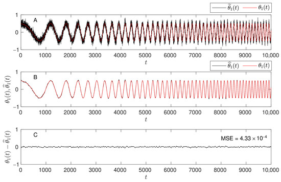
Figure 5. From top to bottom: (A) the true parameter trajectory (red) with pre-estimates superimposed (black) at an SNR level of 10 dB; (B) the true parameter trajectory (red) with fLBF estimates superimposed (black) for $k=50$ and $m=5$; (C) the estimation error, ${\theta }_1\left(t\right)-{\widehat{\theta }}_1\left(t\right)$, with the mean square estimation error (MSE) indicated in the top-right corner.

2.3. Regularized fLBF Estimators

Denote by ${\left|\right|\mathbf{x}\left|\right|}_2=\sqrt{{\mathbf{\sum }}_{i=1}^n{\left|x_i\right|}^2}$ the ${\mathit{\ell }}^2$ norm of a complex-valued vector $\mathbf{x}={[x_1,\dots ,x_n]}^{\mathrm{T}}$, and by ${\left|\right|\mathbf{x}\left|\right|}_1={\mathbf{\sum }}_{i=1}^n\left|x_i\right|$ its ${\mathit{\ell }}^1$ norm. Finally, let ${\left|\right|\mathbf{x}\left|\right|}_{\mathbf{A}}=\sqrt{{\mathbf{x}}^{\mathrm{H}}\mathbf{A}\mathbf{x}}$, where $\mathbf{A}$ denotes a $n\times n$ positive definite Hermitian matrix.

The LASSO-type regularized fLBF estimator, defined as

$$\begin{array}{cc}\hfill {\widehat{\mathbf{\alpha }}}^{\mathrm{LASSO}}\left(t\right)& =\underset{\mathbf{\alpha }}{argmin}\left\{\mathbf{\sum }_{j=-k}^k\left|\right|\tilde{\mathit{\theta }}(t+j)-{\mathbf{F}\left(j\right)\mathbf{\alpha }\left|\right|}_2^2+{\eta \left|\right|\mathbf{\alpha }\left|\right|}_1+\mu \left|\right|{\mathbf{F}}_0\mathbf{\alpha }{\left|\right|}_1\right\}\hfill \end{array}$$

(21)

$$\begin{array}{cc}\hfill {\widehat{\mathit{\theta }}}^{\mathrm{LASSO}}\left(t\right)& ={\mathbf{F}}_0{\widehat{\mathbf{\alpha }}}^{\mathrm{LASSO}}\left(t\right)\hfill \end{array}$$

(22)

where $\eta ,\mu >0$ denote regularization constants, which incorporates two regularizers. When both regularization constants are set to zero, the solution reduces to the standard fLBF approach. These constants allow for fine-tuning the degree of shrinkage applied to the estimates as they approach zero. Setting higher regularization constants increases shrinkage but does not eliminate parameters entirely, unlike LASSO, which can set coefficients to zero. The first regularizer, ${\eta \left|\right|\mathbf{\alpha }\left(t\right)\left|\right|}_1$, promotes sparseness in the frequency domain by penalizing the excessive number of basis functions used to approximate the time evolution of channel parameters ${\theta }_1\left(t\right),\dots ,{\theta }_n\left(t\right)$. The second regularizer, $\mu \left|\right|{\mathbf{F}}_0{\mathbf{\alpha }\left|\right|}_1={\mu \left|\right|\mathit{\theta }\left(t\right)\left|\right|}_1$, promotes sparseness in the time/lag domain by penalizing non-zero components of the vector $\mathit{\theta }\left(t\right)$. With the inclusion of the second regularizer, schemes (21) and (22) serve as a group LASSO solution, enhancing model sparsity at both individual (hyperparameter) and group (parameter) component levels [32].

Due to the lack of a closed-form solution to the minimization problem in (21) and (22), numerical search is necessary, posing a drawback for sliding window estimation. Similarly, selecting optimal regularization gains $\eta$ and $\mu$ presents a similar challenge. To mitigate these issues, we propose replacing the ${\mathit{\ell }}^1$ regularization terms in (21) with appropriately reweighted ${\mathit{\ell }}^2$ regularizers. Reweighting is a known optimization technique [33,34]. Note that the ${\mathit{\ell }}^1$ norm of the vector $\mathbf{x}$ can be expressed as

$$\begin{array}{c}\hfill {\left|\right|\mathbf{x}\left|\right|}_1=\mathbf{\sum }_{i=1}^n{\displaystyle \frac{x_i^{\ast }{x}_i}{|x_i|}}={\mathbf{x}}^{\mathrm{H}}\mathrm{W}\mathbf{x}={\left|\right|\mathbf{x}\left|\right|}_{\mathrm{W}}^2\end{array}$$

(23)

where $\mathbf{W}=\mathrm{diag}\left\{\right|x_1{|}^{-1},\dots ,\left|x_n{|}^{-1}\right\}$ is the weight matrix. In order to apply the reweighting technique directly to the vector $\mathbf{\alpha }\left(t\right)$

$$\begin{array}{c}\hfill {\left|\right|\mathbf{\alpha }\left(t\right)\left|\right|}_1=\mathbf{\sum }_{i=1}^n\mathbf{\sum }_{l=1}^m{\displaystyle \frac{a_{il}^{\ast }\left(t\right)a_{il}\left(t\right)}{|a_{il}\left(t\right)|}}={\mathbf{\alpha }}^{\mathrm{H}}\left(t\right)\mathbf{W}\mathbf{\alpha }\left(t\right)={\left|\right|\mathbf{\alpha }\left(t\right)\left|\right|}_{\mathbf{W}}^2\end{array}$$

(24)

one would need to know the true trajectories of the system hyperparameters $a_{il}\left(t\right)$, which are assumed to be unknown. Therefore, the weight matrix $\mathbf{W}$ is initialized based on the estimated values ${\widehat{a}}_{il}^{\mathrm{fLBF}}\left(t\right)$ obtained from the fLBF algorithm. Using the reweighting technique together with the fLBF approach, one arrives at the approximations

$$\begin{array}{cc}\hfill {\left|\right|\mathbf{\alpha }\left(t\right)\left|\right|}_1& {\cong \left|\right|\mathbf{\alpha }\left(t\right)\left|\right|}_{\mathbf{\Delta }\left(t\right)}^2\hfill \end{array}$$

(25)

$$\begin{array}{cc}\hfill \mathbf{\Delta }\left(t\right)& =\mathrm{bl}\mathrm{diag}\{{\mathbf{\Delta }}_1\left(t\right),\dots ,{\mathbf{\Delta }}_n\left(t\right)\}\hfill \end{array}$$

(26)

$$\begin{array}{cc}\hfill {\mathbf{\Delta }}_i\left(t\right)& =\mathrm{diag}\{{\delta }_{i1}\left(t\right),\dots ,{\delta }_{im}\left(t\right)\}\hfill \end{array}$$

(27)

$$\begin{array}{cc}\hfill {\delta }_{il}\left(t\right)& =|{\widehat{a}}_{il}^{\mathrm{fLBF}}{\left(t\right)|}^{-1},i=1,\dots ,n,l=1,\dots ,m\hfill \end{array}$$

(28)

and

$$\begin{array}{cc}\hfill {\left|\right|\mathit{\theta }\left(t\right)\left|\right|}_1& =\left|\right|{\mathbf{F}}_0{\mathbf{\alpha }\left(t\right)\left|\right|}_1{\cong \left|\right|\mathbf{\alpha }\left(t\right)\left|\right|}_{{\mathbf{F}}_0^{\mathrm{H}}\mathbf{\Gamma }\left(t\right){\mathbf{F}}_0}^2\hfill \end{array}$$

(29)

$$\begin{array}{cc}\hfill \mathbf{\Gamma }\left(t\right)& =\mathrm{diag}\{{\gamma }_1\left(t\right),\dots ,{\gamma }_n\left(t\right)\}\hfill \end{array}$$

(30)

$$\begin{array}{cc}\hfill {\gamma }_i\left(t\right)& =|{\widehat{\theta }}^{\mathrm{fLBF}}{\left(t\right)|}^{-1},i=1,\dots ,n.\hfill \end{array}$$

(31)

This leads to the following approximate version of (21) and (22), further referred to as the fast regularized LBF (fRLBF) estimator

$$\begin{array}{cc}\hfill {\widehat{\mathbf{\alpha }}}^{\mathrm{fRLBF}}\left(t\right)& =\underset{\mathbf{\alpha }}{argmin}\left\{\mathbf{\sum }_{j=-k}^k\left|\right|\tilde{\mathit{\theta }}(t+j)-{\mathbf{F}\left(j\right)\mathbf{\alpha }\left|\right|}_2^2+{\left|\right|\mathbf{\alpha }\left|\right|}_{\mathbf{\Sigma }(t;\eta ,\mu )}^2\right\}\hfill \\ \hfill & ={[{\mathbf{I}}_{nm}+\mathbf{\Sigma }(t;\eta ,\mu )]}^{-1}{\widehat{\mathbf{\alpha }}}^{\mathrm{fLBF}}\left(t\right)\hfill \end{array}$$

(32)

$$\begin{array}{cc}\hfill {\widehat{\mathit{\theta }}}^{\mathrm{fRLBF}}\left(t\right)& ={\mathbf{F}}_0{\widehat{\mathbf{\alpha }}}^{\mathrm{fRLBF}}\left(t\right)\hfill \end{array}$$

(33)

where

$$\begin{array}{c}\hfill \begin{array}{cc}\hfill \mathbf{\Sigma }(t;\eta ,\mu )& =\eta \mathbf{\Delta }\left(t\right)+\mu {\mathbf{F}}_0^{\mathrm{H}}\mathbf{\Gamma }\left(t\right){\mathbf{F}}_0\hfill \\ \hfill & =\eta \mathbf{\Delta }\left(t\right)+\mu \Gamma \left(t\right)\otimes \left({\mathbf{f}}_0{\mathbf{f}}_0^{\mathrm{H}}\right).\hfill \end{array}\end{array}$$

(34)

The last transition in (34) follows from the identity

$$\begin{array}{c}\hfill (\mathbf{A}\otimes \mathbf{B})(\mathbf{C}\otimes \mathbf{D})=\left(\mathbf{A}\mathbf{C}\right)\otimes \left(\mathbf{B}\mathbf{D}\right)\end{array}$$

(35)

which holds true for Kronecker products, provided that all dimensions match.

Utilizing the fact that the matrix $\mathbf{\Sigma }(t;\eta ,\mu )$ is block diagonal

$$\begin{array}{cc}\hfill \mathbf{\Sigma }(t;\eta ,\mu )& =\mathrm{bl}\mathrm{diag}\{{\mathbf{\Sigma }}_1(t;\eta ,\mu ),\dots ,{\mathbf{\Sigma }}_n(t;\eta ,\mu )\}\hfill \end{array}$$

(36)

$$\begin{array}{cc}\hfill {\mathbf{\Sigma }}_i(t;\eta ,\mu )& =\eta {\mathbf{\Delta }}_i\left(t\right)+\mu {\gamma }_i\left(t\right){\mathbf{f}}_0{\mathbf{f}}_0^{\mathrm{H}},i=1,\dots ,n\hfill \end{array}$$

(37)

the relationship (32) and (33) can be rewritten in a simpler, decomposed form

$$\begin{array}{cc}\hfill {\widehat{\mathbf{\alpha }}}_i^{\mathrm{fRLBF}}\left(t\right)& ={[{\mathbf{I}}_m+{\mathbf{\Sigma }}_i(t;\eta ,\mu )]}^{-1}{\widehat{\mathbf{\alpha }}}_i^{\mathrm{fLBF}}\left(t\right)\hfill \end{array}$$

(38)

$$\begin{array}{cc}\hfill {\widehat{\theta }}_i^{\mathrm{fRLBF}}\left(t\right)& ={\mathbf{f}}_0^{\mathrm{H}}{\widehat{\mathbf{\alpha }}}_i^{\mathrm{fRLBF}}\left(t\right)\hfill \\ \hfill i& =1,\dots ,n\hfill \end{array}$$

(39)

where

$$\begin{array}{c}\hfill {\widehat{\mathbf{\alpha }}}_i^{\mathrm{fLBF}}\left(t\right)=\mathbf{\sum }_{j=-k}^k{\tilde{\mathit{\theta }}}_i(t+j)\mathbf{f}\left(j\right).\end{array}$$

(40)

LASSO estimators discard insignificant components by shrinking them to zero. The proposed fRLBF scheme approximates this behavior. When the estimates ${\widehat{a}}_{il}^{\mathrm{fLBF}}\left(t\right)$ and ${\widehat{\theta }}_i^{\mathrm{fLBF}}\left(t\right)$ are very small in magnitude, the weights ${\delta }_{il}\left(t\right)$ and ${\gamma }_i\left(t\right)$ in (38) and (39) become very large, effectively shrinking the corresponding fLBF estimates towards zero.

Remark 1.

Communication channels typically exhibit a decaying power profile due to spreading and absorption loss, which can be modeled by assuming that

$$\begin{array}{c}\hfill \mathrm{var}\left[{\theta }_i\left(t\right)\right]\propto {\xi }^{i-1},i=1,\dots ,n\end{array}$$

where $\xi ,0<\xi <1$, represents the decay rate of the exponential power envelope. Incorporating this prior knowledge into the estimation scheme is straightforward by setting

$$\begin{array}{c}\hfill {\gamma }_i\left(t\right)=[{\xi }^{{\displaystyle \frac{i-1}{2}}}|{\widehat{\theta }}_i^{\mathrm{fLBF}}\left(t\right){\left|\right]}^{-1}\end{array}$$

(41)

This corresponds to replacing the second regularizer in (21) with the weighted ${\mathit{\ell }}^1$ norm $\mathit{\theta }\left(t\right)$ given by

$$\begin{array}{c}\hfill \mathbf{\sum }_{i=1}^n{\displaystyle \frac{|{\theta }_i|}{{\xi }^{\frac{i-1}{2}}}}\end{array}$$

Hence, adjusting ξ according to the decaying power profile leads to improved estimation results.

2.4. Computational Complexity of fRLBF Estimators

First of all, we note that for the selected basis set, powers of time, the fLBF estimates are recursively computable [14]. This is a direct consequence of the recursive computability of $\mathbf{f}\left(j\right)$. It is easy to check that

$$\begin{array}{c}\hfill \mathbf{f}\left(j\right)={\mathbf{\Lambda }}_{m|k}\mathbf{f}(j+1)\end{array}$$

(42)

where

$$\begin{array}{c}\hfill {\mathbf{\Lambda }}_{m|k}=\left[\begin{array}{cccc}1& 0& \dots & 0\\ -\frac{1}{k}& 1& 0& \\ & \ddots & \ddots & \\ {\displaystyle \frac{\left(\genfrac{}{}{0pt}{}{m-1}{m-1}\right)}{{(-k)}^{m-1}}}& {\displaystyle \frac{\left(\genfrac{}{}{0pt}{}{m-1}{m-2}\right)}{{(-k)}^{m-2}}}& \dots & 1\end{array}\right]\end{array}$$

(43)

denotes the $m\times m$ transition matrix, and $\left({\displaystyle \genfrac{}{}{0pt}{}{n}{k}}\right)={\displaystyle \frac{n!}{k!(n-k)!}}$ denotes binomial coefficient, leading to the following recursive formula:

$$\begin{array}{c}\hfill {\widehat{\mathbf{\alpha }}}_i^{\mathrm{fLBF}}(t+1)={\mathbf{\Lambda }}_{m|k}[{\widehat{\mathbf{\alpha }}}_i^{\mathrm{fLBF}}\left(t\right)-{\tilde{\theta }}_i(t-k)\mathbf{f}(-k)]+{\tilde{\theta }}_i(t+k+1)\mathbf{f}\left(k\right).\end{array}$$

(44)

All n fLBF estimates can be obtained at the cost of $(m^2+2m)n$ complex flops (complex multiply-add operations) per time updated. Importantly, this cost remains independent of the analysis window width K.

To estimate the computational burden of the second estimation stage, consider the matrix inversion lemma [4]

$$\begin{array}{c}\hfill \begin{array}{c}\hfill {[{\mathbf{I}}_m+{\mathbf{\Sigma }}_i(t;\eta ,\mu )]}^{-1}={[{\mathbf{G}}_i(t;\eta )+\mu {\gamma }_i\left(t\right){\mathbf{f}}_0{\mathbf{f}}_0^{\mathrm{H}}]}^{-1}\\ \hfill ={\mathbf{G}}_i^{-1}(t;\eta )-\mu {\gamma }_i\left(t\right){\displaystyle \frac{{\mathbf{G}}_i^{-1}(t;\eta ){\mathbf{f}}_0{\mathbf{f}}_0^{\mathrm{H}}{\mathbf{G}}_i^{-1}(t;\eta )}{1+\mu {\gamma }_i\left(t\right){\mathbf{f}}_0^{\mathrm{H}}{\mathbf{G}}_i^{-1}(t;\eta ){\mathbf{f}}_0}}\end{array}\end{array}$$

(45)

where

$$\begin{array}{cc}\hfill {\mathbf{G}}_i^{-1}(t;\eta )& =\mathrm{diag}\{g_{i1}(t;\eta ),\dots ,g_{im}(t;\eta )\}\hfill \end{array}$$

(46)

$$\begin{array}{cc}\hfill g_{il}(t;\eta )& ={[1+\eta {\delta }_{il}\left(t\right)]}^{-1}.\hfill \end{array}$$

(47)

Exploiting the diagonal nature of the matrix ${\mathbf{G}}_i^{-1}(t;\eta )={[{\mathbf{I}}_m+\eta {\mathbf{\Delta }}_i\left(t\right)]}^{-1}$ and the fact that ${\mathbf{f}}_0={[1,\dots ,1]}^{\mathrm{T}}$, the cost of updating the estimates ${\widehat{\mathbf{\alpha }}}_i^{\mathrm{fRLBF}}\left(t\right),i=1,\dots ,n$, is approximately $4mn$ complex flops, after neglecting terms of order $O\left(n\right)$ and $O\left(m\right)$. Additional $mn$ complex additions are required to update ${\widehat{\theta }}_i^{\mathrm{fRLBF}}\left(t\right),i=1,\dots ,n$.

Finally, computation of $g_{il}(t;\eta ),i=1,\dots ,n,l=1,\dots ,m$, requires $mn$ complex flops, $mn$ square root operations, and $mn$ real divisions. Hence, the cost of running the two-stage procedure is roughly $(m^2+6m)n$ complex flops, $mn$ complex additions, $mn$ square root operations, and $mn$ real divisions per time update.

Remark 2.

Since all eigenvalues of the matrix ${\mathbf{\Lambda }}_{m|k}$ are located on the unit circle in the complex plane, the recursive algorithm (44) is not exponentially stable but only marginally stable. This means that it has the tendency to diverge at a slow (linear) rate when the number of time steps becomes very large. To prevent numerical problems caused by the unbounded accumulation of round-off errors, the algorithm (44) should be periodically reset by directly computing ${\widehat{\mathbf{\alpha }}}_i^{\mathrm{fLBF}}\left(t\right)$ using (40). In the absence of an automated mechanism for detecting numerical issues and initiating timely resets, a practical strategy was employed. To balance the computational efficiency of the recursive formulation with numerical stability, algorithm (44) was reset every 1000 steps, with the fLBF estimates re-initialized directly from the local estimation window at these intervals [35].

2.5. Multi-Step Procedure of fRLBF Estimators

The fRLBF scheme described above is a two-step procedure. For improved performance, one can consider a multi-step procedure, similar to those described in [33,34], at the expense of increased computational complexity, as follows:

$$\begin{array}{cc}\hfill {\widehat{\mathbf{\alpha }}}_i^{\mathrm{fRLBF}}(t,j+1)& ={[{\mathbf{I}}_m+{\mathbf{\Sigma }}_i(t,j;\eta ,\mu )]}^{-1}{\widehat{\mathbf{\alpha }}}_i^{\mathrm{fLBF}}\left(t\right)\hfill \end{array}$$

(48)

$$\begin{array}{cc}\hfill {\widehat{\mathit{\theta }}}_i^{\mathrm{fRLBF}}(t,j+1)& ={\mathbf{f}}_0^{\mathrm{H}}{\widehat{\mathbf{\alpha }}}_i^{\mathrm{fRLBF}}(t,j+1)\hfill \\ \hfill i=1,\dots ,n,& j=1,2,\dots \hfill \end{array}$$

(49)

where

$$\begin{array}{cc}\hfill {\mathbf{\Sigma }}_i(t,j;\eta ,\mu )& =\eta {\mathbf{\Delta }}_i(t,j)+\mu {\gamma }_i(t,j){\mathbf{f}}_0{\mathbf{f}}_0^{\mathrm{H}}\hfill \end{array}$$

(50)

$$\begin{array}{cc}\hfill {\mathbf{\Delta }}_i(t,j)& =\mathrm{diag}\{{\delta }_{i1}(t,j),\dots ,{\delta }_{im}(t,j)\}\hfill \end{array}$$

(51)

$$\begin{array}{cc}\hfill {\delta }_{il}(t,j)& =|{\widehat{a}}_{il}^{\mathrm{fRLBF}}{(t,j)|}^{-1}\hfill \end{array}$$

(52)

$$\begin{array}{cc}\hfill {\gamma }_i(t,j)& =|{\widehat{\theta }}_i^{\mathrm{fRLBF}}{(t,j)|}^{-1}\hfill \\ \hfill i=1,\dots ,& n,l=1,\dots ,m\hfill \end{array}$$

(53)

and ${\widehat{\mathbf{\alpha }}}_i^{\mathrm{fRLBF}}(t,1)={\widehat{\mathbf{\alpha }}}_i^{\mathrm{fLBF}}\left(t\right)$, ${\widehat{\theta }}_i^{\mathrm{fRLBF}}(t,1)={\widehat{\theta }}_i^{\mathrm{fLBF}}\left(t\right)$. To avoid numerical issues, the magnitudes of $|{\widehat{a}}_{il}^{\mathrm{fRLBF}}(t,j)|$ and $|{\widehat{\theta }}_i^{\mathrm{fRLBF}}(t,j)|$ should be replaced by a fixed number before inversion if they are too close to zero. This iterative procedure can be implemented efficiently without requiring inversion of an $m\times m$ matrix, as demonstrated in the previous section (see (45)–(47)).

It is important to emphasize that the proposed fRLBF approach is not iterative in the same sense as algorithms like ISTA, where a stopping criterion is required to prevent excessive computational cost once convergence is achieved, or OMP, where limiting the number of selected atoms is essential not only to control computational cost but also to avoid increased estimation error due to over-parameterization. In the fRLBF approach, estimation convergence is determined by how the pre-estimates are obtained and by the careful selection of fLBF hyperparameters. The multi-step procedure is intended solely for fine-tuning the results, with each iteration involving $6mn$ complex flops, $mn$ square root operations, and $mn$ real divisions. While increasing the number of iterations can yield incremental improvements in estimation accuracy, typical criteria—such as absolute or relative changes in parameter values—require selecting an appropriate convergence threshold. If not properly chosen, this can lead to unnecessary iterations and reduced computational efficiency. In the case of the time-varying FIR model, the optimal number of iterations is application-dependent and should be selected to balance estimation accuracy with computational efficiency. Based on empirical observations, the best trade-off was achieved by stopping the procedure after the second iteration.

2.6. Selection of Regularization Gains

The choice of regularization gains is an important part of regularized estimation—if the values of $\eta$ and $\mu$ are not chosen appropriately, the accuracy of fRLBF estimates can be worse than the accuracy of their not regularized versions. In this section, we will present three approaches to solve this problem.

2.6.1. Empirical Bayes Approach

Bayesian redefinition of the optimization problem (32) and (33) is based on the observation that minimization of the quadratic cost function

$$\begin{array}{c}\hfill \mathbf{\sum }_{j=-k}^k\left|\right|\tilde{\mathit{\theta }}(t+j)-{\mathbf{F}\left(j\right)\mathbf{\alpha }\left|\right|}_2^2+{\left|\right|\mathbf{\alpha }\left|\right|}_{\mathbf{\Sigma }}^2\end{array}$$

is equivalent to the maximization of the expression

$$\begin{array}{c}\hfill exp\left\{-{\displaystyle \frac{1}{2{\sigma }_z^2}}\mathbf{\sum }_{j=-k}^k\left|\right|\tilde{\mathit{\theta }}(t+j)-\mathbf{F}\left(j\right)\mathbf{\alpha }{\left|\right|}_2^2\right\}\times exp\left\{-{\displaystyle \frac{1}{{\sigma }_z^2}}{\left|\right|\mathbf{\alpha }\left|\right|}_{\mathbf{\Sigma }}^2\right\}\end{array}$$

(54)

which can be given a probabilistic interpretation. Assuming that the pre-estimation noise $\mathbf{z}\left(t\right)$ is Gaussian, the first term in (54) represents the conditional data distribution (likelihood)

$$\begin{array}{cc}\hfill & p(\Theta \left(t\right)|\mathbf{\alpha },{\sigma }_z^2)={\displaystyle \frac{1}{{\left(2\pi {\sigma }_z^2\right)}^{\frac{M}{2}}}}exp\{-{\displaystyle \frac{1}{2{\sigma }_z^2}}{\left|\right|\mathbf{\alpha }\left|\right|}_2^2\hfill \\ \hfill & +{\displaystyle \frac{1}{2{\sigma }_z^2}}{\mathbf{\alpha }}^{\mathrm{H}}\mathbf{\sum }_{j=-k}^k{\mathbf{F}}^{\mathrm{H}}\left(j\right)\tilde{\mathit{\theta }}(t+j)+{\displaystyle \frac{1}{2{\sigma }_z^2}}\mathbf{\sum }_{j=-k}^k{\tilde{\mathit{\theta }}}^{\mathrm{H}}(t+j)\mathbf{F}\left(j\right)\mathbf{\alpha }\hfill \\ \hfill & -{\displaystyle \frac{1}{2{\sigma }_z^2}}\mathbf{\sum }_{j=-k}^k\left|\right|\tilde{\mathit{\theta }}{(t+j)\left|\right|}_2^2\}\hfill \end{array}$$

(55)

where $\Theta \left(t\right)=\{\tilde{\mathit{\theta }}(t+j),j\in I_k\}$ and $M=Kn$. The second term corresponds to a prior distribution of $\mathbf{\alpha }$

$$\begin{array}{c}\hfill \pi \left(\mathbf{\alpha }\right|\mathbf{\Sigma },{\sigma }_z^2)={\displaystyle \frac{{|\mathbf{\Sigma }|}^{1/2}}{{\left(2\pi {\sigma }_z^2\right)}^{mn/2}}}exp\left\{-{\displaystyle \frac{1}{2{\sigma }_z^2}}{\mathbf{\alpha }}^{\mathrm{H}}\mathbf{\Sigma }\mathbf{\alpha }\right\}\end{array}$$

(56)

where $|\mathbf{\Sigma }|$ denotes the determinant of the matrix $\mathbf{\Sigma }$. The likelihood for the unknown parameters $\mathbf{\Sigma }$ and ${\sigma }_z^2$ can be obtained from (see Appendix A)

$$\begin{array}{c}\hfill L(\mathbf{\Sigma },{\sigma }_z^2)={\int }_{{\mathcal{C}}^{mn}}p(\Theta \left(t\right)|\mathbf{\alpha },{\sigma }_z^2)\pi \left(\mathbf{\alpha }\right|\mathbf{\Sigma },{\sigma }_z^2)d\mathbf{\alpha }\\ \hfill ={\displaystyle \frac{{|\mathbf{\Sigma }|}^{1/2}}{{\left(2\pi {\sigma }_z^2\right)}^{M/2}{|{\mathbf{I}}_{mn}+\mathbf{\Sigma }|}^{1/2}}}exp\left\{-{\displaystyle \frac{\zeta (t;\mu )}{2{\sigma }_z^2}}\right\}\end{array}$$

(57)

where

$$\begin{array}{c}\hfill \zeta (t;\mathbf{\Sigma })=\mathbf{\sum }_{j=-k}^k\left|\right|\tilde{\mathit{\theta }}(t+j){\left|\right|}_2^2-{\left[{\widehat{\mathbf{\alpha }}}^{\mathrm{fLBF}}\left(t\right)\right]}^{\mathrm{H}}{[{\mathbf{I}}_{mn}+\mathbf{\Sigma }]}^{-1}{\widehat{\mathbf{\alpha }}}^{\mathrm{fLBF}}\left(t\right)\end{array}$$

(58)

denotes the residual sum of squares. Good [36] referred to the maximization of (57) as a type II maximum likelihood method, but recently it has been more frequently referred to as the empirical Bayes approach [15,36].

Since the maximum likelihood estimate of the variance ${\sigma }_z^2$ can be obtained in the form ${\widehat{\sigma }}_z^2(\mathbf{\Sigma })=\zeta (t,\mathbf{\Sigma })/M$, the optimal value of the regularization matrix $\mathbf{\Sigma }$ can be obtained by maximizing the concentrated likelihood function $L(\mathbf{\Sigma },{\widehat{\sigma }}_z^2(\mathbf{\Sigma }))$, or equivalently by minimizing the quantity

$$\begin{array}{c}\hfill -2logL(\mathbf{\Sigma },{\sigma }_z^2(\mathbf{\Sigma }))=\mathrm{const}+Mlog{\widehat{\sigma }}_z^2(\mathbf{\Sigma })-log|\mathbf{\Sigma }|+log|{\mathbf{I}}_{mn}+\mathbf{\Sigma }|.\end{array}$$

(59)

In the case of structured matrix of the form $\mathbf{\Sigma }=\mathbf{\Sigma }(t;\eta ,\mu )=\eta \mathbf{\Delta }\left(t\right)+\mu \mathbf{\Gamma }\left(t\right)$, the optimization is restricted to regularization gains $\eta$ and $\mu$. This leads to the following optimization formula (see Appendix B):

$$\begin{array}{c}\hfill \{{\eta }^{\mathrm{opt}},{\mu }^{\mathrm{opt}}\}=arg\underset{\eta ,\mu }{min}J(t;\eta ,\mu )\end{array}$$

(60)

where

$$\begin{array}{c}\hfill \begin{array}{cc}\hfill J(t;\eta ,\mu )& =Mlog\zeta (t;\eta ,\mu )+\mathbf{\sum }_{i=1}^n\mathbf{\sum }_{l=1}^{m}log{\displaystyle \frac{1+\eta {\delta }_{il}\left(t\right)}{\eta {\delta }_{il}\left(t\right)}}\hfill \\ \hfill & +\mathbf{\sum }_{i=1}^{n}log{\displaystyle \frac{1+\mu {\gamma }_i\left(t\right){\mathbf{\sum }}_{l=1}^m\frac{|f_l{\left(0\right)|}^2}{1+\eta {\delta }_{il}\left(t\right)}}{1+\mu {\gamma }_i\left(t\right){\mathbf{\sum }}_{l=1}^m\frac{|f_l{\left(0\right)|}^2}{\eta {\delta }_{il}\left(t\right)}}}.\hfill \end{array}\end{array}$$

(61)

As a practical way of solving the optimization problem, one can consider parallel estimation. In this case, not one but p fRLBF algorithms equipped with different regularization gains $(\eta ,\mu )\in \mathcal{P}=\{({\eta }_1,{\mu }_1),\dots ,({\eta }_p,{\mu }_p)\}$, yielding the estimates ${\widehat{\mathbf{\alpha }}}^{\mathrm{fRLBF}}\left(t\right|\eta ,\mu )$ and ${\widehat{\mathit{\theta }}}^{\mathrm{fRLBF}}\left(t\right|\eta ,\mu )$, are run simultaneously and compared using the empirical Bayes measure of fit (61). At each time instant t, the best fitting values of $\eta$ and $\mu$ are chosen using the grid search

$$\begin{array}{c}\hfill \{\widehat{\eta }\left(t\right),\widehat{\mu }\left(t\right)\}=\underset{(\eta ,\mu )\in \mathcal{P}}{argmin}J(t;\eta ,\mu )\end{array}$$

(62)

and the final estimates for empirical Bayes approach have the form

$$\begin{array}{c}\hfill {\widehat{\mathbf{\alpha }}}^{\mathrm{fRLBF}}\left(t\right|\widehat{\eta }\left(t\right),\widehat{\mu }\left(t\right)),{\widehat{\mathit{\theta }}}^{\mathrm{fRLBF}}\left(t\right|\widehat{\eta }\left(t\right),\widehat{\mu }\left(t\right)).\end{array}$$

(63)

The cost of evaluating (63) is of order $O\left(pmn\right)$ per time update. Note that in this case, the following computational shortcut can be used to evaluate the residual sum of squares:

$$\begin{array}{c}\hfill \begin{array}{cc}\hfill \zeta (t;\eta ,\mu )& =\mathbf{\sum }_{j=-k}^k\left|\right|\tilde{\mathit{\theta }}(t+j){\left|\right|}_2^2-{\left[{\widehat{\mathbf{\alpha }}}^{\mathrm{fLBF}}\left(t\right)\right]}^{\mathrm{H}}{[{\mathbf{I}}_{mn}+\mathbf{\Sigma }(t;\eta ,\mu )]}^{-1}{\widehat{\mathbf{\alpha }}}^{\mathrm{fLBF}}\left(t\right)\hfill \\ \hfill & =\mathbf{\sum }_{i=1}^n\mathbf{\sum }_{j=-k}^k{\left|{\tilde{\theta }}_i(t+j)\right|}^2-\mathbf{\sum }_{i=1}^n{\left[{\widehat{\mathbf{\alpha }}}_i^{\mathrm{fLBF}}\left(t\right)\right]}^{\mathrm{H}}{\widehat{\mathbf{\alpha }}}_i^{\mathrm{fRLBF}}\left(t\right|\eta ,\mu ).\hfill \end{array}\end{array}$$

(64)

Note also that the first term on the right-hand side of (64) can be updated recursively.

2.6.2. Decentralized Approach

Alternatively, following the decomposed form in (38) and (39), we propose to optimize the regularization gains $\eta$ and $\mu$ independently for each ${\widehat{\mathbf{\alpha }}}_i^{\mathrm{fRLBF}}\left(t\right)$, which enhances the flexibility of the approach. Since some of the parameters ${\theta }_i\left(t\right)$ may be static while others time-varying, different regularization gains are necessary. This leads to the decomposed optimization formula

$$\begin{array}{c}\hfill \{{\eta }_i^{\mathrm{opt}},{\mu }_i^{\mathrm{opt}}\}=\underset{{\eta }_i,{\mu }_i}{argmin}{J}_i(t;{\eta }_i,{\mu }_i),i=1,\dots ,n\end{array}$$

(65)

where

$$\begin{array}{c}\hfill \begin{array}{cc}\hfill J_i(t;{\eta }_i,{\mu }_i)& =Klog{\zeta }_i(t;{\eta }_i,{\mu }_i)+\mathbf{\sum }_{l=1}^{m}log{\displaystyle \frac{1+{\eta }_i{\delta }_{il}\left(t\right)}{{\eta }_i{\delta }_{il}\left(t\right)}}\hfill \\ \hfill & +log{\displaystyle \frac{1+{\mu }_i{\gamma }_i\left(t\right){\mathbf{\sum }}_{l=1}^m\frac{|f_l{\left(0\right)|}^2}{1+{\eta }_i{\delta }_{il}\left(t\right)}}{1+{\mu }_i{\gamma }_i\left(t\right){\mathbf{\sum }}_{l=1}^m\frac{|f_l{\left(0\right)|}^2}{{\eta }_i{\delta }_{il}\left(t\right)}}}\hfill \end{array}\end{array}$$

(66)

and

$$\begin{array}{c}\hfill \begin{array}{c}\hfill {\zeta }_i(t;{\eta }_i,{\mu }_i)=\mathbf{\sum }_{j=-k}^k{\left|{\tilde{\theta }}_i(t+j)\right|}^2-{\left[{\widehat{\mathbf{\alpha }}}_i^{\mathrm{fLBF}}\left(t\right)\right]}^{\mathrm{H}}{\widehat{\mathbf{\alpha }}}_i^{\mathrm{fRLBF}}\left(t\right|{\eta }_i,{\mu }_i).\end{array}\end{array}$$

(67)

Similar to the centralized approach, at each time instant t, the best fitting values of ${\eta }_i$ and ${\mu }_i$ are chosen using the grid search

$$\begin{array}{c}\hfill \{{\widehat{\eta }}_i\left(t\right),{\widehat{\mu }}_i\left(t\right)\}=\underset{({\eta }_i,{\mu }_i)\in \mathcal{P}}{argmin}{J}_i(t;{\eta }_i,{\mu }_i)\end{array}$$

(68)

and the final estimates for the decentralized approach have the form

$$\begin{array}{c}\hfill {\widehat{\mathbf{\alpha }}}_i^{\mathrm{fRLBF}}\left(t\right|{\widehat{\eta }}_i\left(t\right),{\widehat{\mu }}_i\left(t\right)),{\widehat{\theta }}_i^{\mathrm{fRLBF}}\left(t\right|{\widehat{\eta }}_i\left(t\right),{\widehat{\mu }}_i\left(t\right)).\end{array}$$

(69)

2.6.3. Cross-Validation Approach

Denote by ${\widehat{\mathbf{\alpha }}}^{\circ }\left(t\right|\eta ,\mu )$ and ${\widehat{\mathit{\theta }}}^{\circ }\left(t\right|\eta ,\mu )$ the “holey” estimates of $\mathbf{\alpha }\left(t\right|\eta ,\mu )$ and $\mathit{\theta }\left(t\right|\eta ,\mu )$, obtained by excluding from the estimation process the central “measurement” $\tilde{\mathit{\theta }}\left(t\right)$

$$\begin{array}{cc}\hfill {\widehat{\mathbf{\alpha }}}^{\circ }\left(t\right|\eta ,\mu )& =\underset{\mathbf{\alpha }}{argmin}\left\{\mathbf{\sum }_{\begin{array}{c}j=-k\\ j\ne 0\end{array}}^k\left|\right|\tilde{\mathit{\theta }}(t+j)-{\mathbf{F}\left(j\right)\mathbf{\alpha }\left|\right|}_2^2+{\left|\right|\mathbf{\alpha }\left|\right|}_{\mathbf{\Sigma }(t;\eta ,\mu )}^2\right\}\hfill \end{array}$$

(70)

$$\begin{array}{cc}\hfill {\widehat{\mathit{\theta }}}^{\circ }\left(t\right|\eta ,\mu )& ={\mathbf{F}}_0{\widehat{\mathbf{\alpha }}}^{\circ }\left(t\right|\eta ,\mu ).\hfill \end{array}$$

(71)

The proposed leave-one-out cross-validation approach is based on minimization of the local sum of squared deleted residuals

$$\begin{array}{c}\hfill {\epsilon }^{\circ }\left(t\right|\eta ,\mu )=y\left(t\right)-{\left[{\widehat{\mathit{\theta }}}^{\circ }\left(t\right|\eta ,\mu )\right]}^{\mathrm{H}}\mathit{\phi }\left(t\right)\end{array}$$

(72)

$$\begin{array}{c}\hfill J(t;\eta ,\mu )=\mathbf{\sum }_{j=-N}^N{\left|{\epsilon }^{\circ }(t+j|\eta ,\mu )\right|}^2\end{array}$$

(73)

where N determines the size of the local decision window.

It is straightforward to check that

$$\begin{array}{c}\hfill {\widehat{\mathbf{\alpha }}}_i^{\circ }\left(t\right|\eta ,\mu )={[{\mathbf{D}}_i(t;\eta ,\mu )-{\mathbf{f}}_0{\mathbf{f}}^{\mathrm{H}}]}^{-1}[{\widehat{\mathbf{\alpha }}}_i^{\mathrm{fLBF}}\left(t\right)-{\tilde{\theta }}_i\left(t\right){\mathbf{f}}_0]\end{array}$$

(74)

where ${\mathbf{D}}_i(t;\eta ,\mu )={\mathbf{I}}_m+{\mathbf{\Sigma }}_i(t;\eta ,\mu )$. Using the matrix inversion lemma, one obtains

$$\begin{array}{c}\hfill \begin{array}{c}\hfill {[{\mathbf{D}}_i(t;\eta ,\mu )-{\mathbf{f}}_0{\mathbf{f}}_0^{\mathrm{H}}]}^{-1}={\mathbf{D}}_i^{-1}(t;\eta ,\mu )+{\displaystyle \frac{{\mathbf{D}}_i^{-1}(t;\eta ,\mu ){\mathbf{f}}_0{\mathbf{f}}_0^{\mathrm{H}}{\mathbf{D}}_i^{-1}(t;\eta ,\mu )}{1-{\mathbf{f}}_0^{\mathrm{H}}{\mathbf{D}}_i^{-1}(t;\eta ,\mu ){\mathbf{f}}_0}}.\end{array}\end{array}$$

(75)

Combining (74) with (75) and taking into account the fact that ${\mathbf{D}}_i^{-1}(t;\eta ,\mu ){\widehat{\mathbf{\alpha }}}_i^{\mathrm{fLBF}}\left(t\right)={\widehat{\mathbf{\alpha }}}_i^{\mathrm{fRLBF}}\left(t\right)$, one arrives at

$$\begin{array}{c}\hfill {\widehat{\theta }}_i^{\circ }\left(t\right|\eta ,\mu )={\displaystyle \frac{{\widehat{\theta }}_i^{\mathrm{fRLBF}}\left(t\right|\eta ,\mu )-{\beta }_i(t;\eta ,\mu ){\tilde{\theta }}_i\left(t\right)}{1-{\beta }_i(t;\eta ,\mu )}}\end{array}$$

(76)

where (cf. (45))

$$\begin{array}{c}\hfill {\beta }_i(t;\eta ,\mu )={\mathbf{f}}_0^{\mathrm{H}}{\mathbf{D}}_i^{-1}(t;\eta ,\mu ){\mathbf{f}}_0={\displaystyle \frac{{\mathbf{f}}_0^{\mathrm{H}}{\mathbf{G}}_i^{-1}(t;\eta ){\mathbf{f}}_0}{1+\mu {\gamma }_i\left(t\right){\mathbf{f}}_0^{\mathrm{H}}{\mathbf{G}}_i^{-1}(t;\eta ){\mathbf{f}}_0}}.\end{array}$$

(77)

This means that deleted residuals can be determined without evaluating of the corresponding holey estimates of ${\mathbf{\alpha }}_i\left(t\right)$.

Remark 3.

The optimization formula can be further extended by the adaptive selection of the power decay coefficient ξ

$$\begin{array}{c}\hfill \{\widehat{\eta }\left(t\right),\widehat{\mu }\left(t\right),\widehat{\xi }\left(t\right)\}=\underset{(\eta ,\mu ,\xi )\in \mathcal{P}}{argmin}J(t;\eta ,\mu ,\xi )\end{array}$$

(78)

where $(\eta ,\mu ,\xi )\in \mathcal{P}=\{\left({\eta }_1,{\mu }_1,{\xi }_1\right),\dots ,\left({\eta }_p,{\mu }_p,{\xi }_p\right)\}$.

2.7. Debiasing

One of the crucial observations about the fLBF approach is that the estimated parameter trajectory lags behind the true one. The length of this delay depends on the forgetting factor $\lambda$ used in the pre-estimation stage (18) and may vary with time. Since fLBF estimates are used to obtain fRLBF estimates, the estimation lag is inherited.

In [37] authors proposed a simple adaptive scheme to obtain time-shifted fLBF estimates

$$\begin{array}{c}\hfill {\widehat{\mathit{\theta }}}^{\mathrm{dfLBF}}\left(t\right)={\widehat{\mathit{\theta }}}^{\mathrm{fLBF}}(t+d\left(t\right))\end{array}$$

(79)

where the time-shift $d\left(t\right)$ is estimated for every time instant t

$$\begin{array}{cc}\hfill \widehat{d}\left(t\right)& =\underset{d\in D}{argmin}J(t,d)\hfill \end{array}$$

(80)

$$\begin{array}{cc}\hfill J(t,d)& ={\lambda }_{0}J(t-1,d)+{\left|{\epsilon }_d\left(t\right)\right|}^2,0<{\lambda }_0<1\hfill \end{array}$$

(81)

$$\begin{array}{cc}\hfill {\epsilon }_d\left(t\right)& =y\left(t\right)-{\left[{\widehat{\mathit{\theta }}}^{\mathrm{fLBF}}(t+\tau )\right]}^{\mathrm{H}}\mathit{\phi }\left(t\right)\hfill \end{array}$$

(82)

and $D=[\tau -{\delta }_0,\tau +{\delta }_0]$, where $\tau$ is an initial approximation obtained by rounding $\lambda /(1-\lambda )$. The proposed debiasing procedure can reduce the bias of fLBF estimates without affecting the variance component of the mean square parameter estimation error. The time-shifted fLBF estimates can be used to obtain the time-shifted fRLBF estimates (dfRLBF).

Another solution to the problem relies on replacing unidirectional pre-estimates (18) with bidirectional pre-estimates obtained with non-causal double exponentially weighted least squares estimates [38].

2.8. The Number of Basis Functions and the Analysis Window Size

To balance the bias and variance in the mean squared parameter estimation error, it is crucial to choose appropriate values for the design parameters m and k. Increasing m or decreasing k reduces estimation bias but raises variance, while decreasing m or increasing k does the opposite [29]. Therefore, adjusting m and k according to the rate and mode of parameter variation ensures satisfactory estimation results. This can be achieved using parallel estimation techniques, where multiple identification algorithms with different settings are run simultaneously, providing estimates ${\widehat{\mathbf{\alpha }}}_{m|k}^{\mathrm{fLBF}}\left(t\right)$, ${\widehat{\mathit{\theta }}}_{m|k}^{\mathrm{fLBF}}\left(t\right)$ for various $m\in \mathcal{M}$ and $k\in \mathcal{K}$. At each time instant, only one algorithm is selected, yielding parameter estimates in the form

$$\begin{array}{c}\hfill {\widehat{\mathbf{\alpha }}}_{\widehat{m}\left(t\right)|\widehat{k}\left(t\right)}^{\mathrm{fLBF}}\left(t\right),{\widehat{\mathit{\theta }}}_{\widehat{m}\left(t\right)|\widehat{k}\left(t\right)}^{\mathrm{fLBF}}\left(t\right)\end{array}$$

(83)

where

$$\begin{array}{c}\hfill \{\widehat{m}\left(t\right),\widehat{k}\left(t\right)\}=\underset{\begin{array}{c}m\in \mathcal{M}\\ k\in \mathcal{K}\end{array}}{argmin}{I}_{m|k}\left(t\right)\end{array}$$

(84)

and $I_{m|k}\left(t\right)$ denotes the local decision statistic such as the cross-validation selection rule [29] or the modified Akaike’s final prediction error criterion [39]. One can use the proposed regularization scheme only for the best-fitting fLFB algorithm or apply the decision rules to the fRLBF estimates ${\widehat{\mathit{\theta }}}_{m|k}^{\mathrm{fRLBF}}\left(t\right)$.

3. Results and Discussion

To demonstrate the identification performance of a non-stationary communication channel with sparseness using the proposed regularization approach, we analyzed a channel loosely inspired by the self-interference channel model of a full-duplex UWA system [28].

3.1. Channel Model

Following the methodology described in [28], first we generated a channel model with an exponential envelope. The channel was characterized as a 50-tap FIR filter with complex-valued coefficients that varied independently with the decreasing variance chosen according to

$$\begin{array}{c}\hfill \mathrm{var}\left[{\theta }_i\left(t\right)\right]={\xi }^{i-1},i=1,\dots ,50\end{array}$$

(85)

where $\xi$ was set to 0.69. Next, variations were introduced to the channel coefficients to better reflect real-world conditions. First, 30% of these coefficients were randomly set to zero, mimicking signal obstruction or absorption, similar to physical barriers underwater. Subsequently, 50% of the coefficients were assigned fixed values, representing stable transmission paths or reflections from static features like the sea floor. Finally, 20% of the coefficients were left unchanged to simulate time-varying effects. These fluctuations are often introduced by moving objects, such as marine life or waves, or by changes in surface reflections.

The input signal was generated as a circular white binary sequence $u\left(t\right)=\pm 1\pm \mathrm{j}$, while the measurement noise followed a circular white Gaussian distribution with variance ${\sigma }_e^2$ settings corresponded to input signal-to-noise ratios (SNR) of 30 dB, 20 dB, and 10 dB, respectively. Typical trajectories of the time-varying channel coefficient are shown in Figure 6.

Figure 6. The true time-varying channel coefficient trajectory (a typical example) was used in the system Equation (1) to generate the system output $y\left(t\right)$ at different SNR levels.

3.2. Metrics

To assess the performance of the compared approaches, we utilized two metrics. The first metric is the self-interference cancellation factor (SICF) [28], defined as

$$\begin{array}{c}\hfill \mathrm{SICF}={\displaystyle \frac{{\mathbf{\sum }}_t{\left|{\mathit{\theta }}^{\mathrm{H}}\left(t\right)\mathit{\phi }\left(t\right)\right|}^2}{{\mathbf{\sum }}_t{\left|{[\mathit{\theta }\left(t\right)-\widehat{\mathit{\theta }}\left(t\right)]}^{\mathrm{H}}\mathit{\phi }\left(t\right)\right|}^2}}\end{array}$$

(86)

The second metric, introduced in [15], measures the normalized root mean squared error of fit, denoted as FIT(t)

$$\begin{array}{c}\hfill \mathrm{FIT}\left(t\right)=100\left(1-{\left[{\displaystyle \frac{{\mathbf{\sum }}_{i=1}^{50}{|{\theta }_i\left(t\right)-{\widehat{\theta }}_i\left(t\right)|}^2}{{\mathbf{\sum }}_{i=1}^{50}{|{\theta }_i\left(t\right)-\overline{\theta }\left(t\right)|}^2}}\right]}^{1/2}\right)\end{array}$$

(87)

where $\overline{\theta }\left(t\right)={\displaystyle \frac{1}{50}}{\mathbf{\sum }}_{i=1}^{50}{\theta }_i\left(t\right)$. A FIT value of 100 indicates a perfect match between the true and estimated impulse response. In the simulation experiment, all results were averaged over 20 independent realizations of channel coefficients and 10,000 time instants. Each realization had a different variation pattern. Additionally, each data realization included an additional 1000 time instants at the beginning and the end to mitigate boundary problems.

3.3. Simulation Experiment Settings

In the numerical experiment, three algorithms were compared: LBF, fLBF, and fRLBF (after debiasing dfLBF and dfRLBF). These comparisons were conducted across various combinations of k and m and at three SNR levels: 10 dB, 20 dB, and 30 dB. The combinations considered include $k\in [100,300]$ and $m\in [1,3,5]$, excluding the combination $k=100,m=5$ for LBF. This exclusion was necessary because without regularization, it is impossible to estimate 250 hyperparameters based on only 201 data points. For the dfRLBF algorithm, three approaches were proposed and compared for selecting the regularization parameters: the empirical Bayes (dfRLBF [A]), the decentralized (dfRLBF [B]), and the cross-validation approach (dfRLBF [C]). The regularization parameter combinations included $\xi \in [0.5,0.7,0.9]$, $\mu \in [0.01,0.1,1]$, and $\eta \in [0.01,0.1,1]$. These values were selected based on pre-experimental experience and are intended to cover typical ranges of regularization intensity. The case where the regularization gains are set to zero yields results identical to those obtained with the fLBF approach (without regularization). An improvement in estimation accuracy was observed as the regularization gains increased. However, for values above 1, a degradation in the estimation results occurred. One may obtain even better estimation accuracy by introducing a finer grid in the range of regularization gains between 0.1 and 1, but this comes at the cost of increased computational load.

The size of the local decision window for the cross-validation rule was set to $N=80$, while for the debiasing technique, it was set to ${\delta }_0=20$.

3.4. Results

Table 1 compares the averaged FIT [%] and SICF [dB] scores for three algorithms, LBF, fLBF, and dfLBF, across various k, m, and SNR settings. The choice of k and m significantly influences the identification results for all methods, as shown in the table. When $m=1$, LBF’s performance is inferior compared to the fLBF and dfLBF methods. The most notable discrepancy between LBF and dfLBF is observed at $k=100$ and $m=1$ with a 30 dB SNR, where the differences are $\Delta$FIT = 2.4% and $\Delta$SICF = 7.2 dB. As m increases, so does the number of estimated hyperparameters. LBF’s reliance on matrix inversion makes it sensitive to the number of hyperparameters, affecting the minimum window length required. Consequently, some table entries are marked with ‘x’ where there are insufficient data points to estimate the hyperparameters. Despite its non-causal nature (it uses both past and future data) causing decision delays that grow with larger k, LBF’s estimated parameter trajectory does not lag behind the true one. At high SNR (30 dB), LBF achieves its best results with $k=300,m=5$, showing FIT = 99.2% and SICF = 45.4 dB, outperforming the other methods. The fLBF method, despite being non-causal, requires time-shift correction to mitigate bias arising from using causal pre-estimates. It utilizes causal pre-estimates and inherits the estimation delay. Once debiasing is applied, dfLBF mostly shows improvement, especially at higher SNRs (≥20 dB). For instance, at $k=300$ and $m=3$, the improvements at 10 dB SNR are $\Delta$FIT = $0.6\%$ and $\Delta$SICF = $0.4$ dB, while at 30 dB SNR, they are $\Delta$FIT = 1.1% and $\Delta$SICF = $6.6$ dB. This suggests that time-shift estimates are less precise in low SNR scenarios. In the table, the best results for each unique parameter combination of k, m, and SNR are highlighted in bold, demonstrating that no single method is superior across all settings.

Table 1. Average FIT [%] and SICF [dB] values for the LBF, fLBF, and dfLBF algorithms. Results are presented across varying design parameters: local estimation window size ($K=2k+1$, for $k\in [100,300]$) and number of basis functions ($m\in [1,3,5]$), and at signal-to-noise ratio (SNR) levels of 10 dB, 20 dB, and 30 dB. Best performance values among the compared methods are highlighted in bold for each unique parameter combination and SNR level; a method with a greater number of highlighted results signifies its superior overall performance under identical experimental conditions. Cases with insufficient data for the LBF algorithm are denoted by ‘x’.

		FIT [%]			SICF [dB]
Method	k/m	1	3	5	1	3	5
		10 dB
LBF	100	91.8	85.4	x	25.1	22.2	x
	300	88.8	93.9	92	21.4	27.4	25.4
fLBF	100	92	88.6	86	25.2	22.7	21.2
	300	90.1	93	91.5	21.8	26	24.6
dfLBF	100	92.3	88.7	86.1	25.5	22.8	21.1
	300	90.7	93.3	91.7	22.3	26.4	24.9
		20 dB
LBF	100	95.3	95.4	x	30.2	32.2	x
	300	89.4	97.9	97.5	21.8	36.5	35.4
fLBF	100	96.5	95.5	94.4	31.9	31.1	30.1
	300	91.1	96.9	96.5	22.4	32.8	32.2
dfLBF	100	97.1	95.9	94.7	34.1	31.9	30.2
	300	91.9	97.7	97.1	23.1	35.6	34.2
		30 dB
LBF	100	95.9	98.5	x	31.3	42.2	x
	300	89.4	98.9	99.2	21.8	42.1	45.4
fLBF	100	97.3	97	96.3	33.9	34.9	34.9
	300	91.3	97.7	97.5	22.5	34.9	35
dfLBF	100	98.3	97.6	96.7	38.5	37.4	35.9
	300	92	98.8	98.6	23.2	41.5	40.4

In the experiment, the fRLBF approach improved FIT [%] and SICF [dB] scores compared to fLBF, with only a few instances of minor degradation. Table 2 presents results for the dfRLBF (after debiasing) with three gain selection algorithms: dfRLBF $\left[\mathbf{A}\right]$, dfRLBF $\left[\mathrm{B}\right]$, and dfRLBF $\left[\mathrm{C}\right]$. The table highlights the best results for each unique parameter combination k, m, and SNR, showing that dfRLBF [B] performs best at 10 and 20 dB SNR, while both dfRLBF $\left[\mathbf{A}\right]$ and dfRLBF $\left[\mathrm{C}\right]$ achieve the highest FIT [%] and SICF [dB] scores at 30 dB SNR.

Table 2. Average FIT [%] and SICF [dB] values for the dfRLBF algorithm, comparing various gains selection approaches: [A] empirical Bayes approach, [B] decentralized approach, and [C] cross-validation approach. Performance is evaluated across design parameters $k\in [100,300]$ and $m\in [1,3,5]$, and at SNR levels of 10 dB, 20 dB, and 30 dB. Best performance values for each unique parameter combination k, m, and SNR are highlighted in bold. An adaptive approach, dynamically selecting m and k at each time instant, is denoted by ‘A’.

		FIT [%]			SICF [dB]
Method	k/m	1	3	5	1	3	5
		10 dB
dfRLBF [A]	100	94.4	92.1	90.6	27.6	25.3	23.9
	300	91.2	94.9	94	22.6	28.5	27.3
	A	94.2			27.3
dfRLBF [B]	100	94.1	92.7	91.7	27.4	25.8	24.7
	300	91.2	95.3	94.6	22.6	29.2	28.1
	A	94.4			27.7
dfRLBF [C]	100	93.7	91.3	89.7	26.9	24.9	23.6
	300	91.1	94.8	93.9	22.6	28.4	27.3
	A	90.7			24
		20 dB
dfRLBF [A]	100	97.7	97.1	96.3	35.2	33.9	32.5
	300	91.9	98.1	97.9	23.1	37.2	36.3
	A	98			36.6
dfRLBF [B]	100	97.7	97.2	96.7	35.1	33.9	32.8
	300	91.9	98.3	98.1	23.1	37.7	36.9
	A	98.2			37.2
dfRLBF [C]	100	97.6	96.9	96.2	35.1	33.9	32.6
	300	91.9	98.1	97.8	23.1	37.1	36.3
	A	97.5			35
		30 dB
dfRLBF [A]	100	98.5	98.3	97.6	38.6	38.8	37.1
	300	92	99	98.9	23.2	42.2	42.1
	A	98.9			41.8
dfRLBF [B]	100	98.4	98.2	97.7	37.5	36.7	35.6
	300	92	98.9	98.9	23.2	41	40.6
	A	98.9			40.9
dfRLBF [C]	100	98.5	98.3	97.7	38.7	38.8	37
	300	92	99	98.9	23.2	42.3	42.2
	A	99			42.6

At a high SNR level of 30 dB, dfRLBF $\left[\mathrm{B}\right]$ performs slightly worse than dfRLBF $\left[\mathbf{A}\right]$ and dfRLBF $\left[\mathrm{C}\right]$, primarily because its decentralized regularization gain selection mechanism is more sensitive to local variations, resulting in frequent adjustments of the regularization gains. This makes it less stable than approaches that select regularization gains jointly. However, in low and medium SNR scenarios, this gain selection mechanism can enhance channel estimation performance. As expected, the proposed regularization yields the highest improvements at SNR 10 dB; for instance, dfRLBF $\left[\mathrm{B}\right]$ compared to dfLBF at 10 dB SNR with $k=100,m=5$ results in $\Delta$FIT = 5.6% and $\Delta$SICF = 3.6 dB. As SNR increases, the score improvements diminish, such as dfRLBF $\left[\mathrm{B}\right]$ versus dfLBF at 30 dB SNR with $k=100,m=5$, resulting in $\Delta$FIT = 1% and $\Delta$SICF = 1.1 dB. In the adaptive approach, labeled as ‘A’ in the table, regularization is applied to the best-fitting dfLBF algorithm. At lower SNR levels (10 and 20 dB), adaptive dfRLBF $\left[\mathrm{B}\right]$ outperforms both adaptive dfRLBF $\left[\mathbf{A}\right]$ and dfRLBF $\left[\mathrm{C}\right]$, with results approaching those from the best settings. However, at 30 dB SNR, the adaptive dfRLBF $\left[\mathrm{C}\right]$ approach is superior to the others, showing results that are equal to or better than those from the best settings.

Table 3 shows the average FIT [%] and SICF [dB] values for the multi-step dfRLBF $[\mathrm{B},j]$ approach with varying iterations: $j=1,\dots ,4$ across design parameters $k\in [100,300]$ and $m\in [1,3,5]$, and at SNR level of 10 dB. The multi-step procedure described in (48)–(50) notably improves performance at low SNR (10 dB), with the most improvement seen from dfRLBF $[\mathrm{B},1]$ to dfRLBF $[\mathrm{B},2]$. Additional iterations yield only slight accuracy gains, as illustrated in Figure 7 for 20 iterations. A practical rule of thumb is to stop after the second iteration, since each additional iteration increases the computational cost by $6mn$ complex flops, $mn$ square root operations, and $mn$ real divisions. This pattern is similar for the dfRLBF $\left[\mathbf{A}\right]$ and dfRLBF $\left[\mathrm{C}\right]$ methods.

Table 3. Average FIT [%] and SICF [dB] values for the dfRLBF [B] algorithm with varying numbers of iterations $[\mathrm{B},j],j=1,2,\dots$ in the multi-step procedure. Performance is evaluated across design parameters $k\in [100,300]$ and $m\in [1,3,5]$, and at an SNR level of 10 dB. Best performance values for each unique parameter combination k, m, and SNR are highlighted in bold.

		FIT [%]			SICF [dB]
Method	k/m	1	3	5	1	3	5
		10 dB
dfRLBF $[\mathrm{B},1]$	100	94.1	92.7	91.7	27.4	25.8	24.7
	300	91.2	95.3	94.6	22.6	29.2	28.1
dfRLBF $[\mathrm{B},2]$	100	94.3	93.1	92.3	27.7	26.1	25
	300	91.2	95.6	95	22.6	29.5	28.5
dfRLBF $[\mathrm{B},3]$	100	94.4	93.2	92.5	27.7	26.1	25.1
	300	91.2	95.6	95	22.6	29.5	28.6
dfRLBF $[\mathrm{B},4]$	100	94.4	93.3	92.5	27.7	26.1	25.1
	300	91.2	95.6	95	22.6	29.5	28.6

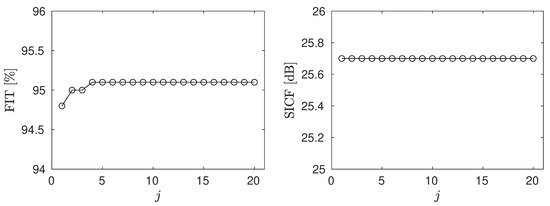
Figure 7. Convergence of the average FIT [%] and SICF [dB] values for the multi-step dfRLBF $[\mathrm{B},j]$ algorithm, evaluated for $k=100$ and $m=3$ at an SNR level of 10 dB over twenty iterations in the multi-step procedure ($j=1,\dots ,20$). The presented results were averaged over time for a single realization of the channel model (a typical example).

Figure 8 compares LBF, fLBF, and dfRLBF $[\mathrm{B},2]$ for $k=100$ and $m=3$ at an SNR level of 10 dB, focusing on parameter channel errors. The dfRLBF $[\mathrm{B},2]$ approach yields both quantitative and qualitative improvements over the LBF and fLBF algorithms. The improvement is noticeable for taps $i\ge 20$, where the channel parameter errors are smaller than in the other compared methods.

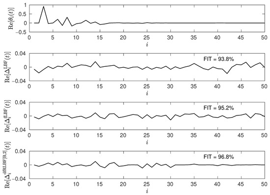
Figure 8. A snapshot of the true impulse response of the identified system (top figure) and three corresponding parameter channel errors obtained using the LBF, fLBF, and dfRLBF $[\mathrm{B},2]$, respectively, for $k=100$ and $m=3$ settings at an SNR level of 10 dB.

3.5. Impact of Measurement Noise

So far, it has been assumed that the measurement noise follows a Gaussian distribution. To provide a more comprehensive evaluation, three additional noise models are considered using the same experimental setup: Laplacian noise, non-stationary noise, and pulse noise. All noises meet the assumption ($\mathcal{A}$2).

The Laplacian noise is generated with the same variance as the Gaussian noise used in previous experiments [40]. This model is commonly employed to represent measurement noise that occasionally includes small outliers, as the heavier tails of the Laplace distribution make such deviations more likely compared to the Gaussian case.

To simulate non-stationary measurement noise, the noise variance was modulated over time according to the function

$$\begin{array}{c}\hfill {\sigma }_e\left(t\right)=0.7+0.5sin\left({\displaystyle \frac{2\pi t}{T}}\right)\end{array}$$

(88)

where T is the total number of samples. At each time instant, the noise sample was drawn from a zero-mean Gaussian distribution with the corresponding time-varying standard deviation $\mathcal{N}(0,{\sigma }_e^2\left(t\right))$.

Pulse noise is introduced using a Gaussian mixture model with $ϵ$-contamination [41]. Such a model is often used to describe measurement noise that is mostly Gaussian, but occasionally includes outliers or impulsive disturbances modeled by the high-variance Gaussian component. In this model, the noise distribution is a weighted sum (mixture) of two zero-mean Gaussian distributions with different variances

$$\begin{array}{c}\hfill p\left(x\right)=(1-ϵ),\mathcal{N}(0,{\sigma }_e^2)+ϵ,\mathcal{N}(0,\kappa {\sigma }_e^2)\end{array}$$

(89)

where $ϵ,(0<ϵ<1)$ denotes the probability that a sample is drawn from the contaminating distribution, determining the frequency of outliers, while the coefficient $\kappa \gg 1$ controls the severity of these outliers by substantially increasing the variance of the contaminated component.

Three realizations of measurement noise sequences with different distributions are presented in Figure 9. From to top to bottom: (A) Laplace noise, (B) non-stationary noise, and (C) pulse noise generated for parameters $\kappa =100,ϵ=0.01$. Table 4 presents the average FIT [%] and SICF [dB] values for the dfLBF and dfRLBF $\left[\mathrm{B}\right]$ algorithms under various types of measurement noise and at SNR levels of 10 dB, 20 dB, and 30 dB. Both approaches achieve high values for these metrics when applied to Gaussian, Laplacian, and non-stationary noise. However, performance drops significantly in the presence of pulse noise, primarily because the fLBF approach relies on ${\mathit{\ell }}^2$-norm minimization, which is not robust to impulsive disturbances. Nevertheless, under these challenging conditions, the dfRLBF $\left[\mathrm{B}\right]$ algorithm demonstrates a marked improvement over the dfLBF method. Similar results were also observed for the dfRLBF $\left[\mathbf{A}\right]$ and dfRLBF $\left[\mathrm{C}\right]$ approaches.

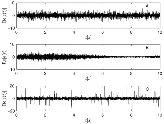
Figure 9. Three measurement noise sequences with different distributions. From top to bottom: (A) Laplacian noise, (B) non-stationary noise with time-varying variance, and (C) mixture noise—Gaussian noise contaminated by occasional impulsive (pulse) noise modeled for parameters $\kappa =100,ϵ=0.01$.

One practical solution is to incorporate a pulse detection algorithm that identifies pulses within the estimation window. With this enhancement, a robust LBF and fLBF approach would estimate channel parameters using only the outlier-free observations $y\left(t\right)$, as proposed in [42]. However, a limitation of this approach is that the estimation window will contain fewer data points, which, in cases of a high percentage of contamination, may lead to a drop in estimation performance or even numerical issues. An alternative solution, described in [43], combines pulse detection with the reconstruction of corrupted signal samples based on a signal model. This recursive algorithm is computationally efficient, preserves the original number of data points in the estimation window after reconstruction, and can effectively handle bursts of outliers affecting multiple consecutive samples. The results obtained by combining the pulse removal algorithm [43] with the proposed approaches are denoted as ‘Pulse*’ in Table 4. The pulse removal algorithm [43] based on semi-causal detection was configured with the following settings: an estimation window size of 201, a fifth-order AR model, a prediction-based detection threshold of 3.5, an interpolation-based detection threshold of 4.0, and a maximum detection burst length of 5.

Table 4. Average FIT [%] and SICF [dB] values for the dfLBF and dfRLBF [B] algorithms under various types of measurement noise—Gaussian noise, Laplacian noise, non-stationary noise, pulse noise, and data preprocessed with the pulse removal algorithm [43] (denoted as Pulse*). Performance was evaluated for parameters $k=300$ and $m=3$, across SNR levels of 10 dB, 20 dB, and 30 dB.

		FIT [%]			SICF [dB]
Method	Noise	10 dB	20 dB	30 dB	10 dB	20 dB	30 dB
dfLBF	Gaussian	93.3	97.7	98.8	26.4	35.6	41.5
	Laplace	92.5	97.4	97.4	25.8	35	33.3
	Non-stationary	91.8	97	97	23.8	33	34.4
	Pulse	65	66.3	66.4	10.3	10.5	10.6
	Pulse*	87	90.7	91.2	18.9	21.2	21.6
dfRLBF [B]	Gaussian	95.3	98.3	98.9	29.2	37.7	41
	Laplace	95.1	98.1	97.4	28.8	37	33.3
	Non-stationary	94.7	97.8	97.5	27.1	35.1	34.4
	Pulse	79.2	80	80.1	14.5	14.8	14.8
	Pulse*	91.8	93.9	94.3	22.5	24.6	24.9

Table 4. Average FIT [%] and SICF [dB] values for the dfLBF and dfRLBF [B] algorithms under various types of measurement noise—Gaussian noise, Laplacian noise, non-stationary noise, pulse noise, and data preprocessed with the pulse removal algorithm [43] (denoted as Pulse*). Performance was evaluated for parameters $k=300$ and $m=3$, across SNR levels of 10 dB, 20 dB, and 30 dB.

		FIT [%]			SICF [dB]
Method	Noise	10 dB	20 dB	30 dB	10 dB	20 dB	30 dB
dfLBF	Gaussian	93.3	97.7	98.8	26.4	35.6	41.5
	Laplace	92.5	97.4	97.4	25.8	35	33.3
	Non-stationary	91.8	97	97	23.8	33	34.4
	Pulse	65	66.3	66.4	10.3	10.5	10.6
	Pulse*	87	90.7	91.2	18.9	21.2	21.6
dfRLBF [B]	Gaussian	95.3	98.3	98.9	29.2	37.7	41
	Laplace	95.1	98.1	97.4	28.8	37	33.3
	Non-stationary	94.7	97.8	97.5	27.1	35.1	34.4
	Pulse	79.2	80	80.1	14.5	14.8	14.8
	Pulse*	91.8	93.9	94.3	22.5	24.6	24.9

3.6. Comparison with the Orthogonal Matching Pursuit

The Orthogonal Matching Pursuit (OMP) algorithm [24] was employed to obtain a sub-optimal least squares estimate of the hyperparameter vector $\mathbf{\alpha }$, as defined in (9). This estimation was achieved by selecting $N_{\mathrm{OMP}}$ most significant atoms. The atom dictionary, an $n(2k+1)\times nm$ matrix $\mathbf{F}$, was constructed from basis functions and explicitly defined as $\mathbf{F}={[{\mathbf{F}}^{\mathrm{T}}(-k),\dots ,{\mathbf{F}}^{\mathrm{T}}\left(k\right)]}^{\mathrm{T}}$. The corresponding observation vector, with dimensions $n(2k+1)\times 1$, was formed by concatenating all pre-estimate vectors, specifically ${[{\tilde{\mathit{\theta }}}_1^{\mathrm{T}}(t-k),\dots ,{\tilde{\mathit{\theta }}}_n^{\mathrm{T}}(t+k)]}^{\mathrm{T}}$.

A significant reduction in computational cost during the atom selection step is attributed to the sparse nature of matrix $\mathbf{F}$, characterized by its relatively small number of non-zero elements—only 2%. Furthermore, the block diagonal structure of $\mathbf{F}\left(j\right)$ provides crucial optimization for the OMP algorithm. This structure ensures that only a single coefficient needs to be determined per iteration, thereby avoiding the computationally intensive process of recomputing all previously identified coefficients, which is characteristic of standard OMP. This optimized implementation, while preserving the accuracy of the results, effectively lowers the computational cost of the OMP algorithm roughly by a factor of 12 compared to conventional OMP implementation. Additionally, once the atom dictionary is constructed with the chosen design parameters n, k, and m, it remains fixed throughout the simulation.

The atom dictionary for OMP algorithm was constructed with design parameters $n=50$, $k=100$, and $m=3$ to investigate the impact of the number of selected atoms on processing time. Table 5 summarizes the average FIT [%], SICF [dB], and processing time (${\mathrm{T}}_{\mathrm{p}}$ in seconds) achieved by OMP. This table illustrates how $N_{\mathrm{OMP}}$ (selected from $mn$ dictionary elements) influences performance under different SNR conditions (10 dB, 20 dB, 30 dB). The reported ${\mathrm{T}}_{\mathrm{p}}$ is for a single realization of 12,000-sample channel coefficients. In comparison, the dRLBF [B ] algorithm requires about 5 s for coefficient shrinking on the same CPU, after its regularization gains ($\eta$, $\mu$) are chosen, with their optimization taking roughly 68 s.

Table 5. Average FIT [%], SICF [dB] values, and processing time (${\mathrm{T}}_{\mathrm{p}}$) in seconds for the Orthogonal Matching Pursuit (OMP) algorithm. The table demonstrates the impact of the number of selected atoms ($N_{\mathrm{OMP}}$, chosen from $m\times n$ possible atoms in the dictionary) on performance across various SNR levels (10 dB, 20 dB, 30 dB). Processing time is measured per one realization of channel coefficients of length 12,000 samples. The best results per SNR level are indicated in bold.

		FIT [%]			SICF [dB]
${\mathbf{N}}_{\mathrm{OMP}}$	${\mathrm{T}}_{\mathrm{p}}$ [s]	10 dB	20 dB	30 dB	10 dB	20 dB	30 dB
10	128	91	91.9	92	22.4	23.2	23.4
20	230	93.5	96.8	97.4	26.2	32	33.3
30	327	92.2	96.6	97.5	25.1	32.2	34.4
40	431	91.3	96.4	97.3	24.3	31.9	34.5
50	528	90.7	96.1	97.2	23.9	31.6	34.5

It is important to note that an increasing number of selected atoms leads to a substantial increase in processing time, making the OMP algorithm less usable compared to the dfRLBF [B] approach for sliding window estimation. Furthermore, an increased number of atoms leads to a noticeable degradation in the OMP algorithm’s performance across both metrics, particularly evident at a low SNR of 10 dB—see Figure 10. At higher SNR levels (20 dB and 30 dB), this degradation remains observable but is smaller.

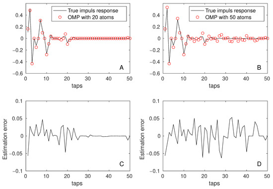
Figure 10. A snapshot of the true impulse response (solid line) and superimposed OMP estimates (circles) for $N_{\mathrm{OMP}}=20$ and $N_{\mathrm{OMP}}=50$ atoms are shown in Plots (A) and (B), respectively. OMP results were generated under parameters $k=100$ and $m=3$ at an SNR of 10 dB. Plots (C,D), directly below, illustrate the parameter estimation errors corresponding to the OMP results presented in Plots (A,B).

Table 6 presents the average FIT [%] and SICF [dB] values achieved by the OMP algorithm at different SNR levels (10 dB, 20 dB, and 30 dB), using a fixed selection of $N_{\mathrm{OMP}}=20$ atoms. For each experimental condition, atom dictionaries were constructed from matrices $\mathbf{F}\left(j\right),j\in [-k,k]$, utilizing a fixed $n=50$ and exploring all combinations of $k\in [100,300]$ and $m\in [1,3,5]$. At a low SNR of 10 dB, the OMP algorithm achieved the best results among the evaluated methods (LBF, fLBF, dfLBF). Only the dfRLBF [B] approach yielded performance comparable to OMP at this SNR level. Conversely, for SNR values of 20 dB and 30 dB, dfRLBF [B] demonstrated superior performance over OMP, with this advantage becoming more pronounced as the SNR increased. Table 7 shows average $\Delta$FIT [%] and $\Delta$SICF [dB] values, showing the difference in scores between the dfRLBF [B] and OMP algorithms. Positive values indicate dfRLBF [B]’s superior performance, whereas negative values suggest OMP’s better performance.

Table 6. Average FIT [%] and SICF [dB] values for the Orthogonal Matching Pursuit (OMP) algorithm, using $N_{\mathrm{OMP}}=20$ selected atoms. For these experiments, atom dictionaries were constructed from matrices $\mathbf{F}\left(j\right),j\in [-k,k]$ for each combination of design parameters: fixed $n=50$, $k\in [100,300]$, and $m\in [1,3,5]$. The best results per SNR level are indicated in bold.

		FIT [%]			SICF [dB]
SNR	k/m	1	3	5	1	3	5
10 dB	100	93.4	93.5	93.4	26.3	26.2	26.1
	300	90.49	95.3	95.2	22	28.2	28.3
20 dB	100	96.8	96.8	96.8	32.3	32	31.9
	300	91.2	96.5	96.4	22.4	31	30.7
30 dB	100	97.4	97.4	97.3	33.6	33.3	33.2
	300	91.2	96.6	96.5	22.5	31.3	31

Table 7. Average $\Delta$FIT [%] and $\Delta$SICF [dB] values, quantifying the performance difference between the dfRLBF [B] and OMP ($N_{\mathrm{OMP}}=20$ atoms) algorithms. The table illustrates the impact of varying design parameters: local estimation window size ($2k+1$, for $k\in [100,300]$) and number of basis functions ($m\in [1,3,5]$), across SNR levels of 10 dB, 20 dB, and 30 dB. Positive values indicate dfRLBF [B]’s superior performance, whereas negative values suggest OMP’s better performance.

		$\Delta$FIT [%]			$\Delta$SICF [dB]
SNR	k/m	1	3	5	1	3	5
10 dB	100	0.7	−0.8	−1.7	1.1	−0.4	−1.4
	300	0.71	0	−0.6	0.6	1	−0.2
20 dB	100	0.9	0.4	−0.1	2.8	1.9	0.9
	300	0.7	1.8	1.7	0.7	6.1	5.6
30 dB	100	1	0.8	0.4	3.9	3.4	2.4
	300	0.8	2.3	2.4	0.7	9.7	9.6

3.7. Discussion

Once the communication channel can be approximated by the time-varying FIR model shown in (1), the main goal is to identify the unknown time-varying system coefficients. The assumption regarding the speed of parameter changes is very important, as it determines the choice of the identification algorithm. Classical identification algorithms are typically limited to tracking slowly time-varying parameters [4,5,6]. In contrast, the time-varying channel identification algorithm proposed in this paper is designed to effectively track parameter variations at various speeds, including slow, medium, and fast changes. This enhanced capability is achieved through the use of a hypermodel based on local basis functions. By employing a linear combination of an appropriate number of basis functions (m) and selecting a suitable analysis window size (K), the algorithm can accurately capture even rapid parameter changes. Therefore, the design parameters m and K play a crucial role in the performance of the identification process, as demonstrated in all tables presented.

Previous research has proposed two local statistics for parameter selection: the cross-validation selection rule [29] and the modified Akaike’s final prediction error criterion [39]. In this paper, we show that the cross-validation selection rule is also effective for the proposed regularized estimators. As shown in Table 2, results obtained using this rule closely approach the best results across all tested combinations of m and k. Recent works [44,45] show that if there is prior knowledge of parameter changes, it can improve the selection and/or type of basis functions used in the local basis function approach.

Another important aspect examined in this work is the compensation of estimation bias introduced by the causal EWLS algorithm used to obtain pre-estimates at the first stage. This bias can be mitigated by replacing unidirectional pre-estimates with bidirectional pre-estimates. Alternatively, as detailed in Equations (79)–(82), the parameter estimates can also be refined by applying a time-shift correction at each time instant. As shown in Table 1, the time-shift correction leads to improved estimation results across all SNR cases, with greater benefits observed at higher SNR levels. However, accurately estimating the time-shift in low SNR scenarios remains challenging and may require further investigation in future research.

Next, it was demonstrated that the proposed regularization technique is suitable for channel identification with sparse characteristics. As shown in Figure 8, the channel parameter errors are reduced and are closer to zero in the impulse response tail compared to the LBF or fLBF methods. This behavior is the expected outcome of the proposed method. To achieve the best results, it is necessary to select the regularization gains adaptively. In this paper, three gain selection approaches were derived and compared. The best results were obtained when the gain selection was performed independently for each system coefficient.

The proposed method was validated using various noise models, including Gaussian noise, Laplace noise, non-stationary noise, and pulse noise, achieving high estimation accuracy for all cases except the challenging pulse noise scenario (see Table 4). Since both the LBF and fLBF approaches are based on ${\mathit{\ell }}^2$-norm minimization, they are inherently not robust to severe impulsive (pulse) noise. Even a small proportion of contamination, such as 1%, can significantly degrade the accuracy of channel parameter estimation. To address this challenge, an additional preprocessing step can be implemented to detect and exclude, trim, or replace corrupted samples before applying the proposed method, as discussed in [42]. Alternatively, the strategy proposed in [43] allows for detecting corrupted samples and replacing them with interpolated values based on a signal model.

Finally, the proposed approach was compared with the Orthogonal Matching Pursuit (OMP) algorithm [24]. The atom dictionary, constructed from basis functions, exhibited inherent sparsity and a block diagonal structure, which reduced the computational cost of the OMP algorithm by a factor of 12 without affecting its results. Nevertheless, the computational burden of OMP remained significantly higher than that of the dfRLBF [B] approach, and was strongly dependent on the number of selected atoms. While OMP achieved comparable results to dfRLBF [B] with 20 atoms at a low SNR of 10 dB, its performance in both metrics declined at higher SNR levels (20 dB and 30 dB).

A brief summary of the key aspects of the proposed multistage method for non-stationary sparse channel identification is provided in Table 8.

Table 8. Summary of proposed multistage approach for identification of non-stationary sparse communication channels.

Aspect	Description
Goal	Identification of non-stationary communication channels exhibiting sparsity, approximated by an FIR model.
Estimation framework	Sliding window approach with model parameters updated at each time instant.
Rate of channel variation	Tracks slow, medium, and fast variations; no assumption of local stationarity.
Algorithm features	Approximated closed-form solution; computationally efficient, recursive, adaptive, and does not require matrix inversion.
Numerical stability	Recursive fLBF algorithm is marginally stable; periodic reset required (e.g., every 1000 steps).
Measurement noise	Validated using various noise models, including Gaussian, Laplacian, non-stationary, and pulse noise. High estimation accuracy achieved in all cases except for pulse noise; robustness can be enhanced by excluding or interpolating corrupted samples (see [42,43]).
Sparse problems	Handles sparse systems using two reweighted ${\mathit{\ell }}^2$ regularizers; both regularization gains are adaptively optimized at each time instant.
Multistage method	Yes (three stages).
Stage 1	The pre-estimates are obtained using inverse filtering of EWLS estimates or, for reduced cost, the iterative dichotomous coordinate descent algorithm; followed by fLBF estimation with adaptive hyperparameter selection (e.g., number of basis functions, window size, decay profile).
Stage 2	fRLBF estimation with joint or separate optimization of regularization gains for each fLBF estimate.
Stage 3	Multi-step refinement procedure with a few iterations to further improve fRLBF estimates.

4. Conclusions

The proposed regularization technique, using local basis functions with reweighted ${\mathit{\ell }}^2$ regularizers in both the time and frequency domains, effectively enhances the identification of non-stationary communication channels, especially those with sparse characteristics and exponential envelope profiles, as commonly observed in full-duplex underwater acoustic channels. Three adaptive gain selection approaches, the empirical Bayes, decentralized, and cross-validation, were investigated, showing additional improvements with debiasing and multi-step procedures. The proposed fRLBF approach presents a superior alternative to LBF for lower SNR levels (10 and 20 dB), providing lower complexity and greater flexibility. In simulation experiments, the proposed fRLBF approach achieved results that were competitive with, or even superior to, those obtained using the Orthogonal Matching Pursuit algorithm, while also delivering significant computational savings. Additionally, the proposed method demonstrated robustness to various types of measurement noise—including Gaussian, Laplacian, and non-stationary noise—but its performance deteriorated in the presence of pulse noise. This suggests that a preprocessing step for pulse noise removal should be considered in such scenarios.

References

- Tsatsanis, M.K.; Giannakis, G.B. Modeling and equalization of rapidly fading channels. Int. J. Adapt. Contr. Signal Process. 1996, 10, 159–176. [Google Scholar] [CrossRef]
- Stojanovic, M.; Preisig, J. Underwater acoustic communication channels: Propagation models and statistical characterization. IEEE Commun. Mag. 2009, 47, 84–89. [Google Scholar] [CrossRef]
- Songzuo, L.; Iqbal, B.; Khan, I.U.; Ahmed, N.; Qiao, G.; Zhou, F. Full Duplex Physical and MAC Layer-Based Underwater Wireless Communication Systems and Protocols: Opportunities, Challenges, and Future Directions. J. Mar. Sci. Eng. 2021, 9, 468. [Google Scholar] [CrossRef]
- Söderström, T.; Stoica, P. System Identification; Prentice-Hall: Hoboken, NJ, USA, 1988; ISBN 978-0-13-881236-2. [Google Scholar]
- Haykin, S. Adaptive Filter Theory; Prentice-Hall: Hoboken, NJ, USA, 1996; ISBN 978-0-13-322760-4. [Google Scholar]
- Niedźwiecki, M. Identification of Time-Varying Processes; Wiley: Hoboken, NJ, USA, 2000; ISBN 978-0-471-98629-4. [Google Scholar]
- Kitagawa, G.; Gersch, W. A smoothness priors time-varying AR coefficient modeling of nonstationary covariance time series. IEEE Trans. Autom. Control 1985, 30, 48–56. [Google Scholar] [CrossRef]
- Kitagawa, G.; Gersch, W. Smoothness Priors Analysis of Time Series; Springer: Berlin/Heidelberg, Germany, 1996; ISBN 978-0-387-94819-5. [Google Scholar]
- Niedźwiecki, M. Locally adaptive cooperative Kalman smoothing and its application to identification of nonstationary stochastic systems. IEEE Trans. Signal Process. 2012, 60, 48–59. [Google Scholar] [CrossRef]
- Niedźwiecki, M. Functional series modeling approach to identification of nonstationary stochastic systems. IEEE Trans. Autom. Control 1988, 33, 955–961. [Google Scholar] [CrossRef]
- Tsatsanis, M.K.; Giannaki, G.B. Time-varying system identification and model validation using wavelets. IEEE Trans. Signal Process. 1993, 41, 3512–3523. [Google Scholar] [CrossRef]
- Borah, D.K.; Hart, B.D. Frequency-selective fading channel estimation with a polynomial time-varying channel model. IEEE Trans. Commun. 1999, 47, 862–873. [Google Scholar] [CrossRef]
- Wei, H.L.; Liu, J.J.; Billings, S.A. Identification of time-varying systems using multi-resolution wavelet models. Int. J. Syst. Sci. 2002, 33, 1217–1228. [Google Scholar] [CrossRef]
- Niedźwiecki, M.; Ciołek, M. Generalized Savitzky-Golay filters for identification of nonstationary systems. Automatica 2020, 108, 108477. [Google Scholar] [CrossRef]
- Ljung, L.; Chen, T. What can regularization offer for estimation of dynamic systems? In Proceedings of the 11th IFAC Workshop on Adaptation and Learning in Control and Signal Processing, Caen, France, 3–5 July 2013; pp. 1–8. [Google Scholar]
- Chen, T.; Ohlsson, H.; Ljung, L. On the estimation of transfer functions, regularizations and Gaussian process—Revisited. Automatica 2012, 48, 1525–1535. [Google Scholar] [CrossRef]
- Pillonetto, G.; Dinuzzo, F.; Chen, T.; De Nicolao, G.; Ljung, L. Kernel methods in system identification, machine learning and function estimation: A survey. Automatica 2014, 50, 657–682. [Google Scholar] [CrossRef]
- Gańcza, A.; Niedźwiecki, M.; Ciołek, M. Regularized local basis function approach to identification of nonstationary processes. IEEE Trans. Signal Process. 2021, 69, 1665–1680. [Google Scholar] [CrossRef]
- Niedźwiecki, M.; Gańcza, A.; Kaczmarek, P. Identification of fast time-varying communication channels using the preestimation technique. In Proceedings of the 19th Symposium on System Identification, SYSID, Padova, Italy, 13–16 July 2021; Volume 54, pp. 351–356. [Google Scholar]
- Tibshirani, R. Regression shrinkage and selection via the LASSO. J. R. Statist. Soc. B 1996, 58, 267–288. [Google Scholar] [CrossRef]
- Tipping, M.E. Sparse Bayesian Learning and the Relevance Vector Machine. J. Mach. Learn. Res. 2001, 1, 211–244. [Google Scholar]
- Daubechies, I.; Defrise, M.; De Mol, C. An iterative thresholding algorithm for linear inverse problems with a sparsity constraint. Commun. Pure Appl. Math. 2004, 57, 1413–1457. [Google Scholar] [CrossRef]
- Beck, A.; Teboulle, M. A Fast Iterative Shrinkage-Thresholding Algorithm for Linear Inverse Problems. SIAM J. Imaging Sci. 2009, 2, 183–202. [Google Scholar] [CrossRef]
- Davis, G.; Mallat, S.; Avellaneda, M. Adaptive greedy approximations. Constr. Approx. 1997, 13, 57–98. [Google Scholar] [CrossRef]
- Needell, D.; Tropp, J.A. Iterative signal recovery from incomplete and inaccurate samples. Appl. Comput. Harmon. Anal. 2009, 26, 301–321. [Google Scholar] [CrossRef]
- Boyd, S.; Parikh, N.; Chu, E.; Peleato, B.; Eckstein, J. Distributed Optimization and Statistical Learning via the Alternating Direction Method of Multipliers. Found. Trends® Mach. Learn. 2011, 3, 1–122. [Google Scholar] [CrossRef]
- Gańcza, A.; Niedźwiecki, M. Regularized identification of fast time-varying systems—Comparison of two regularization strategies. In Proceedings of the 60th IEEE Conference on Decision and Control, Austin, TX, USA, 14–17 December 2021; pp. 864–871. [Google Scholar]
- Shen, L.; Zakharov, Y.; Henson, B.; Morozs, N.; Mitchell, P. Adaptive filtering for full-duplex UWA systems with time-varying self-interference channel. IEEE Access 2020, 8, 187590–187604. [Google Scholar] [CrossRef]
- Niedźwiecki, M.; Ciołek, M.; Gańcza, A. A new look at the statistical identification of nonstationary systems. Automatica 2020, 118, 109037. [Google Scholar] [CrossRef]
- Niedźwiecki, M.; Gańcza, A.; Ciołek, M. On the preestimation technique and its application to identification of nonstationary systems. In Proceedings of the 59th Conference on Decision and Control CDC 2020, Jeju Island, Republic of Korea, 14–18 December 2020; pp. 286–293. [Google Scholar]
- Zakharov, Y.V.; White, G.P.; Liu, J. Low-complexity RLS algorithms using dichotomous coordinate descent iterations. IEEE Trans. Signal Process. 2008, 56, 3150–3161. [Google Scholar] [CrossRef]
- Friedman, J.; Hastie, T.; Tibshirani, R. A note on the group lasso and sparse group lasso. arXiv 2010, arXiv:1001.0736. [Google Scholar] [CrossRef]
- Bani, M.S.; Chalmers, B.L. Best approximation in Linf via iterative Hilbert space procedures. J. Approx. Theory 1984, 42, 173–180. [Google Scholar] [CrossRef]
- Burrus, C.S.; Barreto, J.A.; Selesnick, I.W. Iterative reweighted least squares design of FIR filters. IEEE Trans. Signal Process. 1994, 42, 2926–2936. [Google Scholar] [CrossRef]
- Gańcza, A. Local Basis Function Method for Identification of Nonstationary Systems. Ph.D. Thesis, The Gdańsk University of Technology, Gdańsk, Poland, 2024. [Google Scholar]
- Good, I.J. The Estimation of Probabilities; MIT Press: Cambridge, MA, USA, 1965; ISBN 978-0-262-57015-2. [Google Scholar]
- Niedźwiecki, M.; Gańcza, A.; Shen, L.; Zakharov, Y. Adaptive identification of linear systems with mixed static and time-varying parameters. Signal Process. 2020, 200, 108664. [Google Scholar] [CrossRef]
- Niedźwiecki, M.; Gańcza, A.; Shen, L.; Zakharov, Y. On Bidirectional preestimates and their application to identification of fast time-varying systems. In Proceedings of the IEEE International Conference on Acoustics, Speech and Signal Processing (ICASSP), Rhodes Island, Greece, 4–10 June 2023; pp. 1–5. [Google Scholar]
- Niedźwiecki, M.; Ciołek, M. Fully adaptive Savitzky-Golay type smoothers. In Proceedings of the 27th European Signal Processing Conference (EUSIPCO), A Coruna, Spain, 2–6 September 2019; pp. 1–5. [Google Scholar]
- Miller, S.L.; Childers, D.G.S. Probability and Random Processes: With Applications to Signal Processing and Communications, 2nd ed.; Academic Press: Cambridge, MA, USA, 2012; ISBN 978-0-12-386981-4. [Google Scholar]
- Huber, P.J. Robust Estimation of a Location Parameter. Ann. Math. Stat. 1964, 35, 73–101. [Google Scholar] [CrossRef]
- Niedźwiecki, M.; Gańcza, A.; Żuławiński, W.; Wyłomańska, A. Robust local basis function algorithms for identification of time-varying FIR systems in impulsive noise environments. In Proceedings of the 63rd Conference on Decision and Control (CDC), Milan, Italy, 16–19 December 2024; pp. 3463–3470. [Google Scholar]
- Ciołek, M.; Niedźwiecki, M. Detection of impulsive disturbances in archive audio signals. In Proceedings of the 2017 IEEE International Conference on Acoustics, Speech and Signal Processing (ICASSP), New Orleans, LA, USA, 5–9 March 2017; pp. 671–675. [Google Scholar]
- Niedźwiecki, M.; Gańcza, A. Karhunen-Loeve-based approach to tracking of rapidly fading wireless communication channels. Signal Process. 2023, 209, 109043. [Google Scholar] [CrossRef]
- Niedźwiecki, M.; Gańcza, A. On Optimal Tracking of Rapidly Varying Telecommunication Channels. IEEE Trans. Signal Process. 2024, 72, 2726–2738. [Google Scholar] [CrossRef]
Disclaimer/Publisher’s Note: The statements, opinions and data contained in all publications are solely those of the individual author(s) and contributor(s) and not of MDPI and/or the editor(s). MDPI and/or the editor(s) disclaim responsibility for any injury to people or property resulting from any ideas, methods, instructions or products referred to in the content. |
© 2025 by the author. Licensee MDPI, Basel, Switzerland. This article is an open access article distributed under the terms and conditions of the Creative Commons Attribution (CC BY) license (https://creativecommons.org/licenses/by/4.0/).