Air Quality Prediction Affected by Different Activation Functions and Hidden Layer Nodes in Artificial Neural Network Models

Abstract

The effects of different activation functions (sigmoid and hyperbolic tangent), and node numbers in a hidden layer of artificial neural network (ANN) models on urban air quality forecasting were investigated in a coastal city of Korea. The ANN models of multilayer perceptron (MLP) with a back-propagation training algorithm for error calculation in cases of 13, 15, and 17 nodes in each hidden layer were performed using 15 input independent variables (PM, gas, and meteorological data of Gangneung city (Republic of Korea)), affected by PM and gas of an upwind Beijing city (China). Root mean square error (RMSE) and the coefficient of determination (R²; Pearson R) were evaluated to assess the two models’ forecasting abilities between the predicted and measured values. The values of R by ANN-sig (ANN-tanh) with 13, 15, and 17 hidden neuron numbers were 0.930 (0.950), 0.920 (0.947), 0.926(0.953) on PM₁₀, 0.953 (0.956), 0.927 (0.938), 0.949 (0.960) on PM_2.5, and 0.880 (0.959), 0.917 (0.886), and 0.882 (0.939) on NO₂. Regardless of node numbers and activation functions, the prediction abilities of the two models were excellent, showing the highest values of R in the ANN-tanh model with more neuron numbers in the hidden layer. Unlike previous studies’ insistence that smaller nodes (larger) in the hidden layer produce the overfit (underfit) result in the ANN model, the present study proves that more nodes in its hidden layer than the input layer can yield the best prediction than any other, as shown in their temporal distributions and scatter plots of predicted and measured data. Future-time air quality forecasting at Gangneung city can be calculated sequentially using its current time data and previous time data from Beijing city, using the suggested empirical formulas.

1. Introduction

The previous research explained that severe air pollution of particulate matter associated with gaseous (SO₂, CO, NO₂, and O₃) due to the traffic vehicles on the road, the subway trains, and the large rural urbanization, and frequent forest, farm, and residential fires and the influx of Chinese yellow dust causes not only very harmful to the human body with respiratory disease and outdoor physical activity, but also reduces visibility [1,2,3,4,5,6,7,8,9].

In spring, when the yellow dust in spring occurs under a wind speed of over 10 m/s and a relative humidity of less than 40% in the air near the surface of the dry land and desert, such as the Gobi Desert, the Kubuchi Desert, the Loess Plateau, and even the Taklimakan Desert in Mongolia and China, a huge amounts of yellow dust raised from the ground surface flow up to 3 km or 5 km height, and they are vertically and horizontally transported to the widely downwind regions of the eastern China, Korea, Japan, Taiwan, and southern Asian countries, causing severe high PM and gas concentrations associated with local meteorological condition and atmospheric boundary layer [10,11,12,13,14,15,16,17].

Three dimensional numerical modeling research for air pollutant dispersion including photo-chemical reaction processes and particle transportation has been carried by Kotamarthi and Carmichael [18], David et al. [19], Lin [20], McKendry et al. [21], Uno et al. [22], Jeong et al. [23], and Kong et al. [24] under a long-range transport of Asian Dust from the source regions of the deserts and arid areas in northern China to eastern China, Taiwan, Korea, Japan, southern California, and Canada. The advantage of numerical modeling is to show the three-dimensional air pollutant distribution in detail, but the disadvantage is that it requires many input data and CPU time for the model operation, making it expensive.

In recent decades, many researchers like Li et al. [25], Kim [26], Choi and Choi [27], and Choi et al. [17] have used multivariate statistical regression techniques instead of a simple regression model for predicting particulate matter and gas concentrations affected by meteorological parameters in various ways. Their prediction abilities supply quite accurate results close to the measured data, though those models consist of relatively simple algorithms rather than numerical models.

Since Masters [28] and Shahin et al. [29] used artificial neural network (ANN) techniques, many scientists have applied these techniques to predict air quality, due to yellow dust, fugitive dust, soil-driven dust, and the COVID-19 pandemic [30,31,32]. Jeon and Son [33] predicted daily mean PM₁₀ concentration in Seoul by ANN-sigmoid, Support Vector Machine (SVM), and Random Forest (RF) models, with a low Pearson R of 0.726~0.75. Lee and Lee [34] showed hourly mean PM_2.5 concentration by ANN-sigmoid, LSTM (long short-term memory), and RF techniques with the R of 0.837, 0.907, and 0.910, and Choi [35] predicted hourly mean PM₁₀, PM_2.5, and NO₂ concentrations by the ANN-tanh model and multivariate regression model with the high R of 0.909~0.977, except for 0.853~0.925 for NO₂ in Korea by the trans-boundary Chinese air pollutants.

Their ANN model performances had lower computational complexity and shorter computation time than the numerical models and produced very good results. Unfortunately, it is not easy to find research articles that quantify the extent of the effect of different node numbers in the hidden layer of the ANN associated with different activation functions on air quality forecasting. Roy [36] mentioned without any detailed information that smaller nodes (larger) in the hidden layer produce the overfit (underfit) result in the ANN model.

Thus, the main purpose of this study is to verify how the different node numbers in the hidden layer of the ANN associated with different activation functions can affect the current air quality forecasting at a Korean city, using 3 h earlier PM, gases, and meteorological elements, affected by the 48 h earlier trans-boundary PM, and gases from China. Root mean square errors (RMSE) and determination coefficients (R²) were calculated to assess the prediction accuracy of two ANN models, and the results were compared by plotting the hourly distributions and scatter plots with empirical formulas for the predicted and measured values of output variables.

2. Study Area and Data Analysis

2.1. Site Description

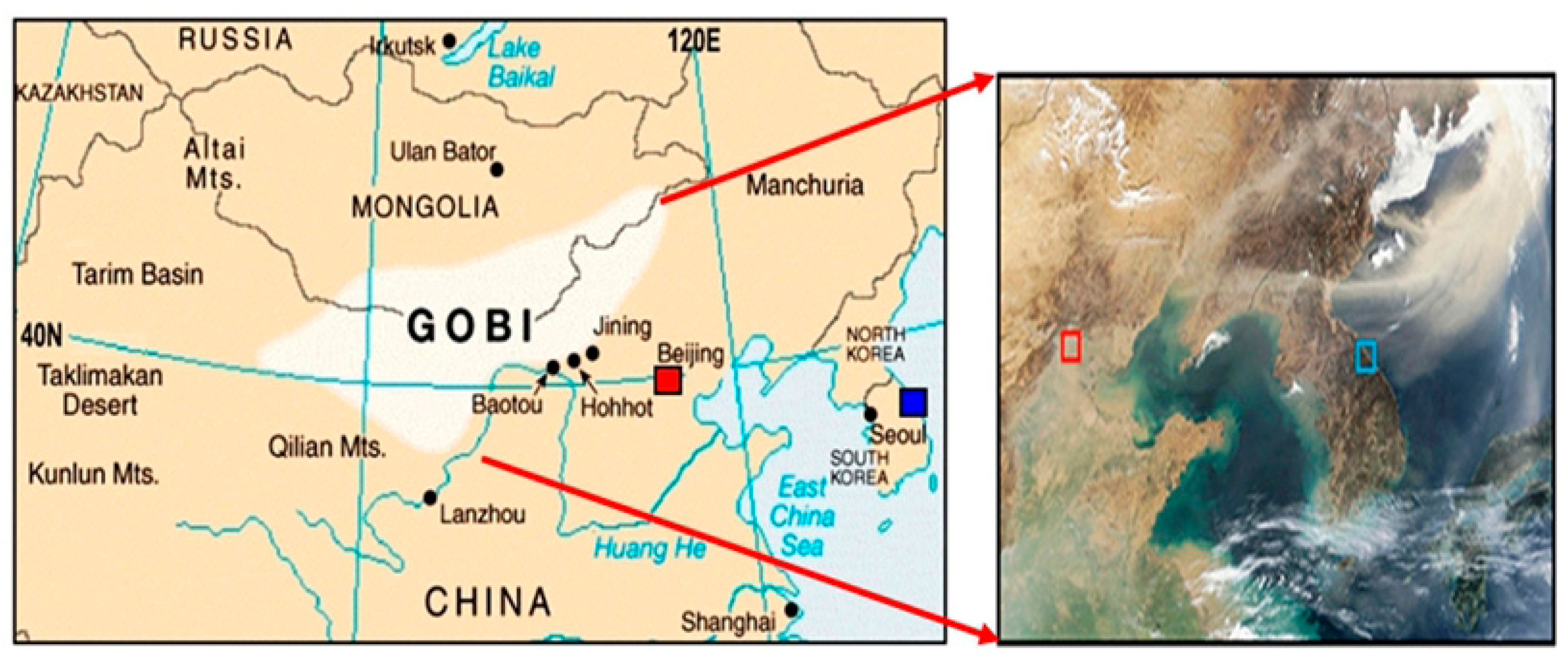
The study area (Gangneung city; 37.751° N, 128.876° E) in the Republic of Korea is located in the coastal basin of a mean sea level of 25 m, surrounded by high mountains in the west and the Sea of Japan in the east (Figure 1). As the vehicles on the road and boilers for cooking and heating in the apartment in this city with no industry are major air pollution sources, its air quality is very good, more or less than 40 μg/m³ of PM₁₀ [27].

Figure 1. Map of Asia (left: Mongolia, northern China, and Republic of Korea) and satellite dust images (right, thin yellow color). Red and blue squares denote Beijing city (China) and Gangneung city (Republic of Korea). (https://kr.pinterest.com/pin/gobi-desert-map--269371621436682946/ (accessed on 15 January 2024). https://visibleearth.nasa.gov/images/58069/dust-over-korea-and-the-sea-of-japan (accessed on 15 January 2024)).

During the periods of strong northwesterly wind prevailing in the northeastern Asia of spring, a large amount of yellow dust from the Gobi Desert and arid northern China was transported to the downwind Chinese city (Beijing) and combined with its urban pollutants. Thereafter, those pollutants were further transported to the Korean peninsula and Japanese island, resulting in three times higher PM (PM₁₀, PM_2.5) and gas (SO₂, NO₂, CO, O₃) concentrations than normal air pollution state and worse visibility. A satellite image shows yellow dust raised from the Gobi Desert across China and the Korean peninsula of Gangneung city.

2.2. Data Acquisition and Analysis

In this study, hourly mean PM₁₀ and PM_2.5 concentrations were measured by an Ambient Air Particle Monitoring System (German product, GRIMM 1107, DURAG Group, Hamburg, Germany) at Myungjudong in Gangneung city (Republic of Korea), and hourly mean SO₂, NO₂, CO, and O₃ concentrations measured at Okchendong near Myungjudong by “the Gangwon Health and Environmental Research Institute (GHERI)” were obtained from “Air Korea of the Korea Environment Corporation” (Sejong-si, Republic of Korea (Ministry of Interior and Safety)) through a website (https://www.airkorea.or.kr/web/, accessed on 15 January 2024) [29]. Hourly meteorological data (air temperature (°C; Temp), wind speed (m/s; Wind), and relative humidity (%); RH) measured at “Myungjudong Meteorological Observatory of the Gangwon Regional Meteorological Administration (GRMA)” were obtained from “the Korea Meteorological Administration (KMA)” through a website (https://data.kma.go.kr/, accessed on 25 February 2024). All measuring stations in the downtown area of the city were adjacent to each other. Thus, 3 h earlier hourly PM (PM₁₀ and PM_2.5), gas (SO₂, CO, NO₂, O₃), and meteorological data in Gangneung city from 21:00 LST 22 March to 21:00 LST 26 March were used for forecasting Gangneung’s current air quality from 00:00 LST 23 March to 00:00 LST 27 March 2015.

Generally, in spring, a huge amount of yellow dust raised from the Gobi Desert by strong westerly winds is transported toward Beijing city and combined with urban pollutants emitted from its city. Thereafter, the combined pollutants further reach Gangneung city in Korea by approximately 8 m/s westerly wind across 1300 km for 48 h and recombine with its local pollutants, causing a severe air pollution state [12,15,22,24]. Thus, 48 h earlier hourly PM (PM₁₀ and PM_2.5) and gas (SO₂, CO, NO₂, and O₃) data of Nan-san-huan-lu measurement point in Beijing from 00:00 LST 21 March to 00:00 LST 25 March were used for forecasting Gangneung’s current air quality from 00:00 LST 23 March to 00:00 LST 27 March.

The air pollution data were obtained through a website (https://quotsoft.net/air/, accessed on 8 January 2024). A total of 1455 hourly data of 15 input variables (3 h before—9 variables at Gangneung city (PMs, gaseous, meteorological elements)—and 48 h before—6 variables at Beijing city (PMs, and gaseous)) were used for forecasting hourly PM₁₀, PM_2.5, and NO₂ output variables at Gangneung city using ANN-sigmoid and ANN-tanh models.

3. Artificial Neural Network Models

3.1. Artificial Neural Network Techniques with Sigmoid and Tanh Functions

Masters [28], Rumelhart et al. [37], Shahin et al. [29], Dhakal et al. [38], Roy [36], Choi and Choi [35], and Jaiswal [39] described well a feed-forward ANN model (sigmoid or tanh) as a multilayer perceptron (MLP), which is an artificial feedforward neural network comprising input layer, hidden layer, and output layer with a set of linked artificial neurons in each layer and with back-propagation training algorithm for error calculation between the predicted and measured values (Figure 2).

Figure 2. ANN’s topology of the MLP with 15 nodes in the input and hidden layers, and 3 nodes in the output layer, as a sample, but output data computed using the 13, 15, and 17 hidden nodes separately through the sigmoid and tanh functions were compared with the measured data to obtain an optimal model.

This topology shows the MLP with 15 nodes in input and hidden layers, and 3 nodes in the output layer as a sample case, but the ANN modeling process was taken with 13, 15, and 17 nodes in the hidden layer, considering separately, and then the models’ simulation results were compared. Table 1 denotes a total of 15 variables with 3 h earlier input data of 9 variables in Gangneung city (G) and 48 h earlier input data of 6 variables in Beijing (B) to be initially set in the input layer and calculated through sigmoid (tanh) activation function by multiplying a group of weights to each input data and the calculated each results were sent to the hidden layer.

Table 1. Definition of input and output variables in the ANN-sigmoid and ANN-tanh models. G and B indicate Gangneung (Republic of Korea) and Beijing (China).

Input Variable		Definition of Abbreviation		Output Variable
$x_1$	PM10-G	Particulate Matter < 10 um (μg/m3)	3 h before	$y_1$(31) PM10-G(F) $y_2$(32) PM2.5-G(F) $y_3$(33) NO2-G(F) at the forecasting time of Gangneung city
$x_2$	PM2.5-G	Particulate Matter < 2.5 um (μg/m3)
$x_3$	T-G	Air Temperature (°C)
$x_4$	W-G	Wind Speed (m/s)
$x_5$	RH-G	Relative Humidity (%)
$x_6$	SO2-G	Sulfur Dioxide (ppm)
$x_7$	CO-G	Carbon Monoxide (ppm)
$x_8$	NO2-G	Nitrogen Dioxide (ppm)
$x_9$	O3-G	Ozone (ppm)
$x_{10}$	PM10-B	Particulate Matter < 10 um (μg/m3)	48 h before
$x_{11}$	PM2.5-B	Particulate Matter < 2.5 um(μg/m3)
$x_{12}$	SO2-B	Sulfur Dioxide (ppm)
$x_{13}$	CO-B	Carbon Monoxide (ppm)
$x_{14}$	NO2-B	Nitrogen Dioxide (ppm)
$x_{15}$	O3-B	Ozone (ppm)

In the same kind of way, the each result by multiplying a set of new weights to each node in the hidden layer through another sigmoid (tanh) activation function were sent to the output layer, finally obtaining 3 desired output data of node number 31 to 33 as y₁(31) (PM_10-G(F)), y₂(32) (PM_2.5-G(F)), and y₃(33) (NO_2-G(F)). Both ANN-sigmoid and ANN-tanh modeling processes were performed with hourly independent variables as input data x_j (j = 1 to 15) for forecasting 3 dependent variables as final output data y_i (i = 1 to 3) using IBM SPSS v27 statistics software.

3.2. Training, Testing, and Validation of PM₁₀, PM_2.5, and NO₂ by ANN Models

The available data of 1455 as total hourly data for 4 days were divided into three groups, with the initial 60% of the total data randomly split for the training, 20% for the testing, and the remaining 20% for validation purposes for the ANN model development at Gangneung city. All data were scaled between 0 and 1 for the sigmoid activation function (−1 to 1 for the tanh activation function) to remove their dimension and to obtain equal attention by Equation (1) during training for the ANN-sigmoid (the ANN-tanh) model development.

For data scaling, the linear mapping of the variables’ practical extremes to the neural network’s practical extremes was adopted, similar to the suggestions by Masters [28], Shahin et al. [29], Nawras and Hani [31], and Choi [32]. The scaled value $x_n$ is calculated using each variable $x$ with the maximum and minimum values of $x_{max}$ and $x_{min}$, as in Equation (1).

$$x_n={\displaystyle \frac{\left(x-x_{min}\right)}{\left(x_{max}-x_{min}\right)}}$$

(1)

The output neurons j ($y_j$) in the MLP with 15 nodes in a single hidden layer are calculated by Equations (2)–(4) using sigmoid (or tanh) activation, and the final output neurons in the output layer ($y_{31}$, $y_{32},y_{33}$) are computed by the same activation function of sigmoid (or tanh), sequentially.

$$y_j=f \left({\theta }_j+{\sum }_{j=16}^p{w}_{i,j}{x}_i\right)$$

(2)

$$y_j=f\left(x\right)=sigmoid\left(x\right)={\displaystyle \frac{1 }{1+e^{-x}}}$$

(3)

$$y_j=f\left(x\right)=\tan \left(x\right)={\displaystyle \frac{e^x-e^{-x}}{e^x+e^{-x}}}={\displaystyle \frac{1-e^{-2x}}{1+e^{-2x}}}$$

(4)

Here, $y_j$, $f$, θ, $w$, and $x_i$ indicate dependent output neurons, activation function called transfer function-sigmoid (3) and hyperbolic tangent (4), bias (unit), weight coefficients, and independent input data ($x_1$, …, $x_{15}$). In the ANN model with 15 hidden nodes, the different weights should be given from 15 input data to each neuron in the 15 units in the hidden layer. Similarly, different weights should be given from 15 units ($x_{16}$,…,$x_{30}$) in the hidden layer to each neuron of 3 ($x_{31}$, $x_{32}$, $x_{33}$) units in the output layer.

Namely, i(j) presents 1 to 15 in the input layer, 16 to 30 in the hidden layer, and 31 to 33 in the output layer, respectively. In the case of 13 (and 17) nodes in the hidden layer, it corresponds to 16~28 (16~32) in the hidden layer, and 29~31 (33~35) in the output layer. In the previous research by Choi [35], the study focused on only 15 nodes in the hidden layer, and the tanh activation function.

Statistical indices of MSE (mean square error), RMSE (root mean square error), called cost function or loss function, and R² (coefficient of determination) were used to assess the performance of the proposed forecasting methods and to improve the model prediction accuracy in time series forecasting. When there is a large discrepancy between the predicted and measured values through the model training, the computational process returns to the model circuit in Figure 2, by the back-propagation algorithm and the weight adjustment, again going through the hidden and output layers. The learning process should be stopped when there is no further change with a decrease in RMSE and an increase in R².

Similar to the suggestion by Roy ([36], Dhakal et al. [38], and Choi [35]), statistical indices can be evaluated through Equations (5)–(7).

$$MSE={\displaystyle \frac{1}{m}}{\sum }_{i=1}^m{\left(Y_i-X_i\right)}^2$$

(5)

$$RMSE=\sqrt{{\displaystyle \frac{1}{m}}{\sum }_{i=1}^m{\left(Y_i-X_i\right)}^2 }$$

(6)

$$R^2={\displaystyle \frac{{\left[{\sum }_{i=1}^m\left(X_i-\overline{X}\right)\left(Y_i-\overline{Y}\right)\right]}^2}{{\sum }_{i=1}^m{\left(X_i-\overline{X}\right)}^2{\sum }_{i=1}^m{\left(Y_i-\overline{Y}\right)}^2}}$$

(7)

where m, Y_i, X_i, $\overline{X}$, and $\overline{Y}$ present the number of data, the hourly predicted and measured values, and the mean measured and predicted values, respectively. The comparison between the prediction performance by the ANN-sigmoid and ANN-tanh models with 13, 15, and 17 nodes in a hidden layer was presented by RMSE and R² in Table 2.

Table 2. Prediction ability of ANN-sigmoid (tanh) model with RMSE and R² on PM₁₀, PM_2.5, and NO₂ in Gangneung city, 2015.

Sigmoid/(Tanh)Function
Item	Hidden Neuron No.	RMSE			R2
		Training	Testing	Validation	Training	Testing	Validation (Pearson R)
PM10	13	0.4672 (0.1500)	2.4997 (2.0124)	1.4992 (1.4293)	0.972 (0.987)	0.826 (0.848)	0.865 (0.930) (0.902 (0.950))
	15	0.2537 (0.3798)	2.4095 (1.2572)	1.8746 (1.3822)	0.971 (0.986)	0.812 (0.887)	0.847 (0.920) (0.896 (0.947))
	17	0.5345 (0.2503)	2.6367 (3.2483)	1.7711 (1.4888)	0.970 (0.989)	0.832 (0.822)	0.857 (0.926) (0.908 (0.953))
PM2.5	13	0.3218 (0.2365)	0.9767 (1.0474)	1.1037 (0.8671)	0.968 (0.974)	0.897 (0.878)	0.908 (0.953) (0.913 (0.956))
	15	0.2533 (0.1939)	0.9465 (0.6270)	1.1235 (1.0269)	0.969 (0.981)	0.897 (0.885)	0.860 (0.927) (0.879 (0.938))
	17	0.3200 (0.2367)	0.8818 (1.2672)	1.2658 (0.4754)	0.970 (0.987)	0.878 (0.826)	0.901 (0.949) (0.922 (0.960))
NO2	13	0.4280 (0.1163)	1.8198 (0.8637)	2.4895 (0.6207)	0.967 (0.986)	0.791 (0.907)	0.774 (0.880) (0.920 (0.959))
	15	0.3504 (0.0991)	0.9897 (1.3072)	0.7266 (2.9292)	0.958 (0.990)	0.874 (0.805)	0.841 (0.917) (0.785 (0.886))
	17	0.5974 (0.2683)	2.1768 (1.0448)	2.3828 (0.9613)	0.945 (0.982)	0.785 (0.880)	0.778 (0.882) (0.882 (0.939))

4. Results

4.1. Prediction Performance of ANN Model

4.1.1. Evaluation of Air Quality by ANN Models

The weights and threshold values using the ANN-sigmoid (or ANN-tanh) with 13, 15, and 17 hidden nodes in this study were evaluated and treated as coefficients of independent variables of PM_10-G(F), PM_2.5-G(F), and NO_2-G(F), as shown in Equations (8)–(13) in the case of 15 nodes in the hidden layer. Here, the predicted PM_10-G(F), PM_2.5-G(F), and NO_2-G(F) at the forecasting time (current time) were obtained by the following equations.

$$\mathrm{P}{\mathrm{M}}_{10\mathrm{-G(F)}}={\displaystyle \frac{1}{1+exp\left[-\left(0.741+0.932x_{16}+\cdots -0.408x_{30}\right)\right]}}$$

(8)

$$\mathrm{P}{\mathrm{M}}_{10\mathrm{-G(F)}}={\displaystyle \frac{1-\exp \left[-2\left(-0.052-0.124{\mathrm{x}}_{16}+\cdots +0.322{\mathrm{x}}_{30}\right)\right]}{1+\exp \left[-2\left(-0.052-0.124{\mathrm{x}}_{16}+\cdots +0.322{\mathrm{x}}_{30}\right)\right]}}$$

(9)

$$\mathrm{P}{\mathrm{M}}_{2.5\mathrm{-G(F)}}={\displaystyle \frac{1}{1+exp\left[-\left(0.365+0.232x_{16}+\cdots -0.065x_{30}\right)\right]}}$$

(10)

$$\mathrm{P}{\mathrm{M}}_{2.5\mathrm{-G(F)}}={\displaystyle \frac{1-exp\left[-2\left(-0.081+0.289x_{16}+\cdots +0.236x_{30}\right)\right]}{1+exp\left[-2\left(-0.081+0.289x_{16}+\cdots +0.236x_{30}\right)\right]}}$$

(11)

$$\mathrm{N}{\mathrm{O}}_{2\mathrm{-G(F)}}={\displaystyle \frac{1}{1+exp\left[-(-0.094-0.087x_{16}+\cdots -0.993x_{30}\right)]}}$$

(12)

$$\mathrm{N}{\mathrm{O}}_{2\mathrm{-G(F)}}={\displaystyle \frac{1-exp\left[-2\left(-0.181-0.406x_{16}+\cdots +0.023x_{30}\right)\right]}{1-exp\left[-2\left(-0.181-0.406x_{16}+\dots +0.023x_{30}\right)\right]}}$$

(13)

Sequentially, the coefficients of independent variables in 13 and 17 hidden nodes can be obtained in a similar way to the case of 15 nodes, but the calculation formulas were not presented here due to the many similar formulas. Later, output values of PM_10-G(F), PM_2.5-G(F), and NO_2-G(F), scaled between 0 and 1.0 (−1.0 and 1.0) for the ANN-sigmoid (ANN-tanh) using Equation (3) (Equation (4)), must be transformed into the original state for actual predicted values.

4.1.2. Prediction Accuracy of the ANN Models for Training, Testing, and Validation

Statistical indices of RMSE and R² to evaluate the prediction performance of ANN-sigmoid and ANN-tanh models were summarized in Table 2.

The improved ANN-sigmoid and -tanh models produce quite accurate prediction values of PM_10-G(F), PM_2.5-G(F), and NO_2-G(F) concentrations for training, testing, and validation, showing slightly lower R² of NO₂ concentration (lowest 0.774). R² (Pearson R) values in training, testing, and validation were in the range of 0.945 (0.972) to 0.999 (1.0), 0.785 (0.886) to 0.907 (0.952), and 0.774 (0.880) to 0.922 (0.960).

Among training, testing, and validation, evaluated by the ANN-sigmoid and ANN-tanh model, validation is the most important to assess their prediction abilities. Even though two models show very high prediction accuracy, the ANN-tanh model shows a better prediction ability of over 0.938 of Pearson R with the 17 node numbers (except for oppositely lowest 0.886 in 15 nodes of NO₂), rather than the ANN-sigmoid model. In the ANN-sigmoid model, the R values are similar and higher in the 13 and 17 nodes than 15 nodes, except for oppositely lower for NO₂.

Since both the devised ANN-sigmoid and ANN-tanh models in this study could produce very accurate real-time forecasting of PM₁₀, PM_2.5, and NO₂ concentrations, users can use either of them, but the ANN-tanh model with more hidden node numbers than the input layer is recommended. A lower RMSE value corresponds to a higher R, which implies a better prediction, and their ratios are not always equal.

4.2. Comparison of Output Variables Using ANN Models

4.2.1. Scatter Plots with Empirical Equations and R²

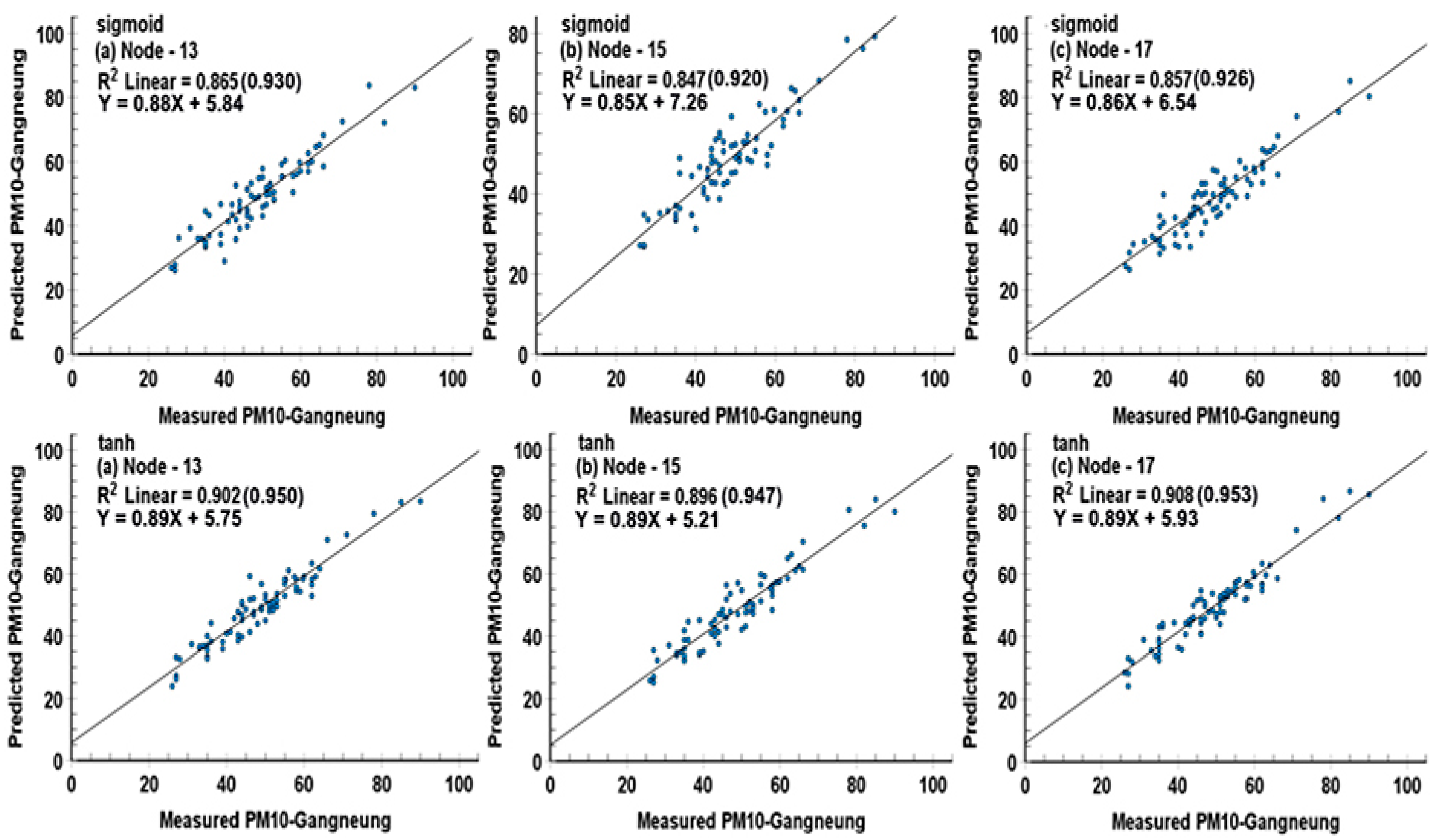
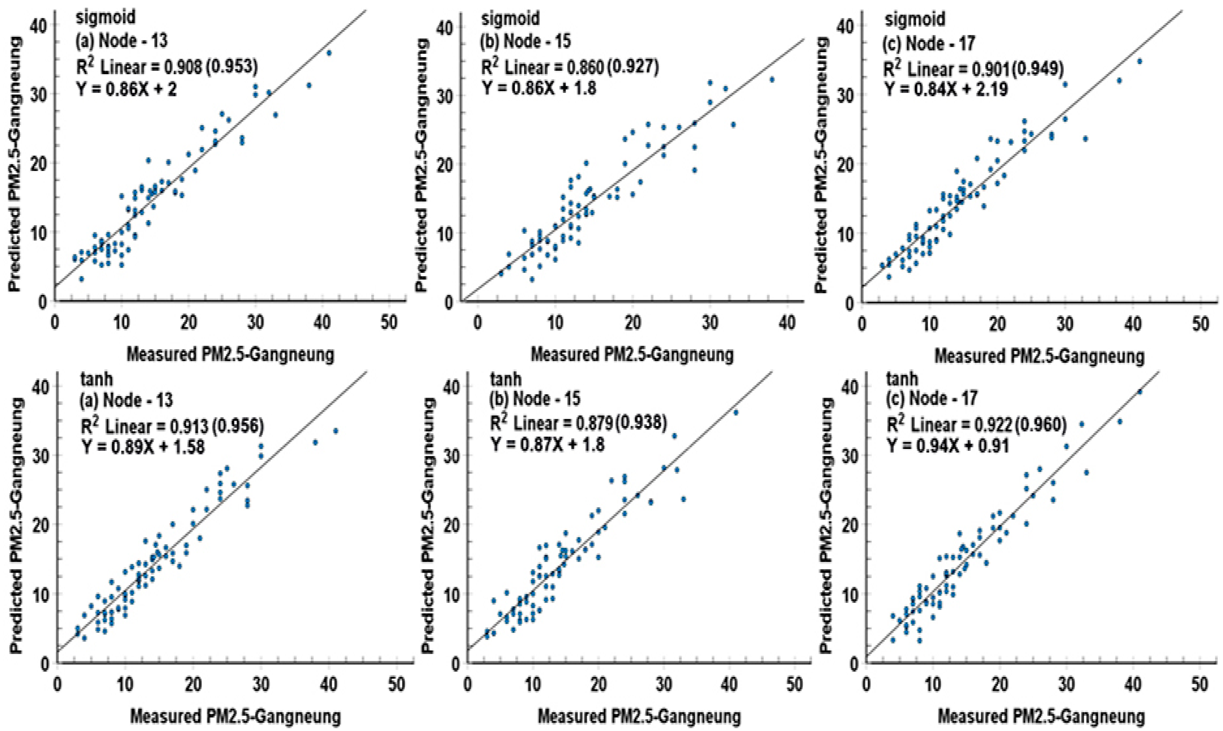
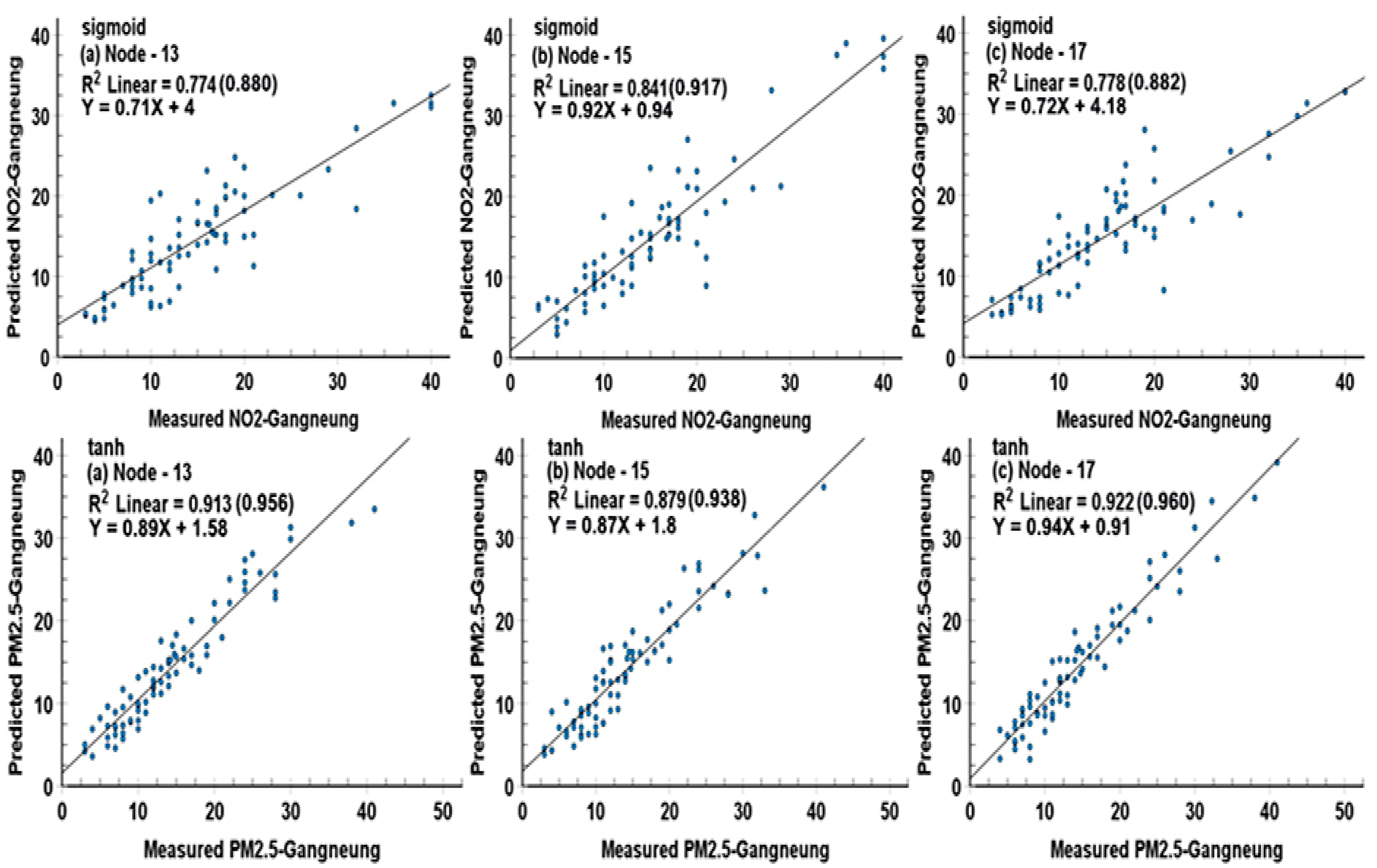
Using the only validation data for the two models’ simulation, scatter plots were depicted with empirical equations, and R² (or Pearson R) was evaluated from the relationship between the predicted and measured values to assess their prediction accuracy. Figure 3, Figure 4 and Figure 5 denote scatter plots with empirical equations and R² between the predicted and measured values of PM₁₀ (μg/m³), PM_2.5 (μg/m³), and NO₂ (ppm × 1000) concentrations, using the ANN-sigmoid and ANN−tanh models in Gangneung in March 2015.

Figure 3. Scatter plots with empirical equations and R² between the predicted and measured PM₁₀ (μg/m³) concentrations by ANN-sigmoid and ANN–tanh models in Gangneung city in March 2015.

Figure 4. As shown in Figure 3, except for and PM_2.5 (μg/m³).

Figure 5. As shown in Figure 3, except for NO₂ (ppm × 1000).

Since very high Pearson R values were in the range of 0.917 to 0.953 (ANN-sigmoid), and 0.938 to 0.960 (ANN-tanh) for PM₁₀ and PM_2.5, except for 0.880 (0.880) for NO₂ in sigmoid, and 0.886 in tanh, the two models maintain the excellent prediction performance for air quality, regardless of the activation functions and hidden node numbers. However, the ANN-tanh model showed clearly better prediction ability than the ANN-sigmoid model, and the more mode numbers in the hidden layer, the better the prediction model.

Generally, the ANN-tanh model with 17 hidden nodes produced the best prediction accuracy, but their discrepancy among the R values was very small. Users may decide for themselves the activation function and the hidden node numbers for an optimal forecasting model. In this study, the empirical formula derived from the correlation between the predicted and measured values suggested by the two models’ simulation can be well used to predict the air quality state at the forecasting time and sequentially at a certain future time interval.

4.2.2. Sensitivity of the ANN Model Prediction Performance

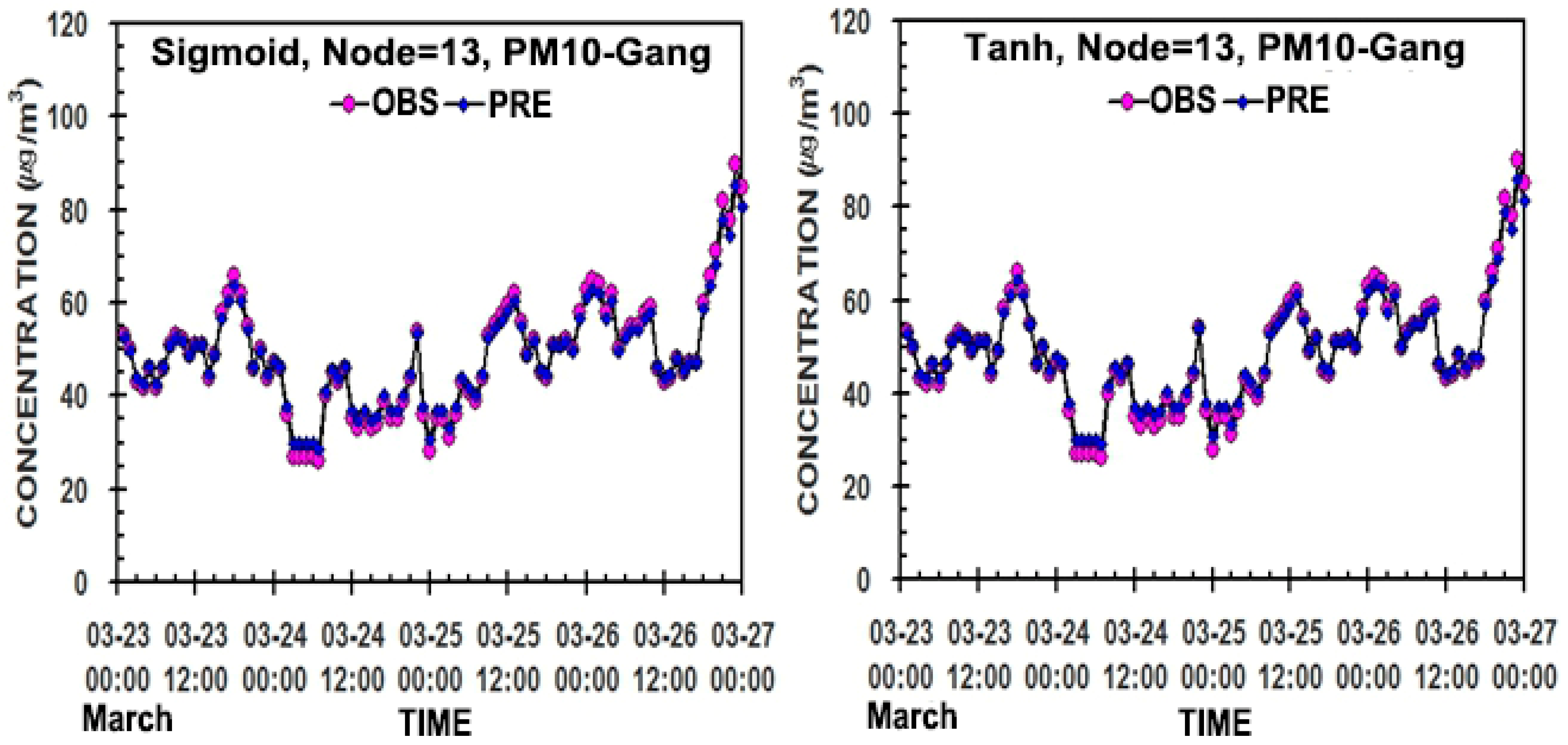
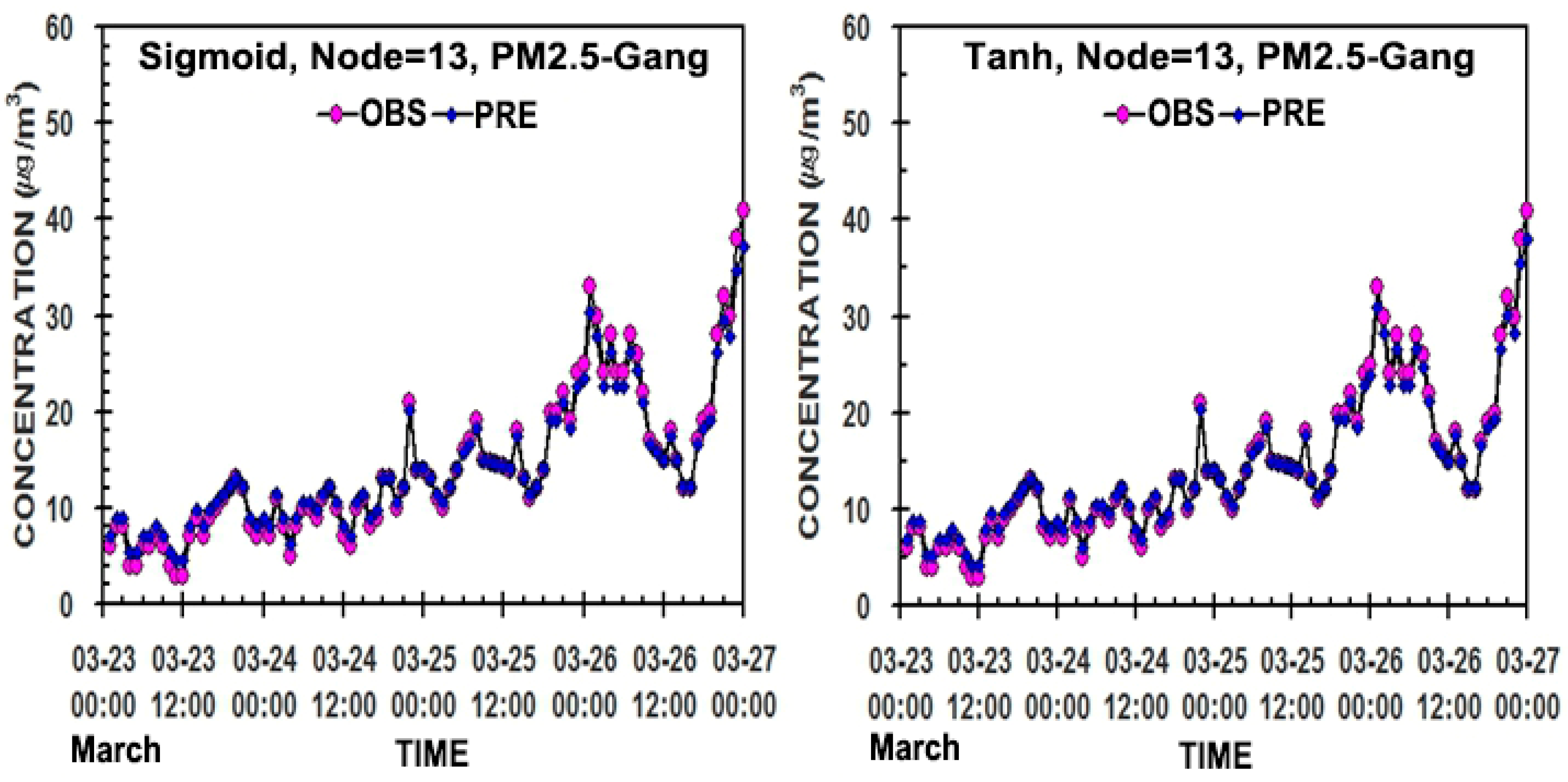
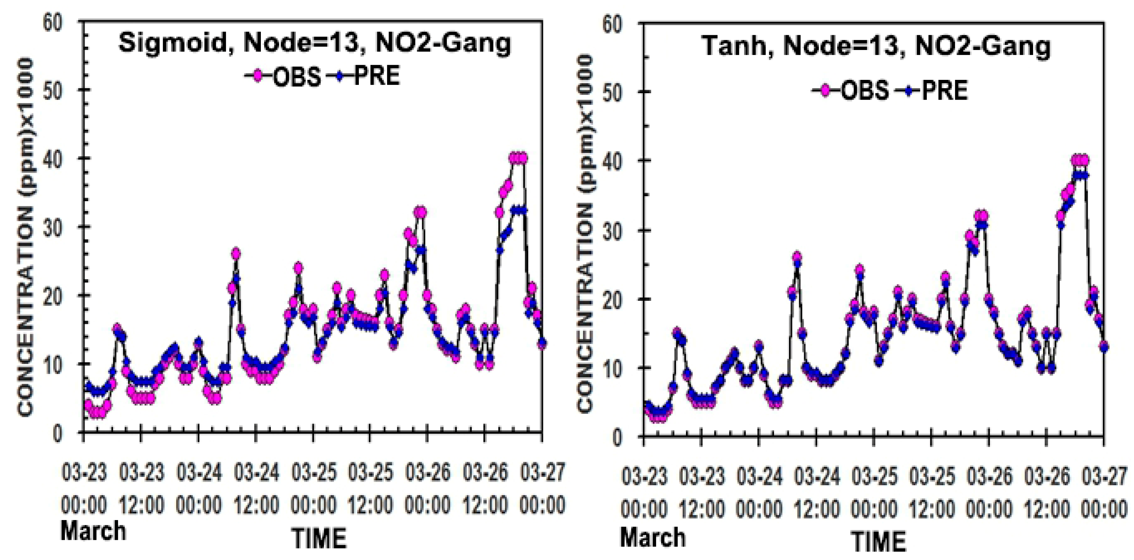
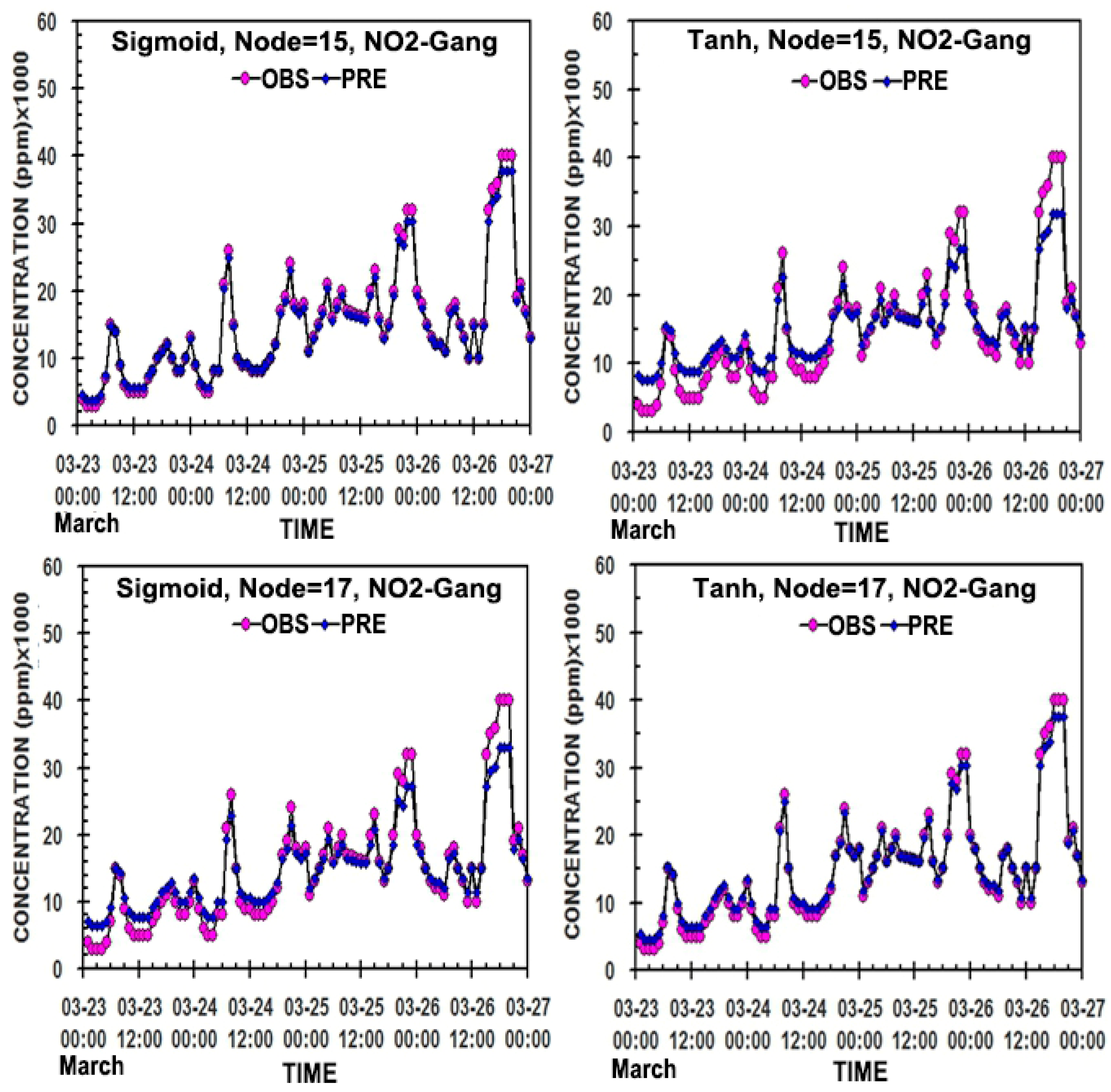
Figure 6, Figure 7 and Figure 8 present the hourly distributions of the predicted values of PM₁₀, PM_2.5, and NO₂ concentrations to compare with their measured values in 13, 15, and 17 nodes in the hidden layer of the two models. Regardless of different node numbers and activation functions, the predicted values of PM₁₀ and PM_2.5 through the two models’ simulations were very close to the measured ones, except for a slight bias in 13 and 17 nodes in sigmoid and 15 nodes in tanh for NO₂ (Table 2, Figure 3, Figure 4 and Figure 5).

Figure 6. Comparison of the predicted to measured hourly PM₁₀ (μg/m³) in the hidden neurons of 13, 15, and 17 in the two ANN models in Gangneung, Republic of Korea.

Figure 7. As shown in Figure 6, except for PM_2.5 (μg/m³) in the hidden neurons of 13, 15, and 17 in the two ANN models.

Figure 8. As shown in Figure 6, except for NO₁ (PPM × 1000) in the hidden neurons of 13, 15, and 17 in the two ANN models.

Thus, overall, except for the case of NO₂, the predicted values by the ANN-tanh model reflect the measured values much better than those by the ANN-sigmoid model, and so it can be used more effectively as an air quality prediction model. Namely, the more nodes in the hidden layer, the better the prediction results. However, the ANN-sigmoid model will also be useful because it still has an excellent prediction ability, due to a small difference in the prediction ability compared with the ANN-tanh model.

In this study, 15 input independent variables—3 hours’ earlier PMs (PM₁₀, PM_2.5), gaseous (NO₂, SO₂, CO, O₃) and meteorological data (air temperature, wind speed, relative humidity) of Gangneung city (Republic of Korea), and 2 days’ earlier PMs, gaseous of Beijing city (China) in the dust transport route—were designed to predict current urban air quality state of Gangneung city by utilizing artificial neural network (ANN-sigmoid and ANN-Tanh). In addition, using a similar model, the later air quality forecasting state at a certain future time can be calculated sequentially.

However, it is not easy to find research papers to explain how much the effect of different node numbers in the hidden layer of the ANN for air quality forecasting exists. Roy [36] explained that if the number of neurons in the hidden layer is set too small, the artificial neural network will underfit, and if it is set too large, it will overfit. It is important that the present study cannot agrees with his claim; if the number of neurons in the hidden layer is set too small (large), the artificial neural network will underfit (overfit). Because the current study revealed clearly that the prediction performance is slightly better when the number of neurons in the hidden layer than input layer is larger or smaller, as shown in Table 2, Figure 3, Figure 4, Figure 5, Figure 6, Figure 7 and Figure 8.

In addition, for showing the prediction accuracy of the current modeling works (the same (15 nodes) and different nodes (13, 17 nodes) in the hidden layer than the input layers) compared to the other research papers (with the same nodes in both input and hidden layers), Table 3 is given for the comparison of the Person r correlation coefficients between the predicted and measured values using the SVR, random forest, LSTM, ANN-sig, ANN-tanh, and multivariate regression models using hourly and daily averaged data. The maximum value of R by the ANN-sigmoid (ANN-tanh) model was 0.930 (0.953) on PM10, 0.953 (0.960) on PM_2.5, and 0.917 (0.959) on NO₂, and their prediction accuracies are very high, compared to the simulation results by other scientists.

Table 3. Comparison of the prediction accuracies on the various models performed by the authors for the non- and yellow dust (YD) with the Pearson R correlation coefficients. SVM, RF, ANN-sig, ANN-tanh, multivariate, and LSTM denote super vector machine, random forest, artificial neural network with sigmoid, artificial neural network with tanh, multivariate regression, and long short-term memory, respectively.

Pearson R
Author	Model	(Hourly) Before YD			(Hourly) During YD			(Hourly) After YD			(Hourly)-Non YD (Daily)
		PM10	PM2.5	NO2	PM10	PM2.5	NO2	PM10	PM2.5	NO2	PM10	PM2.5	NO2	PM10	PM2.5	NO2
Jeon and Son (2018) [33]	SVM													0.751
	RF													0.726
	ANN-sig													0.737
Kim (2019) [26]	Multivariate													0.849
Lee and Lee (2020) [34]	ANN-sig											0.837
	LSTM											0.907
	RF											0.910
Choi, et al. (2023) [17]	Multivariate	0.957	0.906	0.886	0.936	0.982	0.866	0.919	0.945	0.902
Choi (2024) [35]	ANN-tanh	0.935	0.942	0925	0.943	0.969	0.853	0.947	0.938	0886
	Multivariate	0.961	0.909	0.896	0.948	0.977	0.875	0.920	0.947	0.903
Choi (present)	ANN-sig										0.930	0.953	0.917
	ANN-tanh										0.953	0.960	0.959

5. Conclusions

The main purpose of this paper is focused to explain how much influence of different node numbers in the hidden layer (such as 13, 15, or 17 nodes) than input layer (15 nodes) of the artificial neural network model (ANN) and the different activation functions for air quality forecasting, even though each pollutant prediction of typical urban air pollutants of PM₁₀, PM_2.5, and NO₂ concentrations itself at the current and future times. Unfortunately, it is not easy to find research papers to explain how much the effect of different node numbers in the hidden layer of the ANN with different activation functions for air quality forecasting exists.

Thus, the air quality forecasting to explain how the node numbers (larger or smaller) in the hidden layer than the input layer of artificial neural network (ANN) models, associated with the different activation functions (sigmoid or hyperbolic tangent), were investigated in Gangneung city (Republic of Korea), and the results in this study are given below:

(1)

The two models’ forecasting abilities between the predicted and measured values show the values of Pearson R by ANN-sig (ANN-tanh) with different 13, 15, or 17 node numbers in the hidden layer than input layer (15 nodes) were 0.930 (0.950), 0.920 (0.947), and 0.926 (0.953) on PM10, 0.953 (0.956), 0.927 (0.938), and 0.949 (0.960) on PM2.5, and 0.880 (0.959), 0.917 (0.886), and 0.882 (0.939) on NO₂.

(2)

Regardless of different node numbers and activation functions, the predicted values of PM₁₀ and PM_2.5 through the two models’ simulations were very close to the measured ones, except for a slight bias of the predicted values in 13 and 17 hidden nodes with the sigmoid function and 15 nodes with the tanh function for NO₂.

(3)

Overall, the predicted values by the ANN-tanh model reflect the measured ones better than those by the ANN-sigmoid model, and so, it is recommended as an optimal prediction model. However, the ANN-sigmoid model will also be useful because it still has an excellent prediction ability, due to a small discrepancy in the prediction ability as compared with the ANN-tanh model.

(4)

More nodes (17 nodes) in its hidden layer than the input layer (15 nodes) produce better prediction results in the two models, as shown in their temporal distributions and scatter plots. Thus, the current study cannot agree with Roy’s instance, such as underfitting in small node numbers in the hidden layer, overfitting in larger node numbers, and bestfitting in the same node numbers in the input layer.

(5)

Another importance is that the suggested two models can be used effectively to predict the current urban air quality state of Gangneung city (Republic of Korea), using previous time input variables (air pollutants-PM₁₀, PM_2.5, SO₂, NO₂, CO, and O₃; meteorological elements—air temperature, wind speed, and relative humidity) affected by the 48 hours earlier air pollutants of the upwind Beijing city (China).

(6)

In a similar way, later air quality forecasting state of Gangneung city at a certain future time (such as 3 h later) can be calculated sequentially, using the current urban air quality and meteorological data sets (Gangneung city), and the 45 hours earlier pollutant data (Beijing city). Practically, the empirical formula derived from the correlation between the predicted and measured values suggested through the two models’ simulation can be well used to predict the air quality state, at the forecasting time, and sequentially at a certain future time.

Future studies will further improve air quality prediction ability using various artificial neural network activation functions, compared with the results of numerical prediction models on air pollution dispersion.

References

1. Lee, S.C.; Cheng, Y.; Ho, K.F.; Cao, J.J.; Loui, P.K.K.; Chow, J.C.; Watson, J.G. PM10 and PM2.5 characteristics in the roadside environment of Hong Kong. Aerosol. Sci. Tech. 2006, 40, 157–165. [Google Scholar] [CrossRef]
2. Park, D.; Ha, K. Characteristics of PM10, PM2.5, CO2 and CO monitored in interiors and platforms of subway train in Seoul, Korea. Environ. Int. 2008, 34, 629–634. [Google Scholar] [CrossRef]
3. Hamilton, R.; Kucera, V.; Tidblad, J.; Watt, J. The Effect of Air Pollution on Cultural Heritage; Springer: New York, NY, USA, 2012; pp. 1–306. ISBN 978-0-387-84892-1. [Google Scholar] [CrossRef]
4. Huang, D.; Xu, J.; Zhang, S. Valuing the health risks of particulate air pollution in the Pearl River Delta, China. Environ. Sci. Policy 2012, 15, 38–47. [Google Scholar] [CrossRef]
5. Li, F.; Liu, Y.; Lu, J.J.; Hamer, P. Ambient air pollution in China poses a multi-faceted health threat to outdoor physical activity. J. Epidem. Comm. Health 2015, 69, 201–204. [Google Scholar] [CrossRef] [PubMed]
6. He, J.Q.; Yu, X.N.; Zhu, B.; Yuan, L.; Ma, J.; Shen, L.; Zhu, J. Characteristics of Aerosol Extinction and Low Visibility in Haze Weather in Winter of Nanjing, China. Environ. Sci. 2016, 36, 1645–1653. [Google Scholar]
7. Li, C.; Dai, Z.; Yang, L.; Ma, Z. Spatiotemporal characteristics of air quality across Weifang from 2014–2018. Int. J. Environ. Res. Pub. Health 2019, 16, 3122. [Google Scholar] [CrossRef]
8. Zhang, X.; Han, L.; Wei, H.; Tan, X.; Zhou, W.; Li, W.; Qian, Y. Linking urbanization and air quality together: A review and a persective on the future sustainable urban development. J. Clear Prod. 2022, 346, 130988. [Google Scholar] [CrossRef]
9. Gul, H.; Das, B.K. The Impacts of Air Pollution on Human Health and Well-Being: A Comprehensive Review. J. Environ. Impact Manag. Policy 2023, 36, 11. [Google Scholar] [CrossRef]
10. Zhang, X.; Arimoto, R. Atmospheric trace elements over source regions for Chinese dust: Concentrations, sources and atmospheric deposition on the losses plateau. Atmos. Environ. 1993, 27, 2051–2067. [Google Scholar] [CrossRef]
11. Chon, H. Historical records of yellow sand observations in China. Res. Environ. Sci. 1994, 7, 1–11. [Google Scholar]
12. Carmichael, G.R.; Hong, M.S.; Ueda, H.; Chen, L.L.; Murano, K.; Park, J.K.; Lee, H.; Kim, Y.; Kang, C.; Shim, S. Aerosol composition at Cheju Island, Korea. J. Geophys. Res. 1997, 102, 6047–6061. [Google Scholar] [CrossRef]
13. Chung, Y.S.; Yoon, M.B. On the occurrence of yellow sand and atmospheric loadings. Atmos. Environ. 1996, 30, 2387–2397. [Google Scholar] [CrossRef]
14. Wang, X.; Ma, Y.; Chen, H.; Wen, G.; Chen, S.; Tao, Z.; Chung, Y. The relation between sandstorms and strong winds in Xinjiang, China. Water Air Soil Poll. Focuss 2003, 3, 67–79. [Google Scholar] [CrossRef]
15. Choi, H.; Zhang, Y.H. Predicting duststorm evolution with vorticity theory. Atmos. Res. 2008, 89, 338–350. [Google Scholar] [CrossRef]
16. Choi, H.; Choi, D.S.; Choi, S.-M. Meteorological condition and atmospheric boundary layer influenced upon temporal concentrations of PM1, PM2.5 at a Coastal City, Korea for Yellow Sand Event from Gobi Desert. Disaster Adv. 2010, 3, 309–315. [Google Scholar]
17. Choi, S.-M.; Choi, H.; Paik, W. Multivariate regression modeliing for coastal urban air quality estimate. Appl. Sci. 2023, 12, 1638. [Google Scholar] [CrossRef]
18. Kotamarthi, V.R.; Carmichael, G.R. The long range transport of pollutants in the Pacific Rim region. Atmos. Environ.-A 1990, 24, 1521–1534. [Google Scholar] [CrossRef]
19. David, M.T.; Robert, J.F.; Douglas, L.W. April 1998 Asian dust event: A southern California perspective. J. Geophys. Res. 2001, 106, 18371–18379. [Google Scholar] [CrossRef]
20. Lin, T.H. Long-range transport of yellow sand to Taiwan in spring 2000: Observed evidence and simulation. Atmos. Environ. 2001, 35, 5873–5882. [Google Scholar] [CrossRef]
21. McKendry, I.G.; Hacker, J.P.; Stull, R.; Sakiyama, S.; Mignacca, D.; Reid, K. Long-range transport of Asian dust to the lower Fraser Valley, British Columbia, Canada. J. Geophys. Res. 2001, 106, 18361–18370. [Google Scholar] [CrossRef]
22. Uno, I.; Amano, H.; Emori, S.; Kinoshita, K.; Matsui, I.; Sugimoto, N. Tans-Pacific yellow sand transport observed in April, 1998: A numerical simulation. J. Geophys. Res. 2001, 106, 18331–18344. [Google Scholar] [CrossRef]
23. Jeong, U.; Kim, J.; Lee, H.; Lee, Y.G. Assessing the effect of long-range pollutant transportion on air quality in Seoul using the conditional potential source contribution function method. Atmos. Environ. 2017, 150, 33–44. [Google Scholar] [CrossRef]
24. Kong, S.S.; Babu, S.R.; Wang, S.-H.; Griffith, S.M.; Chang, J.H.-W.; Chung, M.-T.; Sheu, G.-R.; Lin, N.-H. Expanding the simulation of east Asian super dust storms: Physical transport mechanisms impacting the western Pacific. Atmos. Chem. 2024, 24, 1041–1058. [Google Scholar] [CrossRef]
25. Li, X.; Ma, Y.; Wang, Y.; Liu, N.; Hong, Y. Temporal and spatial analyses of particulate matter (PM10 and PM2.5) and its relationship with meteorological parameters over an urban city in northeast China. Atmos. Res. 2017, 198, 185–193. [Google Scholar] [CrossRef]
26. Kim, M.J. The effects of transboundary air pollution from China on ambient air quality in South Korea. Heliyon 2019, 5, e02953. [Google Scholar] [CrossRef]
27. Choi, S.-M.; Choi, H. Statistical modeling for PM10, PM2.5, and PM1 at Gangneung affected by local meteorological variables and PM10 and PM2.5 at Beijing for non- and dust periods. App. Sci. 2021, 11, 11958. [Google Scholar] [CrossRef]
28. Masters, T. Practical Neural Network Recipes in C++; Academic Press: San Diego, CA, USA, 1993. [Google Scholar]
29. Shahin, M.A.; Jaksa, M.B.; Maier, H.R. Artificial neural network based settlement prediction formula for shallow foundations on granular soils. Aust. Geomech. J. 2002, 36, 49–62. [Google Scholar]
30. Gao, S.; Liu, Y.; Zhang, J.; Yu, J.; Chen, L.; Sun, Y.; Mao, J.; Zhang, H.; Ma, Z.; Yang, W.; et al. Soil-derived dust PM10 and PM2.5 fractions in Southern Xinjiang, China, using an artificial neural network model. Atmosphere 2023, 14, 1644. [Google Scholar] [CrossRef]
31. Nawras, S.; Hani, A.-Q. Assessing and predicting air quality in northern Jordan during the lockdown due to the COVID-19 virus pandemic using artificial neural network. Air. Qual. Atmos. Health 2021, 14, 643–652. [Google Scholar] [CrossRef]
32. Choi, S.-M.; Choi, H. Artificial neural network modeling on PM10, PM2.5 and NO2 concentrations between two megacities without a lockdown in Korea, for the COVID-19 pandemic period of 2022. Int. J. Environ. Res. Public Health 2022, 19, 16338. [Google Scholar] [CrossRef]
33. Jeon, S.; Son, Y.S. Prediction of fine dust PM10 using a deep neural network model. Korean J. Appl. Stat. 2018, 31, 205–285. [Google Scholar] [CrossRef]
34. Lee, D.; Lee, S. Hourly prediction of particulate matter (PM2.5) concentration using time series data and random forest. KIPS Trans. Softw. Data Eng. 2020, 9, 129–136. [Google Scholar] [CrossRef]
35. Choi, S.-M. Improved air quality forecasting based on machine learning and multivariate regression techniques. Informatica 2024, 35, 2–19. [Google Scholar] [CrossRef]
36. Roy, D.S. Forecasting the air temperature at a weather station using deep neural networks. Procedia Comput. Sci. 2020, 178, 38–46. [Google Scholar] [CrossRef]
37. Rumelhart, D.E.; Hinton, G.E.; Williams, R. Learning representations by back-propagation error. Nature 1996, 323, 533–536. [Google Scholar] [CrossRef]
38. Dhakal, S.; Gautam, Y.; Bhattaral, A. Evaluation of temperature based empirical model and machine learning technique to estimate daily global solar radiation at Biratnagar airport, Nepal. Adv. Meteorol. 2020, 11, 8895311. [Google Scholar] [CrossRef]
39. Jaiwal, S. Multilayer Percetrons in Machine Learning: A Comprehensive Guide. Available online: https://www.datacamp.com/tutorial/multilayer-perceptrons-in-machine-learning (accessed on 29 July 2024).
Disclaimer/Publisher’s Note: The statements, opinions and data contained in all publications are solely those of the individual author(s) and contributor(s) and not of MDPI and/or the editor(s). MDPI and/or the editor(s) disclaim responsibility for any injury to people or property resulting from any ideas, methods, instructions or products referred to in the content.
Article Metrics
Citations
Article Access Statistics
Article metric data becomes available approximately 24 hours after publication online.