Abstract
Deterministic chaos in optically injected semiconductor lasers (OILs) has attracted significant attention due to its relevance in secure communications, entropy generation, and photonic applications. However, existing studies often rely on low-resolution parameter sweeps or include noise contributions that obscure the intrinsic nonlinear dynamics. To address this gap, we investigate a noise-free OIL model and construct high-resolution chaos maps across the injection strength and frequency detuning parameter space. Chaos is characterized using two complementary approaches for computing the largest Lyapunov exponent: the Rosenstein time-series method and the exact variational method. This dual approach provides reliable and reproducible detection of deterministic chaotic regimes and reveals a rich attractor landscape with alternating bands of periodicity, quasi-periodicity, and chaos. The novelty of this work lies in combining high-resolution mapping with rigorous chaos indicators, enabling fine-grained identification of dynamical transitions. The results not only deepen the fundamental understanding of nonlinear laser dynamics but also provide actionable guidelines for exploiting or avoiding chaos in photonic devices, with potential applications in random chaos-based communications, number generation, and optical security systems.
1. Introduction
Chaotic signal generation using optically injected laser (OIL) systems has emerged as a powerful technique within the field of nonlinear photonics, offering a compact, tunable, and high-speed platform for exploiting the complex dynamics of semiconductor lasers [1]. When a slave laser receives coherent light from a master laser under specific conditions—such as frequency detuning and injection strength—the coupled system can transition into a chaotic regime [2]. This regime is characterized by deterministic yet unpredictable behavior and broadband spectral features.
Chaotic systems are characterized by deterministic nonlinear dynamics that exhibit extreme sensitivity to initial conditions, broadband spectra, and a mixture of order and unpredictability. Their construction typically arises from simple equations with nonlinear feedback, yet they generate complex trajectories useful in multiple applications. Beyond fundamental studies, chaos has been widely exploited in secure communications, random number generation, sensing, and encryption technologies. In particular, chaos-based encryption schemes take advantage of the unpredictability and sensitivity of chaotic signals to design cryptographic protocols that are resistant to brute-force and differential attacks, while maintaining low computational cost. Recent advances in related fields illustrate the continuing vitality of chaos research: memristive neural networks have been shown to display rich chaotic dynamics with practical implications for hardware implementation and information security [3,4]; fractional-order Hopfield networks combined with differentiated encryption have been proposed for high-performance privacy protection in medical images [5]; and novel logistic modular maps with enhanced vector-level operations have been designed for efficient chaotic image encryption [6].
In recent years, the ability to harness this optical chaos has opened new frontiers in various technological domains. One prominent application is in secure optical communications [7,8], where chaotic waveforms are used to mask information, enhancing resistance to eavesdropping and improving data encryption. Similarly, true random number generation, essential for cryptographic protocols, benefits from the inherent unpredictability of chaotic laser signals, delivering high-speed and high-entropy outputs. Another growing area is microwave photonics, where chaotic carriers enable ultra-wideband signal processing and waveform generation [9]. Moreover, chaotic lasers have shown promise in neuromorphic computing, mimicking the complex spiking dynamics of biological neurons for use in artificial neural networks [10]. They are also being explored in sensor systems for enhancing sensitivity and in reservoir computing paradigms that use chaotic dynamics for efficient temporal information processing. As integrated photonics continues to evolve, the miniaturization and on-chip integration of chaotic laser sources are becoming increasingly feasible [11]. This advancement enables the development of compact and energy-efficient platforms for secure data transmission [12], AI acceleration, and quantum technologies [2].
Another key application of chaotic dynamics is in random number generation (RNG), where the unpredictability and broadband nature of chaotic signals are harnessed to produce entropy sources with high statistical quality. Recent advances illustrate the diversity of photonic platforms enabling chaos-based RNG. For instance, self-chaotic microlasers with enhanced chaotic bandwidth have been demonstrated as efficient random bit generators [13], while integrated silicon photonics has been exploited to realize compact quantum random number generators using laser diodes [14]. At a larger scale, microcomb-based chaos provides massive parallel random bit generation [15], and long-haul chaos synchronization experiments highlight the potential of secure RNG over optical links [1]. Efforts have also been made to stabilize chaos and prevent intermittency in RNG-oriented semiconductor lasers [16]. These developments confirm the importance of chaos as a robust and scalable entropy source, reinforcing its role in secure communications and photonic information processing.
In recent years, chaos-based optical communication has rapidly advanced from proof-of-concept demonstrations to high-capacity and long-haul secure transmission systems. Spitz et al. demonstrated private communication using quantum cascade laser photonic chaos, highlighting the potential of chaotic semiconductor sources for physical-layer security [17]. Building on this foundation, Xie et al. achieved 100 Gb/s coherent chaotic optical communication over 800 km fiber transmission with advanced digital signal processing [18], while Wang et al. demonstrated high-speed secure communications over a 130 km multi-core fiber using mutual injection of semiconductor lasers and space-division multiplexing techniques [19]. Feng et al. further realized 256 Gb/s chaotic optical communication over 1600 km by combining chaos synchronization with an AI-driven optoelectronic oscillator model, marking a leap in both speed and distance [20]. Mao et al. reported 100 Gb/s secure fiber-optic communication over 100 km using wideband chaotic semiconductor lasers with Nyquist half-cycle subcarrier modulation [21], and Wang et al. pushed the distance limit even further, experimentally demonstrating chaos synchronization over 8190 km of fiber, paving the way for submarine and backbone network applications [1]. Taken together, these works illustrate the rapid evolution of chaos-based optical communications toward practical, high-speed, and ultra-long-distance secure transmission systems.
The present study complements these advances by providing high-resolution chaos maps of OILs, offering a deterministic and reproducible framework to identify operating regions that yield broadband chaos versus stable periodic behavior. While recent experimental demonstrations have successfully transmitted encrypted data streams over distances ranging from hundreds to thousands of kilometers [1,13,17,18,19,20,21], the precise parameter ranges that favor robust chaos generation remain difficult to delineate experimentally due to the interplay of detuning, injection strength, and noise. Our maps directly address this gap: by linking dynamical indicators such as the largest Lyapunov exponent (LLE) and dissipativity to specific injection–detuning pairs, we provide actionable design guidelines for configuring OIL-based transmitters in chaos-secure communication systems. In this way, the deterministic mapping developed here serves as a theoretical foundation that enhances and informs ongoing experimental efforts toward scalable, high-capacity, and ultra-long-haul chaos-based optical communication.
Together, these developments demonstrate the broad relevance of chaos studies across disciplines. By extending chaos applications from electronic neural networks to photonic devices, such as optically injected semiconductor lasers (OILs), the field gains access to ultrafast chaotic carriers suitable for high-speed optical encryption, real-time secure communication, and photonic random number generation. This reinforces the importance of exploring OILs as a versatile and experimentally accessible platform for deterministic chaos, bridging fundamental nonlinear science with applied information security.
Previous experimental work has demonstrated the existence of periodic and aperiodic pulsing regimes in OILs, highlighting their dependence on injection parameters such as power ratio and frequency detuning [22]. Subsequent numerical studies developed automated methods to detect such regimes and mapped their presence near the static synchronization boundary, based on signal metrics such as extrema count and total harmonic distortion [23]. However, the exact boundaries where chaotic dynamics emerge—particularly those associated with geometric and homoclinic chaos—remain poorly resolved. Furthermore, recent simulations incorporating stochastic noise have shown that aperiodic and potentially chaotic behavior can arise due to noise–laser interactions, emphasizing the role of intrinsic perturbations in destabilizing pulsing regimes [24]. In this work, we systematically identify the regions of optical injection parameters that give rise to chaos, combining time-domain simulations with chaos indicators to produce high-resolution maps of chaotic behavior in the injection strength and frequency detuning space. Our results contribute to a more comprehensive understanding of nonlinear laser dynamics and enable improved control strategies for applications requiring or avoiding chaotic outputs.
In this paper, we compute the maximum Lyapunov exponent of the OIL system using two distinct approaches. The first is an approximate method based on the algorithm proposed by Rosenstein et al. [25], which estimates the exponent directly from time-series data by reconstructing the system’s attractor in a delay-coordinate embedding space. While this method is widely used due to its simplicity and applicability to experimental data, it relies on the choice of embedding parameters and can be sensitive to noise and finite data length. To complement this, we also apply a more rigorous technique: the variational method. This approach involves the simultaneous integration of the nonlinear system equations and their associated variational (Jacobian) equations. By tracking the evolution of perturbation vectors in tangent space and periodically orthonormalizing them (e.g., via QR decomposition), the method provides a precise and dynamic estimate of the full Lyapunov spectrum. Unlike the approximate method, the variational approach is deterministic, does not require embedding, and yields high-resolution insight into the system’s local stability properties. Its rigor and accuracy make it especially valuable for the theoretical analysis of continuous dynamical systems such as the OIL model studied here.
Characterizing chaotic regimes in OILs is essential for applications in secure communications, random number generation, and neuromorphic photonics [26]. However, the presence of stochastic contributions, such as spontaneous emission noise and Langevin forces, complicates the analysis of underlying deterministic dynamics. These noise sources can obscure or mimic chaos, leading to false-positive indicators in commonly used metrics such as the Lyapunov exponent or power spectral density. To overcome this limitation, we perform a chaos analysis on noise-free OIL models in which the nonlinear dynamics are isolated from quantum and thermal fluctuations. This approach ensures that any observed complexity originates from deterministic mechanisms inherent to the injection dynamics, and provides a reproducible and reliable baseline for later evaluating the robustness of chaos in realistic noisy conditions.
The main contributions of this work can be summarized as follows:
- We develop high-resolution maps of chaos in OILs, resolving fine bifurcation structures across injection strength and frequency detuning.
- We apply and compare two complementary methods for chaos detection: the Rosenstein algorithm on time-series data and the exact variational method, demonstrating their agreement and complementarity.
- We introduce a methodological framework that is reliable, reproducible, and extendable to other classes of semiconductor lasers.
- We link the numerical chaos maps to potential applications in secure communications, random number generation, and photonic systems.
The remainder of the paper is organized as follows: Section 2 presents the theoretical model, numerical methodology, and Lyapunov analysis tools. Section 3 describes the construction of high-resolution chaos maps and provides detailed interpretations of the results. Section 4 discusses the implications of the maps in relation to prior studies and applications. Section 5 concludes the work by summarizing the contributions and outlining directions for future research.
2. Method
OILs offer a compact and cost-effective platform for generating complex optical signals, without requiring external modulators or RF electronics. By carefully tuning the injection parameters—specifically, the power injection ratio and frequency detuning between the master laser (ML) and the slave laser (SL)—OILs can exhibit a broad spectrum of nonlinear dynamics. These include chaotic signals, quasi-periodic waveforms, and quasi-periodic pulse trains, making OILs highly versatile for applications such as secure communications, random number generation, and neuromorphic computing [27,28].
OILs are often modeled using the Kobayashi–Lang equations, which form a system of three coupled nonlinear differential equations [27,28]. The first equation governs the amplitude of the slave laser (SL) field, denoted as . The second describes the phase difference between the SL and the master laser (ML), defined as . The third models the carrier density within the SL gain region. When including stochastic noise terms, the system can be written as
Here, g is the linear gain coefficient, is the injected ML field amplitude, and is the linewidth enhancement factor. The coupling coefficient accounts for the injection strength and depends on the mirror reflectivity r, the injection efficiency , and the round-trip time , given by
The detuning frequency is defined as . The term J denotes the carrier injection rate, while and are the photon decay rate and carrier recombination rate, respectively. The functions R, and represent Spontaneus and Langevin noise contributions associated with field amplitude and phase fluctuations.
To rigorously characterize deterministic chaos in OILs, it is critical to remove spontaneous emission and Langevin noise, which obscure the system’s intrinsic nonlinear dynamics and can mimic chaotic signatures [26,29]. These stochastic perturbations compromise reproducibility, distort phase space structures, and undermine key chaos indicators such as Lyapunov exponents, correlation dimension, and spectral features [30,31]. In noisy conditions, trajectories diverge inconsistently, strange attractors become ill-defined, and autocorrelation functions resemble white noise, making chaos indistinguishable from stochastic fluctuations. By suppressing noise, the system’s complexity can be unambiguously attributed to deterministic feedback mechanisms like phase detuning and carrier–photon interactions.
2.1. Physical Mechanisms Underlying the Simulations
The optically injected laser dynamics arise from the balance between (i) carrier-induced gain that amplifies the optical field amplitude , (ii) cavity and material losses that dissipate photons and carriers, and (iii) coherent forcing from the master laser characterized by injection strength (power ratio in dB) and frequency detuning . The linewidth enhancement factor couples carrier-induced refractive index changes to phase dynamics, enabling amplitude–phase feedback that underlies bifurcations. Increasing the injection ratio and tuning detuning can drive the system from locked or periodic operation into quasi-periodicity and chaos via torus breakdown or homoclinic mechanisms. In the variational framework, the trace of the Jacobian gives the instantaneous phase space divergence, and the long-time average equals the sum of Lyapunov exponents, which diagnoses dissipativity and the effective contraction toward low-dimensional attractors.
To capture these mechanisms under experimentally realistic conditions, numerical simulations of the OIL system were carried out using the parameter set listed in Table 1. These values are based on typical semiconductor laser characteristics reported in the literature [22,32], and include the ranges of injection strength and frequency detuning explored in the chaos maps.

Table 1.
Simulation parameters of the OIL system, including control parameter ranges, based on [22,32].
As we will see in the following subsections, the Rosenstein method was chosen for its practicality and computational efficiency, since it estimates the LLE directly from simulated time-series data of the laser amplitude . This makes it particularly suitable for extensive parameter sweeps. In contrast, the variational method provides a rigorous, model-based benchmark: by integrating the tangent dynamics of the Kobayashi–Lang equations, it yields the full Lyapunov spectrum . Using both approaches in tandem offers a balance between numerical efficiency and theoretical rigor, and their close agreement across the explored parameter space strengthens confidence in the reliability of the resulting chaos maps.
2.2. Approximate Estimation of the LLE
To detect the presence of deterministic chaos in the time-domain signals and characterize the sensitivity to initial conditions, we estimated the LLE using a MATLAB-2024 based implementation adapted from the Predictive Maintenance Toolbox. This method follows the approach described by Rosenstein et al. [25], which is robust for relatively short and noisy time series.
Given a uniformly sampled scalar signal , the algorithm reconstructs the underlying attractor dynamics via time-delay embedding, as per Takens’ theorem [33]. Each reconstructed state vector in D-dimensional phase space is defined as
where is the time delay (estimated from the first zero-crossing or point of the autocorrelation function) and D is the embedding dimension (often estimated via false nearest neighbors [34]).
For each state vector , the nearest neighbor is identified under the constraint , where ensures temporal separation and avoids autocorrelation bias. The divergence of nearby trajectories is tracked for s discrete time steps using
The average divergence is computed across all pairs and converted to a log-divergence curve:
The LLE is then estimated by performing a linear regression over the range of s where the divergence growth is approximately exponential:
The sign of the Lyapunov exponent determines the system behavior:
- : convergence of nearby trajectories (stable dynamics);
- : constant divergence (periodic or quasi-periodic);
- : exponential divergence (chaotic dynamics).
In our implementation, the time-delay embedding was performed using MATLAB’s phaseSpaceReconstruction function, and the exponent was extracted using a custom version of lyapunovExponent.m. The function also outputs diagnostic plots, including the log-divergence curve. This visualization helps verify the quality of the embedding and the validity of the exponential growth region used in the regression.
For each parameter pair , we first solve the Kobayashi–Lang rate equations, without stochastic noise terms, with a fourth–order Runge–Kutta (RK4) scheme using time step to obtain the amplitude time series . We then call lyapunovExponent where is the sampling frequency. The routine reconstructs the attractor (delay (L) and dimension (D), excludes temporal neighbors via a Theiler window (MinSeparation), computes the mean logarithmic divergence over expansion steps, and fits its linear region (ExpansionRange) to obtain LLE ().
This method provides an efficient approximation of the dominant Lyapunov exponent using a single trajectory. However, it yields only a partial view of the system’s full stability characteristics. In particular, it does not account for the full Lyapunov spectrum, nor can it distinguish between hyperchaotic and merely chaotic behavior. Therefore, for a more complete characterization of the system’s dynamics, especially in high-dimensional or multiscale systems, the computation of the exact Lyapunov exponents—typically via variational methods—is required.
2.3. Variational Method for Lyapunov Exponent Spectrum
To compute the full Lyapunov spectrum of the optically injected laser (OIL) system, we employ the variational method, a rigorous approach that integrates both the system’s nonlinear trajectory and its linearized tangent space dynamics [35,36]. This method is well suited for deterministic systems defined by differential equations and yields accurate, time-resolved estimates of all Lyapunov exponents.
2.3.1. Governing Equations
Let the state vector be , and let denote the nonlinear system of ODEs. The time evolution of the system is governed by
Simultaneously, the evolution of infinitesimal perturbations is governed by the linearized system
where is the Jacobian matrix evaluated along the trajectory, and is a matrix whose columns are tangent vectors initialized as an identity matrix.
2.3.2. Analytical Jacobian of the OIL Rate Equations
For the optically injected laser system defined by the state vector , the governing rate equations without stochastic noise terms are
The analytical Jacobian matrix is given by
This Jacobian is evaluated at each integration step and is critical for accurately computing the evolution of perturbation vectors in the tangent space. Its explicit form allows for efficient and precise implementation of the RK4 variational method, avoiding numerical approximations of partial derivatives.
2.3.3. Fourth-Order RK Integration of Base and Tangent Dynamics
Both the base system and the variational dynamics are integrated using the classical fourth-order Runge–Kutta (RK4) scheme. This approach ensures numerical consistency and stability across both trajectories.
System RK4 Integration
Let denote the system state at time , and the time step. The standard RK4 update is
Tangent Space RK4 Integration
Let be the tangent space matrix at step n. Using the Jacobian evaluated at the RK4 substeps of , we integrate the variational equation:
2.3.4. QR Decomposition and Lyapunov Exponents
To prevent numerical divergence and maintain orthonormality of tangent vectors, a QR decomposition is applied to at each step:
The Lyapunov exponents are accumulated as
where is the i-th diagonal entry of , N is the total number of steps, and is the integration time.
2.3.5. Advantages of the Variational Method
The variational method provides deterministic, high-resolution estimation of Lyapunov exponents, unaffected by noise or embedding parameters. Unlike approximate time-series methods such as those proposed by Rosenstein et al. [25], the variational approach directly leverages the system’s equations and their derivatives, yielding accurate results across the entire spectrum. Its ability to resolve local and global stability properties makes it particularly suitable for systems like the OIL, where precision and sensitivity to dynamical regimes are crucial.
2.4. Kaplan–Yorke Dimension
The Kaplan–Yorke (KY) dimension, also known as the Lyapunov dimension, provides a quantitative estimate of the fractal dimension of an attractor based on the Lyapunov spectrum [37]. Unlike the topological dimension, the KY dimension captures the effective number of degrees of freedom involved in the system’s chaotic behavior.
Given the ordered Lyapunov exponents , the Kaplan–Yorke dimension is defined as
where j is the largest integer such that . For three-dimensional systems such as the OIL model, this typically results in a dimension between 2 and 3 in the chaotic regime.
This dimension serves as a fractal complexity measure, estimating the number of active variables needed to describe the system’s long-term behavior. It also provides a useful tool to complement the maximum Lyapunov exponent, allowing us to distinguish between low- and high-dimensional chaotic attractors. In this work, the Kaplan–Yorke dimension was computed across the parameter space to generate a topological map of attractor complexity.
2.5. Dissipativity and Phase Space Volume Contraction
The sum of the Lyapunov exponents provides insight into the system’s global stability and phase space behavior. Specifically, it indicates whether the system is volume-preserving or dissipative:
For the OIL system, where , a negative sum implies that the system is dissipative, meaning that volumes in phase space contract over time. This contraction leads to the confinement of trajectories on lower-dimensional attractors, such as limit cycles or chaotic sets.
Dissipativity is a hallmark of nonlinear laser systems and is closely linked to the emergence of chaos. A strongly negative divergence generally corresponds to more compressed and stable attractors, while values approaching zero can indicate marginally stable dynamics or transitions to instability.
In this study, the total Lyapunov sum was computed alongside the spectrum to assess the dissipative nature of each operating point. This analysis confirms that chaotic regimes in the OIL system are associated with moderate dissipation, allowing for complex yet bounded dynamics within the phase space.
3. Results
We computed the maximum Lyapunov exponent using the two complementary methods described above. The first approach applies the Rosenstein algorithm, which estimates the LLE directly from reconstructed time series. The second approach employs the exact variational method, integrating both the nonlinear system and its Jacobian to obtain the full Lyapunov spectrum. The following subsections present and compare the outcomes of both techniques across the relevant parameter space.
The dynamical system analyzed in this work consists of three state variables: the field amplitude , the optical phase , and the carrier density . The main control parameters varied in the maps are the injection strength (in dB) and the frequency detuning (in GHz). Table 2 summarizes these state variables and control parameters. The horizontal axis in Figures that present results of LLE, Kaplan–Yorke dimension, and dissipativity, which you will see in the following subsections, denotes the frequency detuning (GHz), the vertical axis denotes the injection strength (dB), and the color encodes the computed chaos indicator. This consistent formatting allows readers to easily interpret each map. Also, since Lyapunov exponents are computed from trajectories sampled at nanosecond time scales, their absolute values appear large: by definition, involves a division by the integration step (here on the order of nanoseconds), which amplifies their magnitude.
Table 2.
State variables and control parameters of the optically injected laser (OIL) system.
When interpreting the results, it is important to note that each chaos map is constructed from a two-dimensional sweep over injection strength and frequency detuning. Every pixel corresponds to the computation of a chaos indicator at a specific parameter pair. Smooth color gradients indicate gradual dynamical variation, whereas sharp contrasts signal transitions between periodic, quasi-periodic, and chaotic regimes. The apparent “pixelation” of the maps is therefore a direct consequence of the parameter grid resolution and the underlying nonlinear dynamics, rather than a graphical artifact.
3.1. Results of the LLE Using the Rosenstein Algorithm
Figure 1 displays a two-dimensional map of the LLE approximated using the Rosenstein method computed by MATLAB lyapunovExponent.m function for an OIL system. The exponent is computed across a parameter sweep of frequency detuning from 0 to 3 GHz and injection strength from −15 dB to −40 dB. The figure shows a matrix of 90 × 250 data points of the Lyapunov exponent. The approximated Lyapunov exponent was computed for each parameter pair using a 160 ns time series and 32,000 data points extracted at = 5 ps from the system’s dynamical response. We eliminated 20 ns at the beginning of the signal due to transients. The color scale encodes the magnitude and sign of the exponent: red and orange areas represent strongly positive values, indicative of chaotic regimes; green regions correspond to near-zero exponents, associated with quasi-periodic or oscillatory behavior; and blue to white regions denote negative exponents, reflecting stable periodic or steady-state dynamics. The map reveals a rich bifurcation structure with alternating bands of chaos and order, highlighting the system’s sensitivity to small parameter variations. Chaotic dynamics are prominent in the intermediate injection range from −15 dB to −35 dB and concentrated around specific detuning values, while stable periodic behavior dominates at lower injection levels and in certain frequency windows.
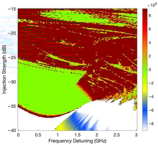
Figure 1.
LLE computed with the Rosenstein method from the optical field amplitude time series . The horizontal axis denotes frequency detuning (GHz), the vertical axis represents injection strength (dB), and the color scale encodes . Each pixel corresponds to a full numerical simulation at the corresponding pair. Positive values (dark-red, red, and orange) indicate chaotic dynamics, values near zero (green) correspond to quasi-periodic behavior, and negative values (blue, yellow, and white regions) represent stable periodic dynamics or non-oscillatory fixed points.
Figure 2 illustrates the core principle of the Rosenstein algorithm for estimating the LLE from a scalar time series. The blue curve represents the average logarithmic divergence between initially nearby trajectories in the reconstructed phase space, tracked over time. According to the method, if the system is chaotic, this divergence should increase exponentially. By taking the logarithm of the separation distance and averaging over multiple trajectory pairs, the method transforms the exponential growth into a linear trend. The red dashed line represents a linear fit to the initial segment of this curve, where the growth is most accurately exponential. The slope of this fit corresponds directly to the LLE, quantifying the rate of separation and thereby the sensitivity to initial conditions. In this case, the positive slope of approximately confirms the presence of chaotic dynamics.
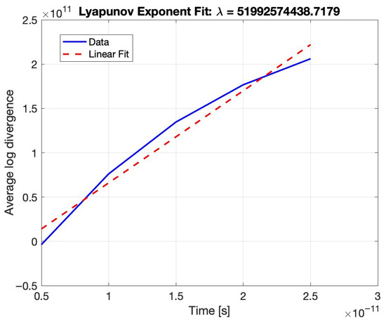
Figure 2.
Average logarithmic divergence of neighboring trajectories over time, estimated from the reconstructed phase space for a power injection ratio of dB and frequency detuning of 1.7 GHz. The blue curve shows the empirical mean log-distance, and the red dashed line is a linear fit over the exponential growth region. The slope yields the positive LLE, confirming chaotic dynamics with sensitivity to initial conditions.
3.2. Results of the LLE Using the Variational Method
To robustly determine the presence of chaos in the OIL system, we implemented a variational Lyapunov exponent analysis based on QR decomposition of the tangent space dynamics, with careful handling of transients and temporal fluctuations. The time evolution of the logarithmic diagonal elements of the R matrix from the QR decomposition, , often exhibits strong oscillatory behavior and lacks pointwise convergence. Rather than relying on a single arbitrary burn-in time to average the exponents, we developed a more systematic and unbiased method: we first identified two sets of indices where —corresponding to the LLE—crosses or approaches zero within a small threshold (e.g., ). The first set is located within the early portion of the simulation (e.g., 20 to 30 ns), and the second set is drawn from the final portion (e.g., 190–200 ns). For each combination of start and end zero-crossings , we compute the average of the cumulative Lyapunov exponent over that interval:
This procedure is repeated for each of the three Lyapunov exponents using the corresponding diagonal elements. The ensemble of estimates is then used to compute the mean and standard deviation of across all combinations. This approach provides a statistically reliable estimate of the dominant Lyapunov exponent while excluding both initial transients and late-stage numerical artifacts. It is particularly effective in systems where weak chaos or intermittent dynamics can lead to misclassification if a single burn-in threshold is applied. We interpret the system as chaotic if the mean of across these intervals is strictly positive and larger than its standard deviation.
Figure 3 shows the parameter map of the LLE computed using the variational method for the OIL system, as a function of frequency detuning (GHz) and injection strength (dB). The color scale represents the magnitude of the Lyapunov exponent, with dark-red, red and orange regions indicating positive values that signify chaotic dynamics, while green regions correspond to near-zero exponents, characteristic of quasi-periodic or weakly unstable oscillations. Negative values, shown in yellow, blue and white, are associated with periodic or stable steady-state behavior. The color scale on the right provides a visual reference for the exponent magnitude, ranging from to . Compared to approximate methods, the variational approach provides a more accurate and fine-grained resolution of the chaotic regions, particularly in the weak-to-moderate injection regime (from dB to dB). The complex fragmentation and layering of chaotic and regular domains highlight the intricate dependence of stability on injection parameters in the OIL dynamics.
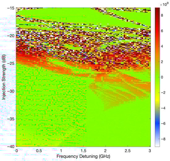
Figure 3.
LLE computed via the variational method. The horizontal axis denotes frequency detuning [GHz], the vertical axis denotes injection strength [dB], and the color scale encodes . The map resolution is 90 points in detuning (≈33 MHz) and 250 points in injection (0.1 dB), for a total of 22,500 simulations. Each pixel corresponds to a full numerical simulation at the parameter pair. Positive values (dark-red–orange) indicate chaotic dynamics, values near zero (green) correspond to quasi-periodic behavior, and negative values (blue–white) represent stable periodic or fixed-point regimes.
Figure 4 shows the Kaplan–Yorke (KY) dimension map for the OIL system, computed from the full Lyapunov spectrum obtained via the variational method. The map is plotted as a function of frequency detuning (GHz) and injection strength (dB). The KY dimension provides an estimate of the fractal dimension of the system’s attractor and serves as a quantitative indicator of chaotic complexity. Regions with a KY dimension close to 1 or higher (depicted in dark-red, red and orange) indicate high-dimensional chaos and a greater number of active degrees of freedom. In contrast, blue and light-blue regions correspond to lower-dimensional attractors, including periodic and quasi-periodic regimes. The presence of intricate filamentary and layered structures suggests a rich interplay between order and chaos across the parameter space. Notably, broad regions of elevated KY dimension are observed in the moderate injection regime ( dB to dB), particularly around detuning values between 1.5 and 2 GHz, highlighting zones of intense chaotic activity.
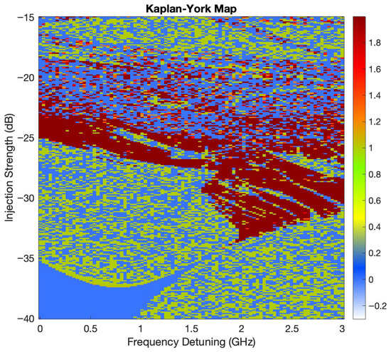
Figure 4.
Kaplan–Yorke (KY) fractal dimension computed from the full Lyapunov spectrum of the OIL system. The horizontal axis denotes frequency detuning (GHz), and the vertical axis denotes injection strength (dB). The color scale represents the KY dimension. For a three-variable model without external delay or feedback, values between 1 and 2 indicate chaotic dynamics. Each pixel represents a full numerical simulation at the corresponding parameter pair.
Figure 5 shows the dissipativity map of the OIL system, with axes representing frequency detuning (GHz) and injection strength (dB). The color scale encodes the time-averaged phase space contraction rate, . Regions in blue to white correspond to high dissipativity, meaning large negative contraction that drives trajectories quickly toward fixed points or stable periodic orbits (locked regimes). In contrast, red and dark-red areas correspond to low dissipativity, where contraction is weak and the system maintains a balance of stretching and folding that allows chaos to persist. In other words, “high dissipativity” here means stronger contraction (more negative), not larger positive values. The map reveals pockets of low-dissipation (chaotic) dynamics embedded within highly dissipative basins, such as the triangular dark-red region near 1.7 GHz detuning and dB injection. By tuning the injection strength to low values ( to dB) and detuning near zero ( GHz, white region), the system naturally falls into the strongly dissipative zones. The numerical grid (90 × 250 points; ≈33 MHz and 0.1 dB, steps) ensures that these narrow bands are resolved with high fidelity.
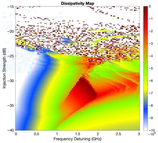
Figure 5.
Dissipativity map of the OIL system. The horizontal axis denotes frequency detuning (GHz), and the vertical axis denotes injection strength (dB). The color scale represents the time-averaged phase space contraction rate, computed along simulated trajectories of the Kobayashi–Lang equations. Blue to white regions correspond to high dissipativity, i.e., strongly negative divergence where trajectories rapidly contract toward fixed points or stable periodic orbits (locked operation). Red regions correspond to low dissipativity, i.e., weak contraction that allows sustained stretching–folding dynamics and thus permits quasi-periodic or chaotic trajectories. Physically, strong dissipativity occurs when the injected field drives to large excursions (rapid carrier depletion) or when aligns for maximal energy transfer from the master laser. The map was obtained on a grid (detuning step MHz, injection step 0.1 dB), with each point integrated for 200 ns at ps, ensuring accurate resolution of the dissipative bands. Each pixel corresponds to a full numerical simulation at the indicated pair.
Across the parameter plane, regions of positive variational LLE in Figure 3 co-localize with weakly dissipative pockets in Figure 5 and with the red bands in Figure 1, confirming that reduced dissipation supports the sustained stretching and folding needed for chaos. Conversely, strongly dissipative zones (blue/white in Figure 5) align with the negative– areas of Figure 1 and Figure 3, indicating periodic or locked operation. This consistency provides a physics-backed rationale for the annotated operating regions.
Figure 6 shows the chaotic attractor of the OIL system in three-dimensional phase space, plotted over the variables , where is the optical field amplitude, the optical phase, and the carrier population. The trajectory exhibits bounded, aperiodic motion with multiple lobes and fine filamentary folding—hallmarks of deterministic chaos. This behavior, obtained at dB injection strength and GHz detuning, is consistent with the computed positive LLE and a Kaplan–Yorke dimension close to 2 (Figure 4). The multi-lobed structure arises from injection-driven phase slippage, which intermittently aligns the coherent drive with the gain window: bursts in are followed by carrier depletion, producing recurrent yet non-repeating dynamics characteristic of a strange attractor. This phase–amplitude interplay provides a mechanistic route to engineer broadband chaos, where increasing the injection ratio enhances amplitude excursions (stronger depletion) and small detuning shifts modulate lobe residence times, thereby shaping spectral flatness and entropy rate.
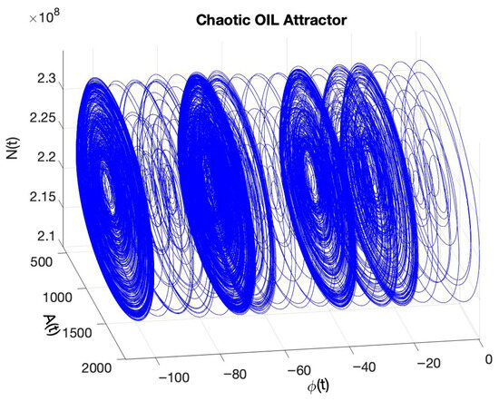
Figure 6.
Chaotic attractor of the OIL system in the three-dimensional phase space spanned by (optical field amplitude), (optical phase), and (carrier density). The trajectory, obtained at dB injection strength and GHz detuning, exhibits bounded, aperiodic motion with filamentary folding and stretching, characteristic of deterministic chaos. These conditions correspond to a positive LLE, a Kaplan–Yorke dimension close to 2, and dissipativity near zero. The attractor geometry reflects the interplay of slow carrier recovery (), rapid photon build-up (), and phase-controlled energy transfer, explaining the broadband spectrum and strong sensitivity to parameter variations observed near this regime.
4. Discussion
Real OIL systems are inherently noisy due to spontaneous emission and Langevin fluctuations, as described in the full Kobayashi–Lang equations. In this study, we intentionally focused on the deterministic, noise-free limit to isolate the intrinsic nonlinear dynamics and to construct high-resolution chaos maps without stochastic variability. This guarantees that the results are exactly reproducible and directly attributable to deterministic mechanisms. While noise in experiments can smooth sharp boundaries and broaden chaotic regions, the underlying bifurcation structures and alternation between stability and chaos remain qualitatively robust. Practical mitigation strategies include ensemble averaging, longer time-series sampling, and noise-reduction schemes. A systematic ensemble-based study of noise effects, together with experimental validation, remains an important avenue for future work.
The structures of alternating stability and chaos bands observed in Figure 1 and Figure 3 are consistent with classical bifurcation analyses [32,38] and are further supported by recent experimental results. For example, Mercadier et al. [39,40] demonstrated that chaos synchronization in cascaded OILs persists across wide bandwidths and parameter variations, validating the robustness of chaotic regimes. Our maps complement such experiments by providing fine-grained numerical diagnostics of the same dynamical transitions.
The explored ranges of injection strength ( to dB) and detuning (0–3 GHz) were chosen to match experimentally realistic configurations reported in previous studies [22,23,24,32]. These conditions include the regions where OILs are known to transition from periodic to chaotic behavior. Other structural parameters such as mirror reflectivity r and injection efficiency were fixed to typical values (Table 1) to enable a high-resolution two-dimensional exploration. A sensitivity analysis of r and , which strongly affect the effective coupling coefficient , is left for future work.
The computed Lyapunov exponents provide a natural classification of attractors: negative corresponds to periodic or locked states, to quasi-periodic behavior, and to chaotic regimes. The Kaplan–Yorke dimension (Figure 4) further confirms low-dimensional chaos in this three-variable model, while the dissipativity map (Figure 5) distinguishes strongly contracting basins (stable/locked) from weakly contracting, chaos-permissive regions. Because it is not feasible to show attractors for all grid points, a representative chaotic trajectory is included in Figure 6, visually confirming the multi-lobed, aperiodic structure predicted by Lyapunov indicators. Together, these complementary measures establish a consistent and quantitative classification of dynamical regimes.
The feasibility of validating these maps experimentally has already been demonstrated in our earlier work on pulsing regimes of OILs [22]. That master–slave setup with time-domain detection can be directly adapted to chaos validation: by recording sufficiently long intensity traces of the slave laser and processing them with Lyapunov-based algorithms (e.g., Rosenstein or lyapunovExponent.m), one can experimentally extract and compare it to the deterministic maps reported here. While this paper focuses on theory and numerical simulations, such experimental validation represents a natural continuation.
Broader implications and future work. The high-resolution chaos maps developed here are directly relevant to applications requiring controllable nonlinear dynamics. In secure communications, they enable systematic configuration of chaos-based encryption links; in random number generation, they identify broadband chaotic windows for maximizing entropy; and in neuromorphic computing, the reproducibility and low-dimensional nature of OIL chaos make them promising candidates for photonic reservoir computing. Another important direction is the integration of OIL-based chaos sources into silicon photonics platforms. In particular, photonic wires in CMOS-compatible PICs allow co-integration of semiconductor lasers with key functional blocks such as optical isolators, variable optical attenuators, polarization controllers, and high-speed photodetectors, providing a pathway toward fully integrated chaos-enabled transmitters [11]. These perspectives underscore the versatility of OILs as a photonic platform for both fundamental studies and applied technologies.
5. Conclusions
OILs display a wide variety of dynamical regimes—including periodic, quasi-periodic, and chaotic states—that depend sensitively on injection strength and frequency detuning. A persistent challenge has been the absence of reproducible, high-resolution maps that delineate these regimes and enable their systematic exploitation.
In this work, we addressed this problem using a deterministic, noise-free version of the Kobayashi–Lang equations, which isolates the intrinsic nonlinear dynamics by eliminating stochastic fluctuations. This modeling choice avoids ambiguity and ensures reproducibility of the observed structures. To quantify sensitivity to initial conditions and rigorously detect chaos, we employed two complementary methods for computing the LLE: the Rosenstein time-delay embedding method, well suited for short experimental time series, and a variational technique that integrates the tangent space dynamics. Their agreement provides robust cross-validation and fine-grained resolution of chaotic domains.
By jointly analyzing the Rosenstein LLE map (Figure 1), the exact variational LLE map (Figure 3), and the dissipativity map (Figure 5), we established a direct feedback loop between figures and device operation. Positive LLE bands identify injection–detuning pairs that produce broadband chaos, while highly dissipative basins predict stable periodic or locked behavior. Practically, selecting to dB injection with detuning near the identified red bands yields robust chaos generation; operating at lower injection or within blue–white basins favors stability for communications. These figure-informed prescriptions turn the maps into actionable design tools for OIL-based systems.
The main contributions of this study are therefore (i) construction of high-resolution chaos maps in the injection–detuning plane; (ii) cross-validated Lyapunov analysis combining Rosenstein and variational methods; and (iii) integration of dissipativity measures to provide physical intuition on stability. The key findings include the identification of parameter windows for controllable chaos generation versus stable locked operation, as well as quantitative classification of attractors through Lyapunov spectra and Kaplan–Yorke dimension.
A deliberate methodological choice in this work was to restrict the analysis to the deterministic limit of the Kobayashi–Lang equations. By eliminating stochastic contributions, the resulting chaos maps are fully reproducible and reflect only the intrinsic nonlinear dynamics of the system, without ambiguity from noise-induced fluctuations or apparent “false chaos.” Real OILs are of course noisy, and future extensions should incorporate ensemble-based stochastic simulations and experimental validation.
Looking forward, the present methodology provides a reproducible foundation for exploring photonic chaos. Extending it to delayed-feedback configurations could reveal hyperchaotic attractors of higher dimensionality, while experimental verification under noisy conditions will strengthen practical relevance. Finally, integration of OIL-based chaos sources into silicon photonic platforms represents a promising path toward applications in secure communications, photonic random number generation, and neuromorphic photonics.
Author Contributions
Writing—review & editing, G.A.C.Á.; validation, A.A.-Z.; formal analysis, I.A. and A.M.S.-M. All authors have read and agreed to the published version of the manuscript.
Funding
This research was funded by Secretaría de Ciencia, Humanidades, Tecnología e Innovación (SeCiHTI).
Data Availability Statement
Data underlying the results presented in this paper are not publicly available at this time but may be obtained from the authors upon reasonable request.
Conflicts of Interest
The authors declare no conflicts of interest.
References
- Wang, A.; Wang, J.; Jiang, L.; Wang, L.; Wang, Y.; Yan, L.; Qin, Y. Experimental demonstration of 8190-km long-haul semiconductor-laser chaos synchronization induced by digital optical communication signal. Light Sci. Appl. 2025, 14, 40. [Google Scholar] [CrossRef]
- Zhang, M.; Wang, Y. Review on Chaotic Lasers and Measurement Applications. J. Light. Technol. 2021, 39, 3711–3723. [Google Scholar] [CrossRef]
- Yu, F.; He, T.; He, S.; Tan, B.; Shi, C.; Lin, H. Influence of Memristive Activated Gradient on Chaotic Dynamics in Discrete Neural Networks. Int. J. Bifurc. Chaos 2024, 35, 2550146. [Google Scholar] [CrossRef]
- Yu, F.; He, S.; Yao, W.; Cai, S.; Xu, Q. Bursting Firings in Memristive Hopfield Neural Network with Image Encryption and Hardware Implementation. IEEE Trans. Comput.-Aided Des. Integr. Circuits Syst. 2025, 1. [Google Scholar] [CrossRef]
- Feng, W.; Zhang, K.; Zhang, J.; Zhao, X.; Chen, Y.; Cai, B.; Zhu, Z.; Wen, H.; Ye, C. Integrating Fractional-Order Hopfield Neural Network with Differentiated Encryption: Achieving High-Performance Privacy Protection for Medical Images. Fractal Fract. 2025, 9, 426. [Google Scholar] [CrossRef]
- Li, H.; Yu, S.; Feng, W.; Chen, Y.; Zhang, J.; Qin, Z.; Zhu, Z.; Wozniak, M. Exploiting Dynamic Vector-Level Operations and a 2D-Enhanced Logistic Modular Map for Efficient Chaotic Image Encryption. Entropy 2023, 25, 1147. [Google Scholar] [CrossRef]
- Ashok, P.; Ganesh Madhan, M.; Deepiha, P.; Rimmya, C.; Piramasubramanian, S. An Efficient Chaotic Optical signal generation scheme using Gain Lever Effect in bi-section laser diodes. Opt. Commun. 2020, 475, 126202. [Google Scholar] [CrossRef]
- Li, X.Z.; Chan, S.C. Random bit generation using an optically injected semiconductor laser in chaos with oversampling. Opt. Lett. 2012, 37, 2163–2165. [Google Scholar] [CrossRef] [PubMed]
- Yu, Q.; Chen, H.; Sun, X.; Tan, M.; Li, Y.; Xu, Z.; Pan, S. Ultra-broadband chaotic laser and microwave ranging based on an optoelectronic oscillator. Opt. Lett. 2025, 50, 3557–3560. [Google Scholar] [CrossRef] [PubMed]
- Mu, X.; Yan, Z.; Yu, Y.; Yan, H.; Han, D. A tunable self-mixing chaotic laser based on high frequency electro-optic modulation. Opt. Laser Technol. 2020, 127, 106172. [Google Scholar] [CrossRef]
- Castañón, G.; Cerroni, W.; Sarmiento-Moncada, A.M. Integrated Photonics for IoT, RoF, and Distributed Fog–Cloud Computing: A Comprehensive Review. Appl. Sci. 2025, 15, 7494. [Google Scholar] [CrossRef]
- Zeng, Y.; Zhou, P.; Huang, Y.; Li, N. Optical chaos generated in semiconductor lasers with intensity-modulated optical injection:a numerical study. Appl. Opt. 2021, 60, 7963–7972. [Google Scholar] [CrossRef]
- Li, J.C.; Xiao, J.L.; Yang, Y.D.; Chen, Y.L.; Huang, Y.Z. Random bit generation based on a self-chaotic microlaser with enhanced chaotic bandwidth. Nanophotonics 2023, 12, 4109–4116. [Google Scholar] [CrossRef]
- Wang, X.; Zheng, T.; Jia, Y.; Huang, J.; Zhu, X.; Shi, Y.; Wang, N.; Lu, Z.; Zou, J.; Li, Y. Compact Quantum Random Number Generator Based on a Laser Diode and a Hybrid Chip with Integrated Silicon Photonics. Photonics 2024, 11, 468. [Google Scholar] [CrossRef]
- Shen, B.; Shu, H.; Xie, W.; Chen, R.; Liu, Z.; Ge, Z.; Zhang, X.; Wang, Y.; Zhang, Y.; Cheng, B.; et al. Harnessing microcomb-based parallel chaos for random bit generation in integrated photonics. Nat. Commun. 2023, 14, 4590. [Google Scholar] [CrossRef]
- Inoue, S.; Kanno, K.; Uchida, A. Prevention of Intermittent Chaos in Semiconductor Laser with Optical Feedback. In Proceedings of the 2022 Conference on Lasers and Electro-Optics Pacific Rim, Sapporo, Japan, 31 August–5 September 2022; Optica Publishing Group: Washington, DC, USA, 2022; pp. 1–3. [Google Scholar] [CrossRef]
- Spitz, O.; Herdt, A.; Wu, J.; Maisons, G.; Carras, M.; Wong, C.W.; Elsäßer, W.; Grillot, F. Private communication with quantum cascade laser photonic chaos. Nat. Commun. 2021, 12, 3327. [Google Scholar] [CrossRef]
- Xie, Y.; Yang, Z.; Shi, M.; Zhuge, Q.; Hu, W.; Yi, L. 100 Gb/s coherent chaotic optical communication over 800 km fiber transmission via advanced digital signal processing. Adv. Photonics Nexus 2023, 3, 016003. [Google Scholar] [CrossRef]
- Wang, Z.; Shen, L.; Yang, M.; Tang, Z.; Zhang, L.; Yan, C.; Yang, L.; Wang, R.; Chu, J.; Du, J.; et al. High-speed chaos-based secure optical communications over 130-km multi-core fiber. Opt. Lett. 2023, 48, 4440–4443. [Google Scholar] [CrossRef]
- Feng, J.; Jiang, L.; Sun, J.; He, X.; Yi, A.; Pan, W.; Yan, L. 256 Gbit/s Chaotic Optical Communication over 1600 Km Using an AI-based Optoelectronic Oscillator Model. J. Light. Technol. 2024, 42, 2774–2783. [Google Scholar] [CrossRef]
- Mao, X.; Wang, A.; Wang, L.; Fu, S.; Wang, Y.; Qin, Y. 100-Gbit/s 100-km Physical-Layer Secure Fiber-Optic Communication Using Wideband Chaotic Semiconductor Lasers. J. Light. Technol. 2025, 43, 2176–2183. [Google Scholar] [CrossRef]
- Aldaya, I.; Campuzano, G.; Castañón, G.; Gosset, C.; Wang, C.; Grillot, F. Periodic and aperiodic pulse generation using optically injected DFB laser. Electron. Lett. 2015, 51, 280–282. [Google Scholar] [CrossRef]
- Rodriguez, S.; Campuzano, G.; Aldaya, I.; Castañón, G. Numerical analysis of pulsing regimes near static borders of optically injected semiconductor lasers. Appl. Opt. 2022, 61, 2634–2643. [Google Scholar] [CrossRef] [PubMed]
- Castañón, G.A.; Rodriguez, S.; Campuzano, G.; Aldaya, I. Numerical analysis of the impact of noise in pulsing regimes generated using optically injected lasers. Appl. Opt. 2025, 64, 5344–5349. [Google Scholar] [CrossRef]
- Rosenstein, M.T.; Collins, J.J.; De Luca, C.J. A practical method for calculating largest Lyapunov exponents from small data sets. Phys. D Nonlinear Phenom. 1993, 65, 117–134. [Google Scholar] [CrossRef]
- Sciamanna, M.; Shore, K.A. Physics and applications of laser diode chaos. Nat. Photonics 2015, 9, 151–162. [Google Scholar] [CrossRef]
- Lau, E. High-Speed Modulation of Semiconductor Lasers by Optical Injection Locking; VDM: Saarbrücken, Germany, 2008. [Google Scholar]
- Murakami, A.; Kawashima, K.; Atsuki, K. Cavity resonance shift and bandwidth enhancement in semiconductor lasers with strong light injection. IEEE J. Quantum Electron. 2003, 39, 1196–1204. [Google Scholar] [CrossRef]
- Wieczorek, S.; Krauskopf, B.; Lenstra, D. A unifying view of bifurcations in a semiconductor laser subject to optical injection. Opt. Commun. 1999, 172, 279–295. [Google Scholar] [CrossRef]
- Sivaprakasam, S.; Shore, K. Demonstration of optical synchronization of chaotic external-cavity laser diodes. Opt. Lett. 1999, 24, 466–468. [Google Scholar] [CrossRef]
- Mirasso, C.; Colet, P.; Garcia-Fernandez, P. Synchronization of chaotic semiconductor lasers: Application to encoded communications. IEEE Photonics Technol. Lett. 1996, 8, 299–301. [Google Scholar] [CrossRef]
- Osinski, M.; Buus, J. Linewidth broadening factor in semiconductor lasers–An overview. IEEE J. Quantum Electron. 1987, 23, 9–29. [Google Scholar] [CrossRef]
- Takens, F. Detecting strange attractors in turbulence. In Dynamical Systems and Turbulence, Warwick 1980; Rand, D., Young, L.S., Eds.; Lecture Notes in Mathematics; Springer: Berlin/Heidelberg, Germany, 1981; Volume 898, pp. 366–381. [Google Scholar] [CrossRef]
- Kennel, M.B.; Brown, R.; Abarbanel, H.D.I. Determining embedding dimension for phase-space reconstruction using a geometrical construction. Phys. Rev. A 1992, 45, 3403–3411. [Google Scholar] [CrossRef]
- Benettin, G.; Galgani, L.; Giorgilli, A.; Strelcyn, J.M. Lyapunov characteristic exponents for smooth dynamical systems and for Hamiltonian systems; a method for computing all of them. Part 1: Theory. Meccanica 1980, 15, 9–20. [Google Scholar] [CrossRef]
- Skokos, C. The Lyapunov characteristic exponents and their computation. Lect. Notes Phys. 2010, 790, 63–135. [Google Scholar] [CrossRef]
- Kaplan, J.; Yorke, J.A. Chaotic behavior of multidimensional difference equations. In Functional Differential Equations and Approximations of Fixed Points: Proceedings, Bonn, July 1978; Peitgen, H.O., Walther, H.O., Eds.; Springer: Berlin/Heidelberg, Germany, 1979; pp. 204–227. [Google Scholar]
- Wieczorek, S.; Krauskopf, B.; Simpson, T.; Lenstra, D. The dynamical complexity of optically injected semiconductor lasers. Phys. Rep. 2005, 416, 1–128. [Google Scholar] [CrossRef]
- Mercadier, J.; Doumbia, Y.; Bittner, S.; Sciamanna, M. Optical chaos synchronization in a cascaded injection experiment. Opt. Lett. 2024, 49, 2613–2616. [Google Scholar] [CrossRef]
- AlMulla, M. Featureless Broadband Chaos Through Cascaded Optically Injected Semiconductor Lasers. Photonics 2025, 12, 325. [Google Scholar] [CrossRef]
Disclaimer/Publisher’s Note: The statements, opinions and data contained in all publications are solely those of the individual author(s) and contributor(s) and not of MDPI and/or the editor(s). MDPI and/or the editor(s) disclaim responsibility for any injury to people or property resulting from any ideas, methods, instructions or products referred to in the content. |
© 2025 by the authors. Licensee MDPI, Basel, Switzerland. This article is an open access article distributed under the terms and conditions of the Creative Commons Attribution (CC BY) license (https://creativecommons.org/licenses/by/4.0/).