Assessment of Transformer Fault Severity from Online Dissolved Gas Analysis Using Positive CUSUM

Abstract

Dissolved gas analysis (DGA) is one of the transformer testing methods that has been widely used for a long time because it does not require the transformer to be offline for testing. The inspection can be conducted while the transformer is operating normally, and it is cost-effective. In research on fault severity, thermodynamic theory has been applied to find the energy index of the hydrocarbon gases generated by faults, ${\mathrm{CH}}_4$, ${\mathrm{C}}_2{\mathrm{H}}_6$, ${\mathrm{C}}_2{\mathrm{H}}_4$ and ${\mathrm{C}}_2{\mathrm{H}}_2$, referred to as the Normalised Energy Intensity (NEI). This study examines the application of the Positive Cumulative Sum of Difference (CUSUM) method to hydrocarbon NEI and carbon dioxide NEI for fault severity assessment. The study demonstrates the effectiveness of this approach by means of case studies on the basis of DGA results from two steel plants. In the case of NEI from hydrocarbon gases (${\mathrm{NEI}}_{\mathrm{HC}}$), the positive CUSUM is compared with the NEI, the NEI score, and the cumulative NEI. In the case of NEI from carbon oxide gases (${\mathrm{NEI}}_{\mathrm{CO}}$), Positive CUSUM is compared with NEI and the ratio of ${\mathrm{CO}}_2$ to $\mathrm{CO}$. It was found that Positive CUSUM for ${\mathrm{NEI}}_{\mathrm{HC}}$ is a much better indicator of the severity of defects than the NEI, the NEI score, and the cumulative NEI. In contrast, Positive CUSUM for ${\mathrm{NEI}}_{\mathrm{CO}}$ gave excessively high values. However, combining NEI with the ${\mathrm{CO}}_2$/$\mathrm{CO}$ ratio gave better monitoring results. Therefore, from an online DGA perspective, Positive CUSUM can be used to effectively monitor fault severity.

1. Introduction

Transformers are essential devices in power generation, transmission, and distribution systems, affecting the stability and reliability of the electrical system. The continuous operation of transformers is therefore crucial for electric utilities and electricity consumers. A fault within a transformer can disrupt the stability and reliability of the power system. The continuous operation of transformers is therefore crucial for utilities and their users. Problems within the transformer, however, can lead to the impairment of a vital and costly component of the power distribution system. Certain types of faults may escalate into catastrophic events, causing substantial destruction to nearby equipment and posing risks to individuals. Maintenance of electrical transformers at the onset of damage is necessary. Routine maintenance once a year and sampling of dielectric fluid for dissolved gas analysis may not be sufficient for assessing the health of heavily used transformers in plants.

These plants opt for online dissolved gas analyzers in transformer oil. This provides continuous observation and assessment of the transformer’s condition. This allows them to make prompt decisions if abnormalities arise because of internal faults. Since the relationship between transformer faults and combustible gases from oil decomposition was discovered, extensive research has been conducted to identify the types and quantities of these gases. Dissolved gas analysis has a long history, dating back to the 1960s [1], while online dissolved gas analyzers for transformer oil, manufactured by Morgan Schaffer [2], were first used in the 1970s. Dissolved gas analysis has been used to distinguish between transformers operating normally and those exhibiting abnormalities and to pinpoint the nature of these abnormalities. These analytical methods emerged during the 1970s to 1990s, such as the Doernenburg Ratios [3], Rogers Ratios [4], and Duval Triangles [5,6]. IEC 60599 and IEEE C57.104 [7,8], developed in 1977–1978, provide standards for interpreting dissolved gas analysis results. These standards were created by a group of experts using data collected from transformer oil. These two standards serve as the basis for interpretation and have been regularly updated for the present in the form of IEC 60599-2022 and IEEE C57.104-2019 [9,10]. The approach to assessing the severity of faults based on dissolved gas analysis (DGA) begins with the concept of prioritizing maintenance for transformers.

2. Normalized Energy Intensity (NEI)

Research by Jakob and Dukarm first presented the NEI in 2015 [11,12], using the concentrations of gases and the enthalpy values of the gases ${\mathrm{CH}}_4$, ${\mathrm{C}}_2{\mathrm{H}}_6$, ${\mathrm{C}}_2{\mathrm{H}}_4$, and ${\mathrm{C}}_2{\mathrm{H}}_2$ from n-octane (${\mathrm{C}}_8{\mathrm{H}}_{18}$) to calculate the NEI that directly reflects the energy from faults occurring in transformers. The equation for NEI from hydrocarbon gases (${\mathrm{NEI}}_{\mathrm{HC}}$) is as follows:

$$NE{I}_{HC}={\displaystyle \frac{77.7C{H}_4+93.5C_2{H}_6+104.1C_2{H}_4+278.3C_2{H}_2}{22400}}$$

(1)

The IEEE C57.104-2019 standard has incorporated the Normalized Energy Intensity (NEI) from the concentrations of carbon monoxide and carbon dioxide gases (${\mathrm{NEI}}_{\mathrm{CO}}$) produced by faults affecting solid insulation, particularly the paper wrapping around windings. This value can effectively monitor the degradation of solid insulation, since both types of carbon oxide gases usually occur gradually. The equation for ${\mathrm{NEI}}_{\mathrm{CO}}$ is

$$NE{I}_{CO}={\displaystyle \frac{101.4CO+30.2C{O}_2}{22400}}$$

(2)

The IEEE standard also provides a detailed correlation between the ${\mathrm{NEI}}_{\mathrm{CO}}$ value and the ${\mathrm{CO}}_2/\mathrm{CO}$ ratio. It specifically states that a fault affecting paper insulation has occurred if the ${\mathrm{NEI}}_{\mathrm{CO}}$ value exhibits a rapid increase while the ${\mathrm{CO}}_2/\mathrm{CO}$ ratio decreases. This information is of paramount importance for monitoring the severity of faults from online DGA measuring devices.

3. Assessment of Fault Severity from NEI

The approach to classifying severity based on dissolved gases’ analysis from transformer oil samples began with the research of John Lapworth, who used a scoring system for DGA results to help prioritize the abnormalities that occur. This method provides a more precise representation of developing issues within transformers and helps to consistently and reliably assess the health of transformer groups.

Research by Jakob and Dukarm presents the Normalized Energy Intensity (NEI) by considering the energy values of gases generated from faults to analyze the severity of the occurring faults. The NEI assigns a score known as the ‘NEI score,’ categorizing severity into four levels according to IEEE and IEC styles. Transformers are classified into high- and low-oxygen types based on the ${\mathrm{N}}_2/{\mathrm{O}}_2$ ratio; if the value is greater than 5.94, it is considered a low-oxygen transformer, while a value less than 5.94 indicates a high-oxygen type. The NEI limits on the 90th, 95th, and 98th percentile are as per

Table 1. NEI limits based on 90th, 95th, 98th percentiles of data.

Group	${\mathbf{L}}_1$	${\mathbf{L}}_2$	${\mathbf{L}}_3$
High-${\mathrm{O}}_2$	0.39	0.72	1.98
Low-${\mathrm{O}}_2$	1.02	1.87	4.00

.

Assuming the calculated NEI value equals x, we can calculate the oil sample’s NEI value using hydrocarbon gas concentrations and then determine the NEI score by following these steps.

• If x > $L_3$, the NEI Score is 4.0.
• If $L_2$⩽ x< $L_3$, the NEI Score is ${\displaystyle 3+\frac{x-L_2}{L_3-L_2}}$.
• If $L_1$⩽ x< $L_2$, the NEI Score is ${\displaystyle 2+\frac{x-L_1}{L_2-L_1}}$.
• If x < $L_1$, the NEI Score is ${\displaystyle 1+\frac{x}{L_1}}$.

While the NEI score effectively ranks the fault severity, there are still questions about the applicability of its limits to transformers with different applications, such as those used in steel melting plants. Can these limits be applied to environmental conditions in other regions?

Several subsequent research studies have utilized the NEI to assess the severity of faults occurring within transformers [13,14,15,16]. The IEEE C57.104-2019 standard introduced the NEI in Annex F [10] as an alternative for analyzing the severity of faults occurring within transformers by incorporating the NEI of cellulose insulation that produces carbon dioxide (${\mathrm{CO}}_2$) and carbon monoxide ($\mathrm{CO}$).

Dukarm and Draper proposed a method for tracking NEI values using cumulative sums [17]. If the next value increases, the difference is added to the previous value; if the next value is lower than the previous one, it remains unchanged.

4. Statistical Process Control (SPC)

A longstanding technique widely applied in industrial manufacturing for controlling production processes is Statistical Process Control (SPC). Walter A. Shewhart developed the control chart in 1924 [18,19,20]. It is one of the seven essential SPC tools for monitoring production process changes.

Because Shewhart control charts are insensitive to small process shifts, the CUSUM chart was developed for quality control. First proposed in 1958 by Page [21,22,23], this method has seen continuous application and study across various fields. These include energy savings in industrial processes [24], electrical system parameter monitoring for modeling [25], and analysis of PM2.5 dust levels following changes to natural gas usage [26].

CUSUM charts suit online transformer measurement because of continuous data alignment with CUSUM principles. For example, they can detect abnormalities in transformer windings and identify faults in transformer coils. The Positive CUSUM presented in this article is the part of a cumulative sum (CUSUM) chart that considers only the positive deviations from a baseline value. It is designed to quickly and accurately detect increases in the NEI value, which reflects the severity of faults in transformers. Monitoring with this value is important for industrial plants that have high transformer load usage, such as steel mills.

The faults within the transformer generate various types of gases, primarily flammable gases. This research utilizes the correlation of Total Dissolved Combustible Gas (TDCGs), found in the DGA online measurement devices’ data, with NEI values in order to derive a linear regression equation and ${\mathrm{R}}^2$. If we use the TDCG values directly, there will be a significant difference between the minimum and maximum values. Using the logarithm of TDCG helps to mitigate the impact of data skewness, making the linear regression model more suitable.

5. Methodology for Using Positive CUSUM

This research article presents the use of Positive CUSUM of the NEI value for monitoring the severity of faults. The steps for implementing Positive CUSUM are as follows:

• Extract the DGA data of nine gases from the online measurement device, remove non-numeric values, and separate it into 12 months.
• Calculate the logarithm of the total dissolved combustible gas (TDCG).
• Find the values of ${\mathrm{NEI}}_{\mathrm{HC}}$ and ${\mathrm{NEI}}_{\mathrm{CO}}$ for each month.
• Create a scatter plot between log(TDCG) and NEI.
• A linear regression of log(TDCG) against NEI will identify the month exhibiting the strongest correlation (highest ${\mathrm{R}}^2$), which will then serve as the baseline for a linear equation:

  $$\begin{array}{c}\hfill NE{I}_{predict}=m\times log\left(TDCG\right)+c\end{array}$$

  (3)
• Calculate the forecast NEI values (${\mathrm{NEI}}_{\mathrm{Predict}}$) of each data point with the base month equation.
• Compute the discrepancy ($\mathrm{Diff}$) between measured NEI (${\mathrm{NEI}}_{\mathrm{Data}}$) and predicted NEI (${\mathrm{NEI}}_{\mathrm{Predict}}$).

  $$\begin{array}{c}\hfill Diff=NE{I}_{Data}-NE{I}_{predict}\end{array}$$

  (4)
• Calculate the Positive CUSUM (Pos. CUSUM).

  $$\begin{array}{c}\hfill Pos.CUSU{M}_0=0\end{array}$$

  (5)

  $$\begin{array}{c}\hfill Pos.CUSU{M}_i=Pos.CUSU{M}_{i-1}+Dif{f}_i\end{array}$$

  (6)

  $$\begin{array}{c}\hfill IFPos.CUSU{M}_i<0THENPos.CUSU{M}_i=0\\ \hfill ELSEPos.CUSU{M}_i\end{array}$$

  (7)
• Create a Positive CUSUM chart.
• Generate a graphical representation comparing NEI values, Positive CUSUM, NEI score, and cumulative NEI.

Positive CUSUM’s straightforward calculation makes it ideal for online DGA devices that are continuously monitoring critical transformers in production lines. Positive CUSUM is sensitive to changes, thus yielding results that clearly show differences. The following section will illustrate the application of Positive CUSUM using data from online dissolved gas analysis (DGA) devices from two steel mills.

6. Case Study

6.1. Transformer in the Steel Industry 1

A steel factory uses a 130 MVA Arc Furnace transformer with a rated voltage of 33/1.25 kV, manufactured in 1997. The transformer uses a Morgan Schaffer brand online DGA monitor Model Calisto R9, as shown in Figure 1. This device measures nine gases (${\mathrm{H}}_2$, ${\mathrm{CH}}_4$, ${\mathrm{C}}_2{\mathrm{H}}_6$, ${\mathrm{C}}_2{\mathrm{H}}_4$, ${\mathrm{C}}_2{\mathrm{H}}_2$, $\mathrm{CO}$, ${\mathrm{CO}}_2$, ${\mathrm{O}}_2$, ${\mathrm{N}}_2$) and records concentrations every four hours. The sample data is shown in

Table 2. Sample DGA results from the steel factory in Case Study 1.

Time	${\mathbf{H}}_2$ (ppm)	${\mathbf{CH}}_4$ (ppm)	${\mathbf{C}}_2{\mathbf{H}}_6$ (ppm)	${\mathbf{C}}_2{\mathbf{H}}_4$ (ppm)	${\mathbf{C}}_2{\mathbf{H}}_2$ (ppm)	$\mathbf{CO}$ (ppm)	${\mathbf{CO}}_2$ (ppm)	${\mathbf{O}}_2$ (ppm)	${\mathbf{N}}_2$ (ppm)	TDCG (ppm)
1 January 2023 02:10	37	111	46.4	195	6.4	166	1290	18,500	41,000	561.8
1 January 2023 06:10	37	111	46.2	194	6.4	164	1280	18,700	41,000	558.6
1 January 2023 10:10	37	111	46.4	195	6.4	164	1290	18,600	40,000	559.8
1 January 2023 14:10	36.5	111	46.2	194	6.4	164	1290	18,600	41,000	558.1
1 January 2023 18:10	37	111	46.2	194	6.4	164	1290	18,700	41,000	558.6
1 January 2023 22:10	37	112	46.2	196	6.4	168	1310	20,100	41,000	565.6
2 January 2023 02:10	37	114	46.6	198	6.6	170	1330	20,300	41,000	572.2
2 January 2023 06:10	37.5	113	46.8	198	6.6	170	1330	20,500	41,000	571.9

. The DGA results from January to December 2023 of gases ${\mathrm{H}}_2$, ${\mathrm{CH}}_4$, ${\mathrm{C}}_2{\mathrm{H}}_6$, ${\mathrm{C}}_2{\mathrm{H}}_4$, ${\mathrm{C}}_2{\mathrm{H}}_2$, $\mathrm{CO}$, ${\mathrm{CO}}_2$, ${\mathrm{O}}_2$, ${\mathrm{N}}_2$ and TDCG are shown.

From Figure 2, it can be observed that there were abnormal data during the period from 13 February 2023 to 10 March 2023 due to an unusual decrease in DGA values. This was caused by the online DGA analyzer reporting lower-than-normal values for some gases. Therefore, the analysis needs to be divided into two periods: January to February and March to December.

Utilize the DGA data obtained from the online measuring device to execute the following steps.

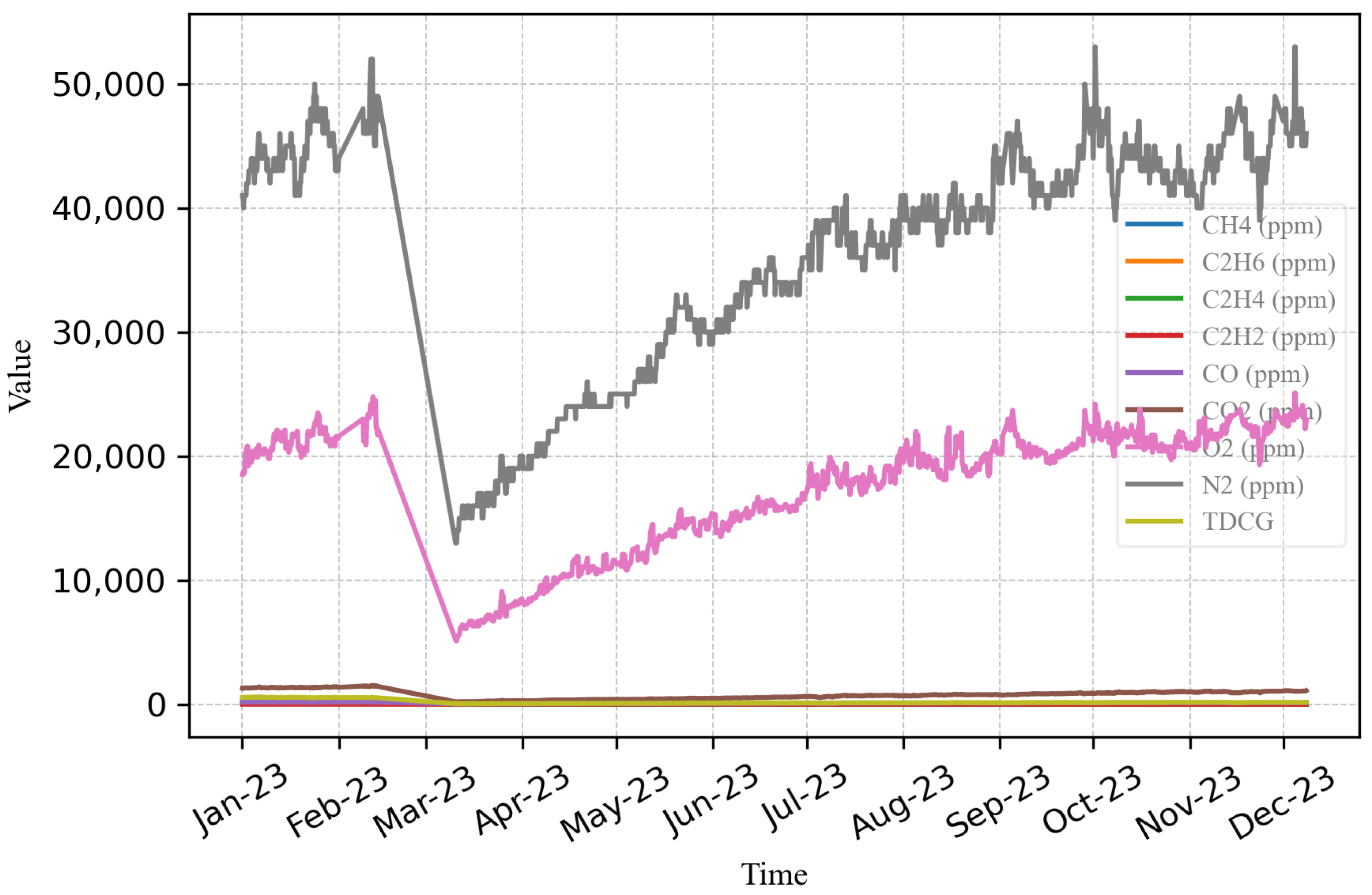
• Take the data from January to February and March to December 2023 for all nine types of gas, at 4 h intervals. Remove the data points that lack complete information.
• Determine the total dissolved combustible gas (TDCG) and calculate its logarithmic value.
• Calculate the value of ${\mathrm{NEI}}_{\mathrm{HC}}$ using the equation provided in (1) and the value of ${\mathrm{NEI}}_{\mathrm{CO}}$ using the equation provided in (2). The chemical formula of the gas in the equation indicates its concentration under standard temperature and pressure conditions (273.15 K and 101.325 kPa).

  Table 3. The values of log(TDCG), ${\mathrm{NEI}}_{\mathrm{HC}}$, ${\mathrm{NEI}}_{\mathrm{CO}}$ and ${\mathrm{CO}}_2$/CO ratio.

  Time	log(TDCG)	${\mathbf{NEI}}_{\mathbf{HC}}$	${\mathbf{NEI}}_{\mathbf{CO}}$	${\mathbf{CO}}_2$/CO
  1 January 2023  02:10	2.750	1.564	2.491	7.771
  1 January 2023 06:10	2.747	1.559	2.468	7.805
  1 January 2023 10:10	2.750	1.564	2.482	7.866
  1 January 2023 14:10	2.750	1.564	2.482	7.866
  1 January 2023 18:10	2.750	1.564	2.482	7.866
  1 January 2023 22:10	2.750	1.564	2.527	7.798
  2 January 2023 02:10	2.750	1.564	2.563	7.824
  2 January 2023 06:10	2.750	1.564	2.563	7.824

  presents the values of log(TDCG), ${\mathrm{NEI}}_{\mathrm{HC}}$, ${\mathrm{NEI}}_{\mathrm{CO}}$ and ${\mathrm{CO}}_2/\mathrm{CO}$ ratio.
• The data obtained from step 3 are segmented into monthly data sets.

Evaluate the NEI of hydrocarbon gas from January to February

• Determine the correlation between the log(TDCG) and the ${\mathrm{NEI}}_{\mathrm{HC}}$ using linear regression to calculate the coefficient of determination (${\mathrm{R}}^2$) for each month, as illustrated in

  Table 4. The Correlation coefficient of Hydrocarbon Gas from January to December 2023.

  January	February	March	April	May	June
  0.8926	0.9706	0.578	0.7969	0.7745	0.7317
  July	August	September	October	November	December
  0.8532	0.4454	0.6659	0.6396	0.1294	0.1292

  . It was discovered that February had the highest ${\mathrm{R}}^2$ value of 0.9706. The linear equation derived from the linear regression, presented in Figure 3, is

  $$NE{I}_{Predict}=1.4306\times log\left(TDCG\right)-2.4192$$

  (8)
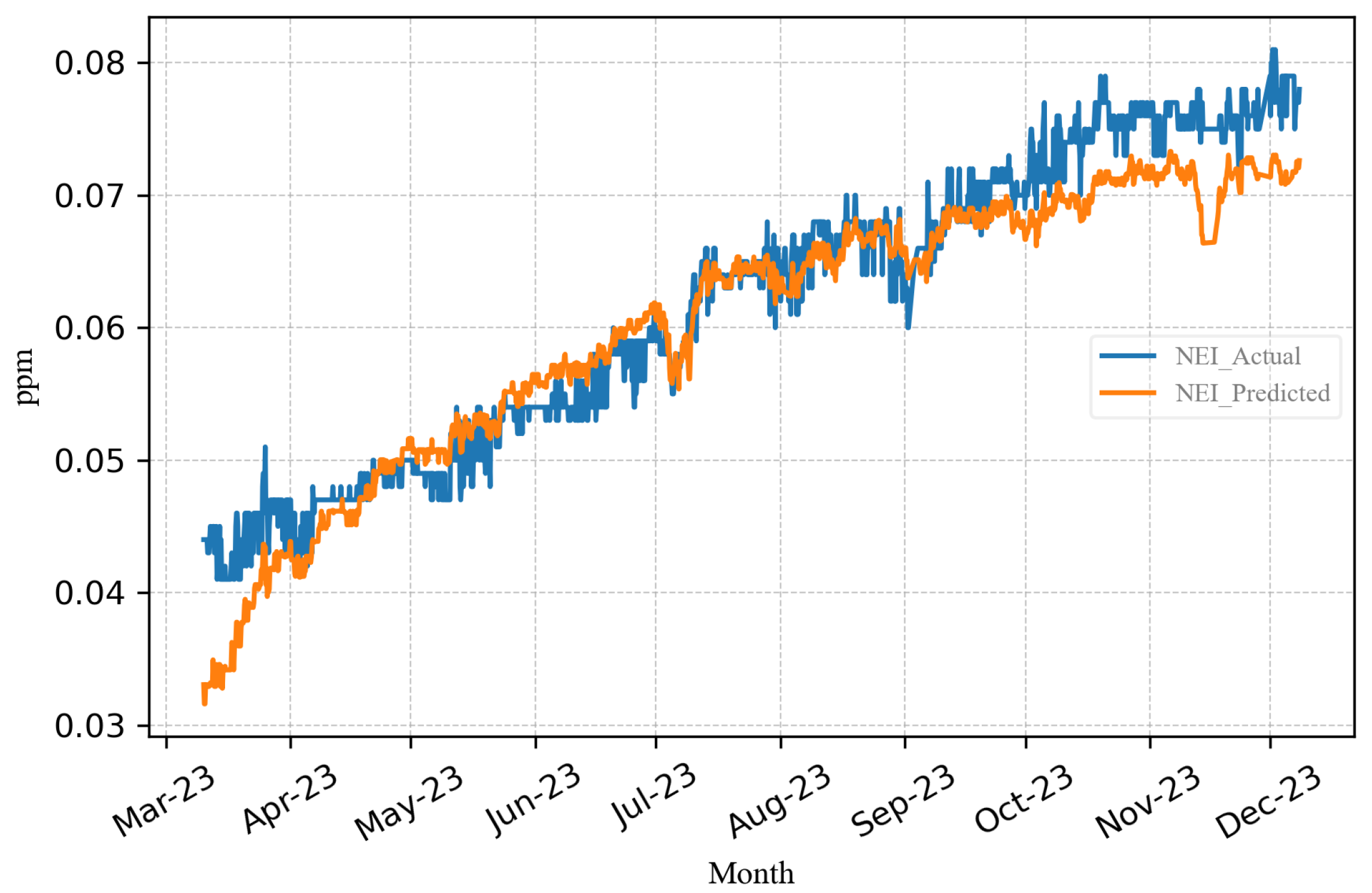
• Determine the difference (Diff) between the NEI data obtained from the DGA results and the NEI data calculated using the baseline equation, and calculate the CUSUM from the equation.

  $$CUSUM=\sum _1^n{\left(Diff\right)}_i$$

  (9)
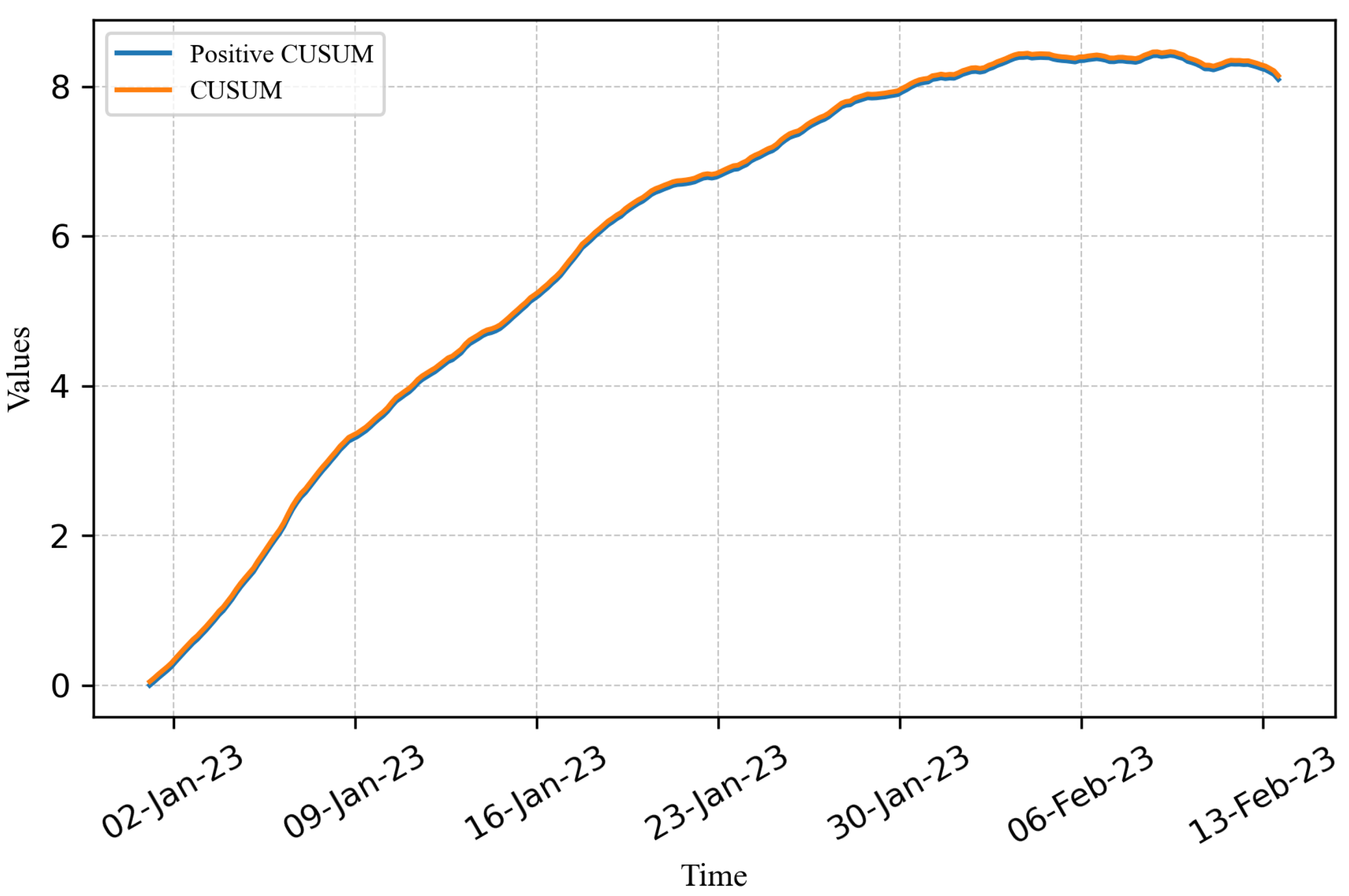
• Calculate the Positive CUSUM value following the steps outlined in Section 5. Subsequently, create a graph that illustrates the Positive CUSUM of the NEI values, plotted against the CUSUM values from January to February, as depicted in Figure 4. It can be seen that if the accumulated changes occur in a positive direction, the Positive CUSUM value will be equal to the CUSUM. This is because the monitoring of fault severity in the transformer focuses only on increasing severity. Decreasing changes are not within the scope of interest. The Positive CUSUM value differs from the CUSUM value when the cumulative sum of the Diff values is negative.
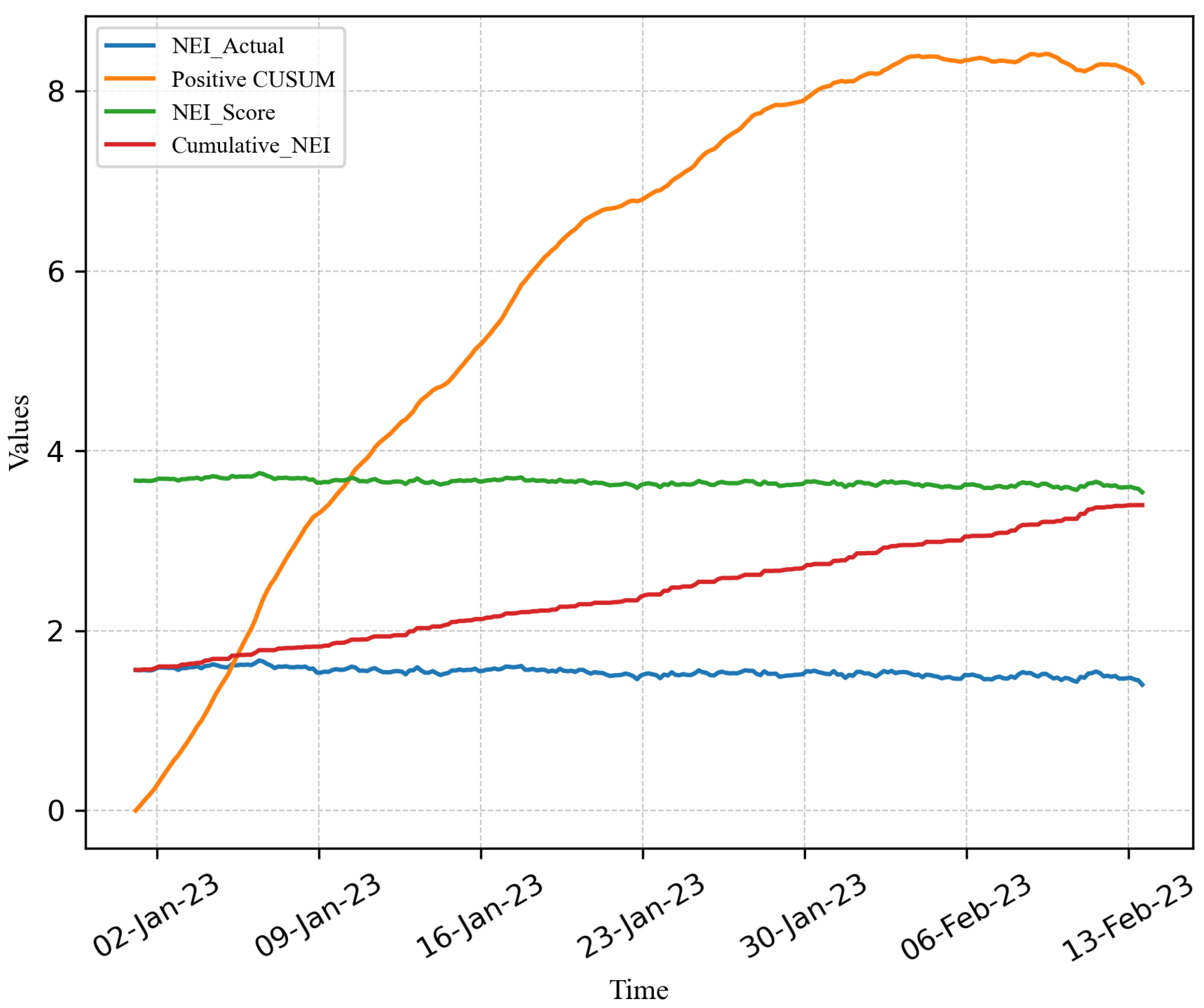
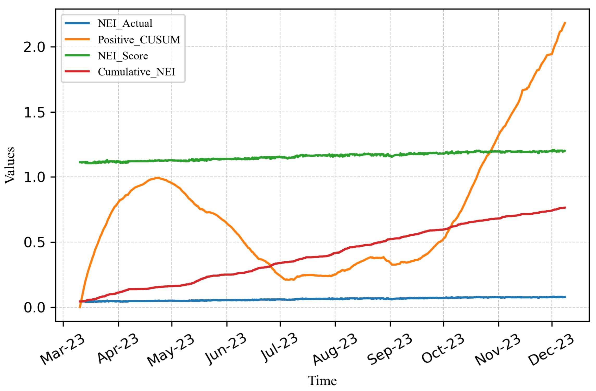
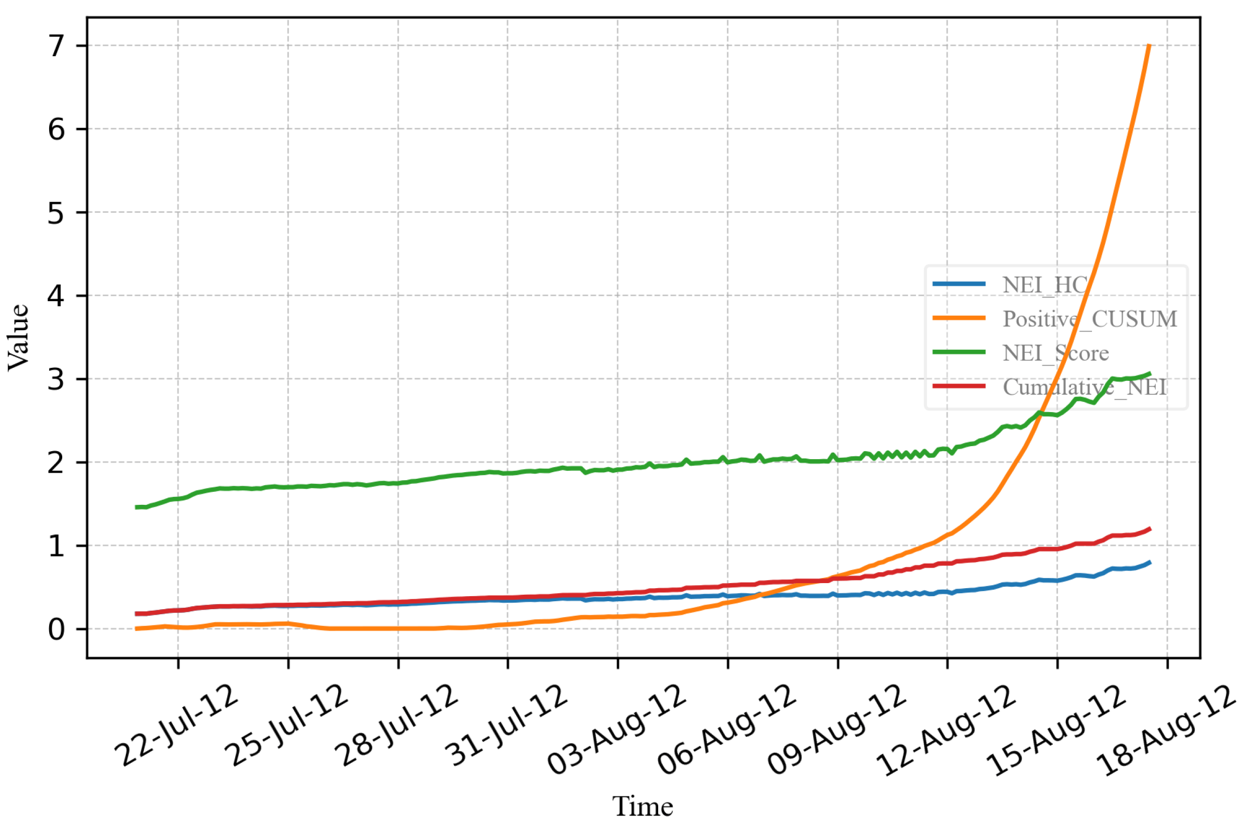
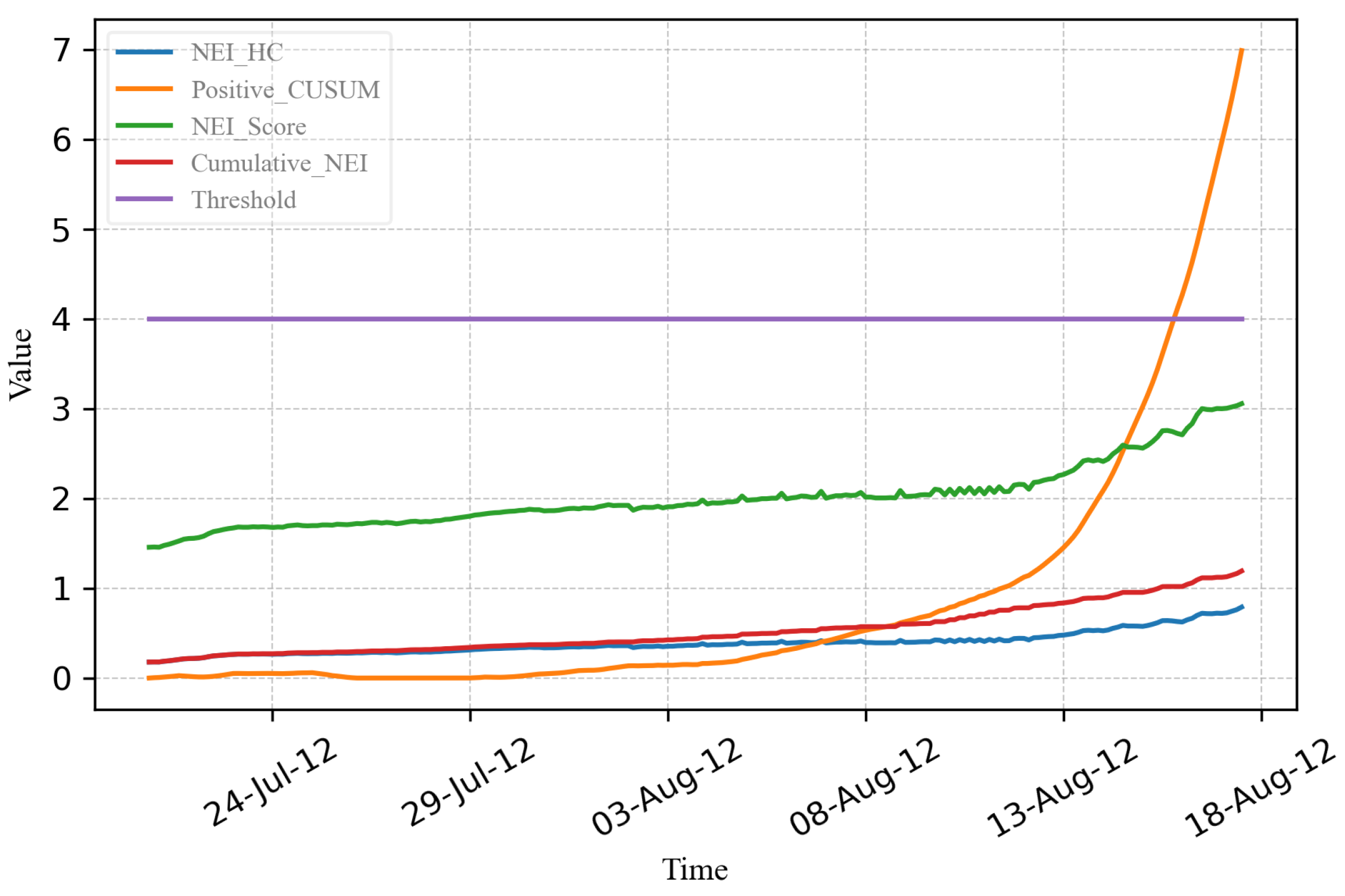
• Create a plot that compares the values of ${\mathrm{NEI}}_{\mathrm{HC}}$ with the Positive CUSUM, NEI score and cumulative NEI, as depicted in Figure 5.

As observed from Figure 5, the Positive CUSUM of NEI exhibits a continuous upward trajectory, reaching a stable value of approximately eight at the end of the data series. Conversely, the cumulative NEI exhibits a steady increase, while both NEI and the NEI score remain relatively constant.

Evaluate the NEI of hydrocarbon gas from March to December

• Determine the correlation between the log(TDCG) and the ${\mathrm{NEI}}_{\mathrm{HC}}$ using linear regression to calculate the coefficient of determination (${\mathrm{R}}^2$) for each month, as illustrated in Table 4. It was discovered that July had the highest ${\mathrm{R}}^2$ value of 0.8532. The linear equation derived from the linear regression, presented in Figure 6, is

  $$NE{I}_{Predict}=1.4306\times log\left(TDCG\right)-2.4192$$

  (10)
• Determine the difference (Diff) between the NEI data obtained from DGA and the NEI calculated using the baseline equation.
• Calculate the Positive CUSUM following the steps outlined in Section 5. Subsequently, create a plot that compares the values of ${\mathrm{NEI}}_{\mathrm{HC}}$ with the Positive CUSUM, NEI score and cumulative NEI, as depicted in Figure 7.

Figure 7 illustrates that the actual NEI and NEI score values exhibit relatively constant trends, while the cumulative NEI exhibits a linear increase. The Positive CUSUM initially rises and reaches its minimum value during the baseline month of July. Subsequently, it remains relatively stable from July to September, and from October to December, the Positive CUSUM continues to increase linearly. This pattern is attributed to the cumulative discrepancy between the actual NEI and the NEI derived from the equation in the baseline month, as shown in Figure 8. The Positive CUSUM clearly shows changes even when there are only slight variations in the NEI levels.

4.

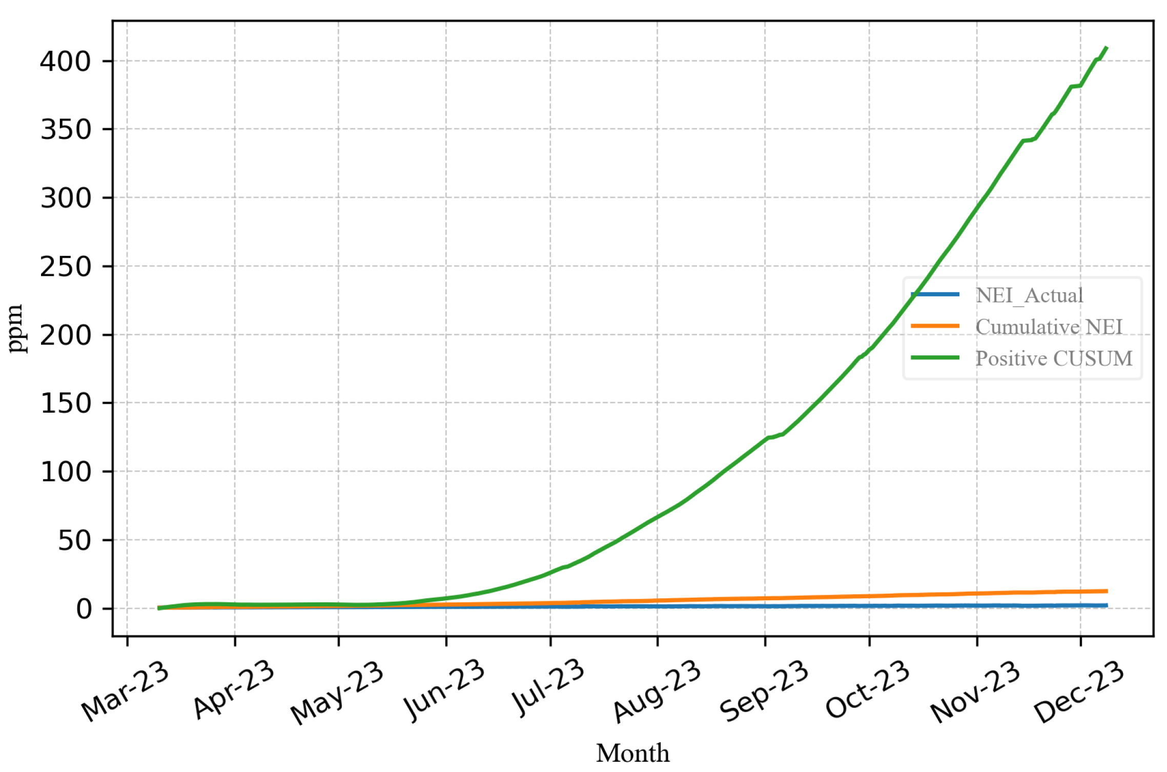
ANOVA tests of Positive CUSUM, NEI, NEI score, and cumulative NEI revealed an F-statistic of 5153.77 and a p-value of 0.0, indicating a significant difference among the four groups (p-value < 0.05), as demonstrated in the boxplot in Figure 9.

Evaluate the NEI of Carbon Oxide Gas from March to December

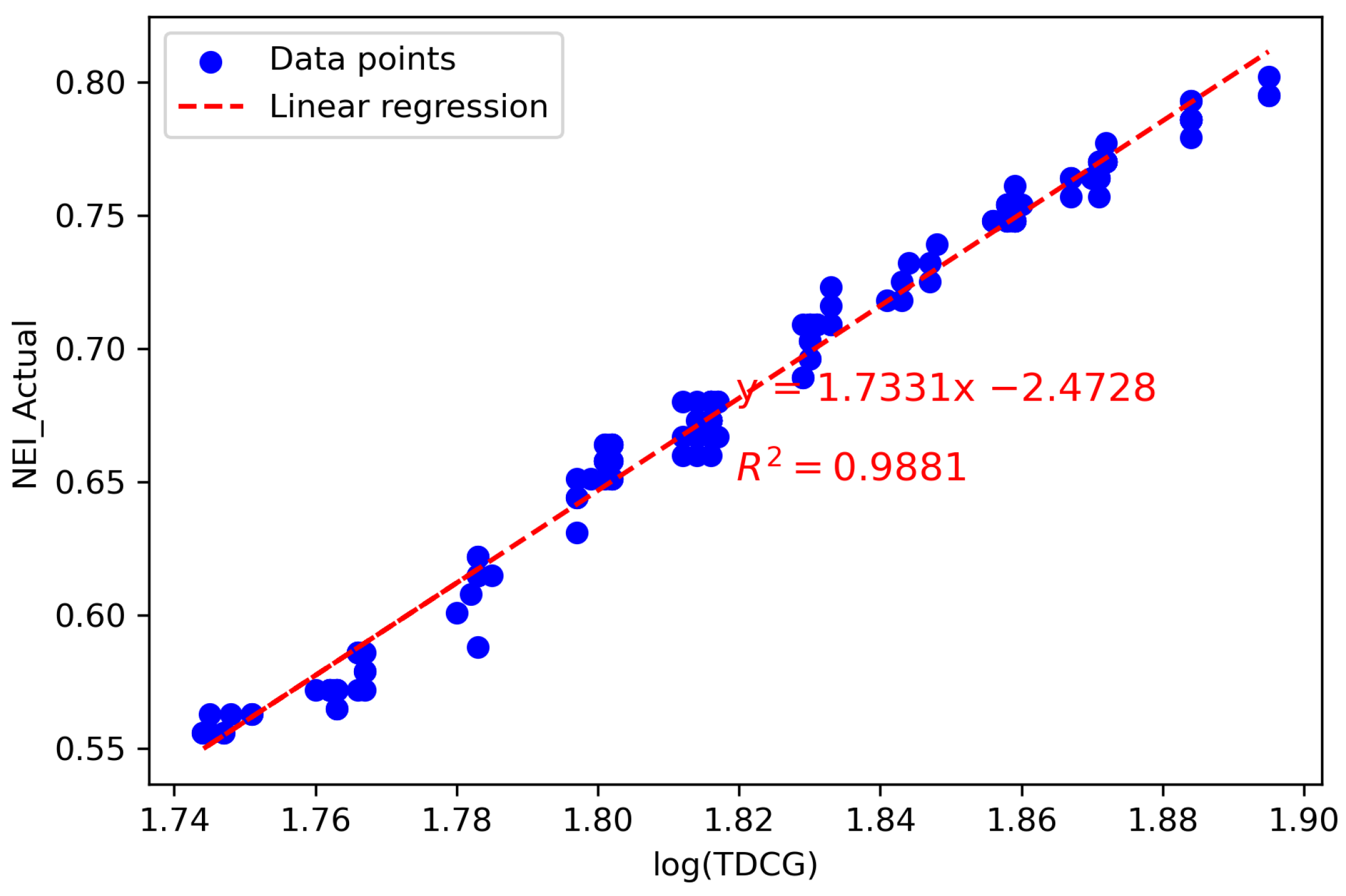
• Employ linear regression analysis to establish a correlation between the logarithm of TDCG and ${\mathrm{NEI}}_{\mathrm{CO}}$. Subsequently, determine the coefficient of determination (${\mathrm{R}}^2$) for each month, as presented in

  Table 5. The correlation coefficient of Carbon Oxide gas from January to December 2023.

  January	February	March	April	May	June
  0.1588	0.9222	0.9072	0.9881	0.9639	0.9726
  July	August	September	October	November	December
  0.9703	0.9404	0.8966	0.9258	0.8026	0.8746

  . The analysis revealed that April exhibited the highest ${\mathrm{R}}^2$ value of 0.9881. The linear regression equation derived from this analysis, depicted in Figure 10, is as follows:

  $$NE{I}_{Predict}=1.7331\times log\left(TDCG\right)-2.4728$$

  (11)
• Calculate the difference (Diff) between the NEI data obtained from the DGA results and the NEI data calculated using the baseline equation.
• Calculate the Positive CUSUM values as per the procedures outlined in Section 5. Subsequently, create a plot that copares the values of the Positive CUSUM of ${\mathrm{NEI}}_{\mathrm{CO}}$ in comparison to the ${\mathrm{NEI}}_{\mathrm{CO}}$ and Cumulative NEI values obtained from March to December, as depicted in Figure 11.

Figure 11 illustrates that the Positive CUSUM values for cellulose insulation exhibit a continuous upward trend, rendering it unsuitable for monitoring the severity of faults related to cellulose insulation. This trend is also evident in the Cumulative NEI presented in Figure 12. As per IEEE C57.104-2019 Annex F [10], the ${\mathrm{CO}}_2/\mathrm{CO}$ ratio is directly proportional to faults associated with cellulose insulation.

4.

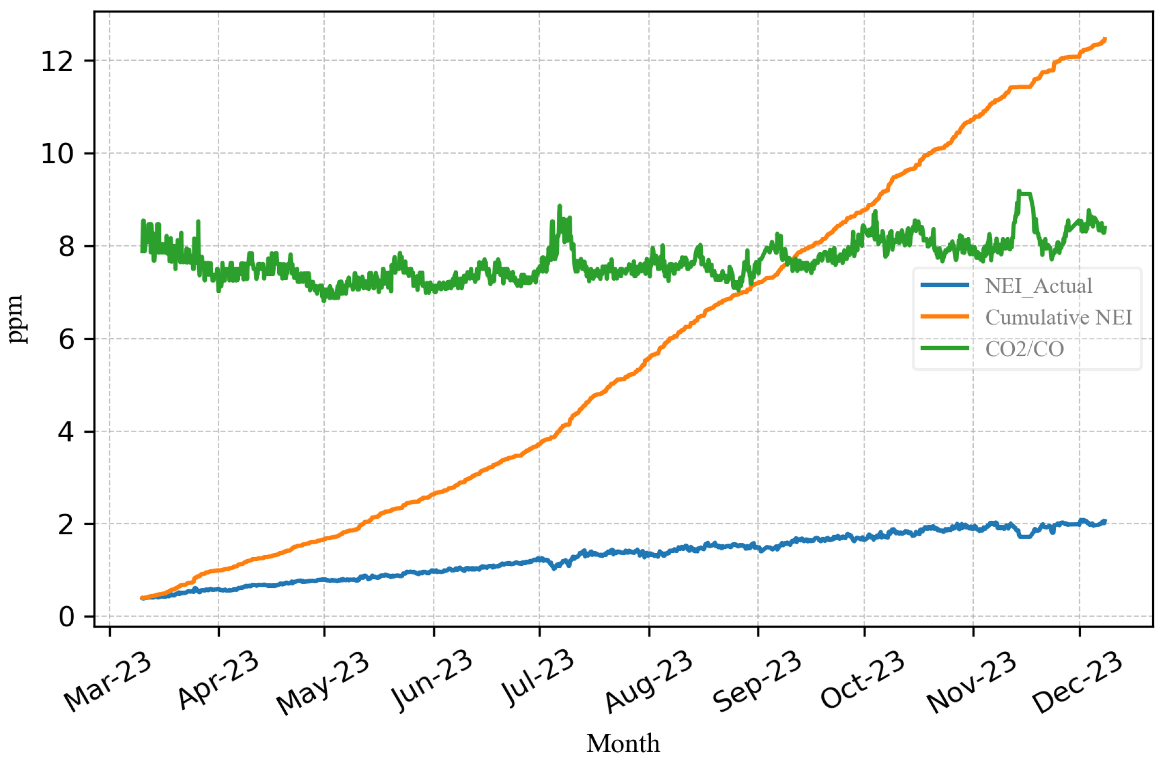
Figure 12 presents a graphical representation of the NEI values in relation to the cumulative NEI and the ${\mathrm{CO}}_2/\mathrm{CO}$ ratio. When a fault occurs in cellulose insulation, the ${\mathrm{NEI}}_{\mathrm{CO}}$ value and the ${\mathrm{CO}}_2/\mathrm{CO}$ ratio are used to track the severity of the fault.

6.2. Transformer in the Steel Industry 2

The steel factory employs a 96 MVA Arc Furnace transformer manufactured in 1992 with a rated voltage of 22/1.1 kV. This transformer is equipped with an online DGA monitoring device from Morgan Schaffer, Model Calisto 9, installed on 31 May 2012, as shown in Figure 13. The device records gas concentration data every three hours. Sample data from 31 May 2012, to 17 August 2012, are presented in

Table 6. Sample DGA results from the steel factory in Case Study 2.

Time	${\mathbf{H}}_2$ (ppm)	${\mathbf{CH}}_4$ (ppm)	${\mathbf{C}}_2{\mathbf{H}}_6$ (ppm)	${\mathbf{C}}_2{\mathbf{H}}_4$ (ppm)	${\mathbf{C}}_2{\mathbf{H}}_2$ (ppm)	$\mathbf{CO}$ (ppm)	${\mathbf{CO}}_2$ (ppm)	${\mathbf{O}}_2$ (ppm)	${\mathbf{N}}_2$ (ppm)	TDCG (ppm)
31 May 2012 04:22	99	91.8	50	64.2	1.6	440	3240	31,200	63,000	746.6
31 May 2012 07:22	104	96.6	51.4	66.6	1.6	445	3350	31,400	65,000	765.2
31 May 2012 10:22	107	99.6	52.6	68.2	1.6	450	3400	31,500	65000	779
31 May 2012 13:22	108	100	52.8	68.4	1.6	460	3450	32,000	66,000	790.8
31 May 2012 16:22	107	101	53.2	69	1.6	455	3450	31,300	66,000	786.8
31 May 2012 19:22	108	100	53.2	68.8	1.6	450	3460	32,300	66,000	781.6
31 May 2012 22:22	108	101	53	68.8	1.6	455	3470	32,300	66,000	787.4

, accompanied by graphs illustrating gas concentration, as depicted in Figure 14.

On 18 July 2012, the transformer underwent maintenance and oil filtration. It was subsequently restored on 20 July 2012. On 12 August 2012, there was an abrupt increase in the transformer’s gas levels, which comprised hydrogen, methane, ethane, and ethylene, as shown in Figure 15. Consequently, the factory removed the transformer from the system for inspection on 23 August 2012.

Use the DGA data collected from the online monitoring device in the following manner:

• Using data from May to August 2012, eliminate any incomplete entries from the DGA results for all nine gas types, sampled every three hours.
• Determine the total dissolved combustible gas (TDCG) and calculate its logarithmic value.
• Determine the values of ${\mathrm{NEI}}_{\mathrm{HC}}$ and ${\mathrm{NEI}}_{\mathrm{CO}}$.
• The information gathered from step 3 will be segmented into monthly data.

Evaluate the NEI of hydrocarbon gas

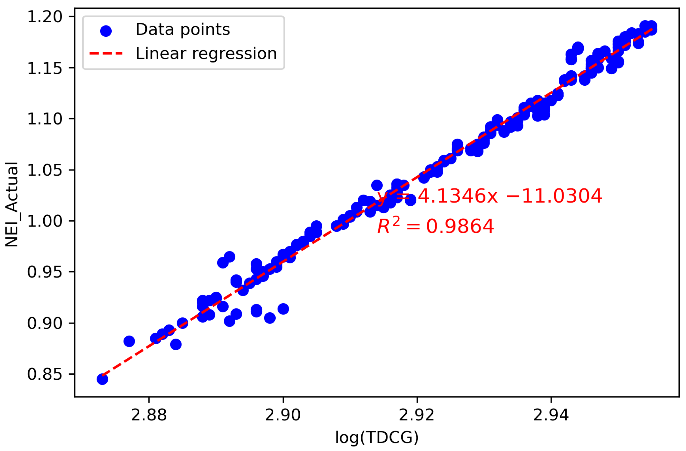
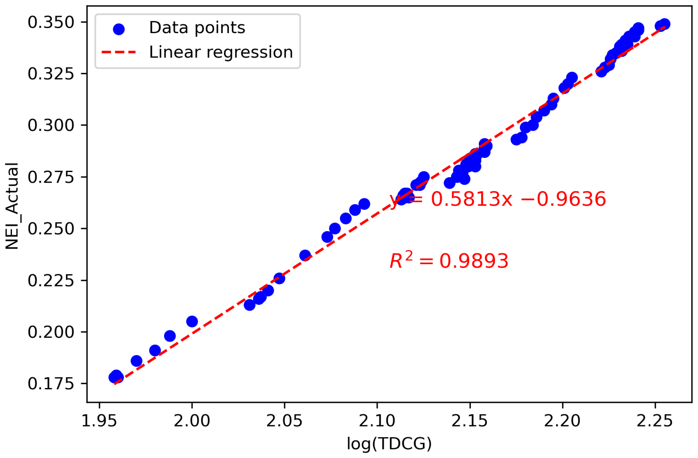
• Determine the correlation between the log(TDCG) and the ${\mathrm{NEI}}_{\mathrm{HC}}$ using linear regression to calculate the coefficient of determination (${\mathrm{R}}^2$) for each month, as illustrated in

  Table 7. Coefficient of determination (${\mathrm{R}}^2$) in Case Study 2.

  May–June	Jul_Pre_Oil Pure.	Jul_Post_Oil Pure.	August
  0.9864	0.9145	0.9893	0.9574

  . It is observed that the highest ${\mathrm{R}}^2$ value before oil purification is 0.9867, and after oil purification, it is 0.9893. The linear equation derived from the linear regression before oil purification, presented in Figure 16, is

  $$\begin{array}{c}\hfill NE{I}_{Predict}=4.1346\times log\left(TDCG\right)-11.03\end{array}$$
  The linear regression after oil purification, presented in Figure 17, is

  $$\begin{array}{c}\hfill NE{I}_{Predict}=0.5813\times log\left(TDCG\right)-0.9636\end{array}$$
• Determine the difference (Diff) between the NEI data obtained from the DGA results and the NEI data calculated using the baseline equation.
• Calculate the Positive CUSUM value following the steps outlined in Section 5. Subsequently, create a graph that compares the values of ${\mathrm{NEI}}_{\mathrm{HC}}$ with the Positive CUSUM, NEI score, and cumulative NEI before and after oil purification, as depicted in Figure 18 and Figure 19.

Figure 18 shows that before transformer maintenance, the Positive CUSUM value was low, while the ${\mathrm{NEI}}_{\mathrm{HC}}$, NEI score, and cumulative NEI gradually increased slightly.

Figure 19 illustrates the monitored values following transformer maintenance. The ${\mathrm{NEI}}_{\mathrm{HC}}$ and cumulative NEI values remained consistently around 1, while the NEI score exhibited a gradual increase from 2 to 3 between 12 August and 18 August 2012. During 12 August to 15 August, the Positive CUSUM value surged from 1 to 3, followed by a rapid increase from 3 to exceeding 7 between 15 August and 18 August. This surge prompted the plant to halt the transformer for inspection.

Evaluate the NEI of Carbon Oxide Gas

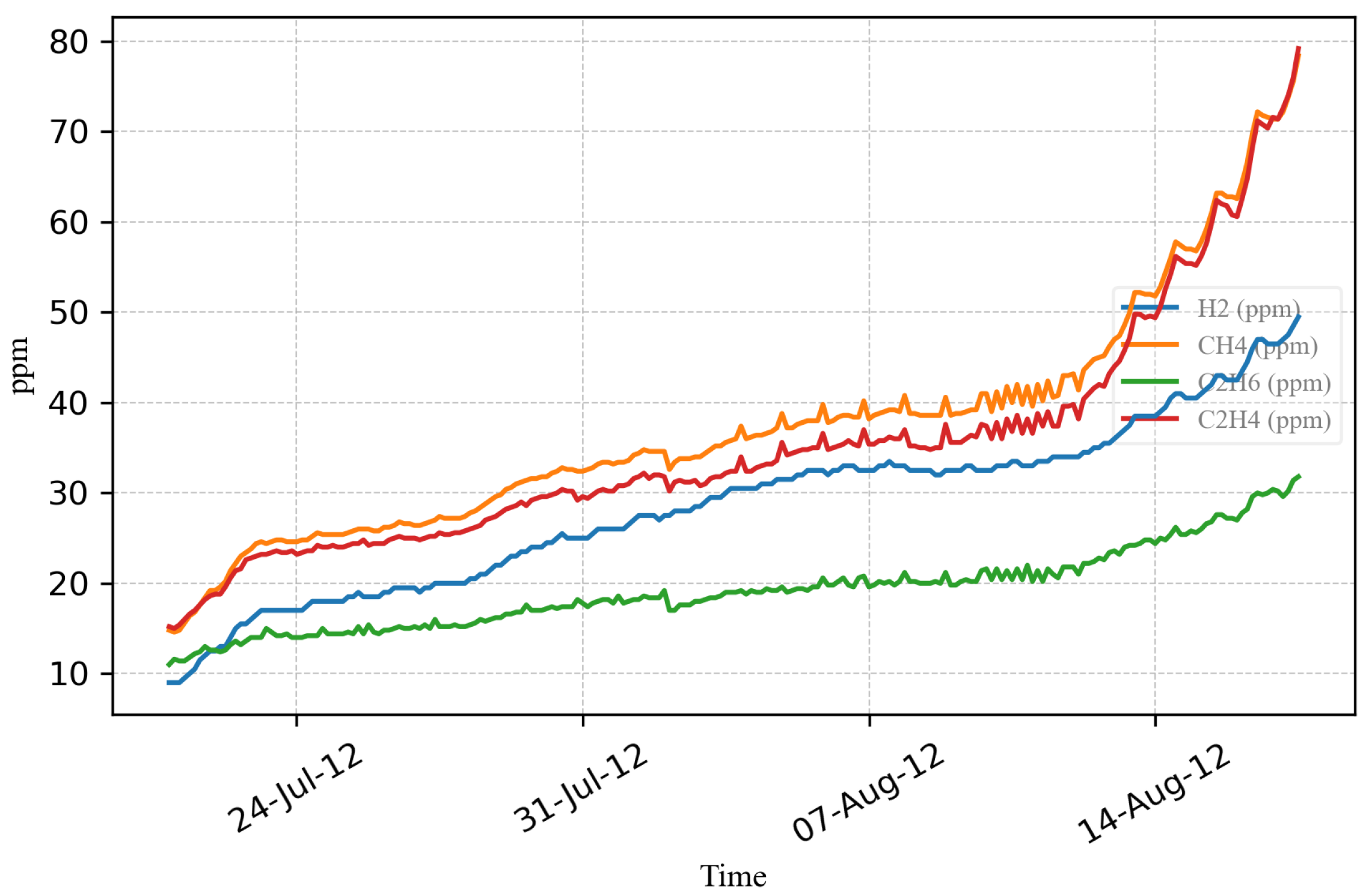
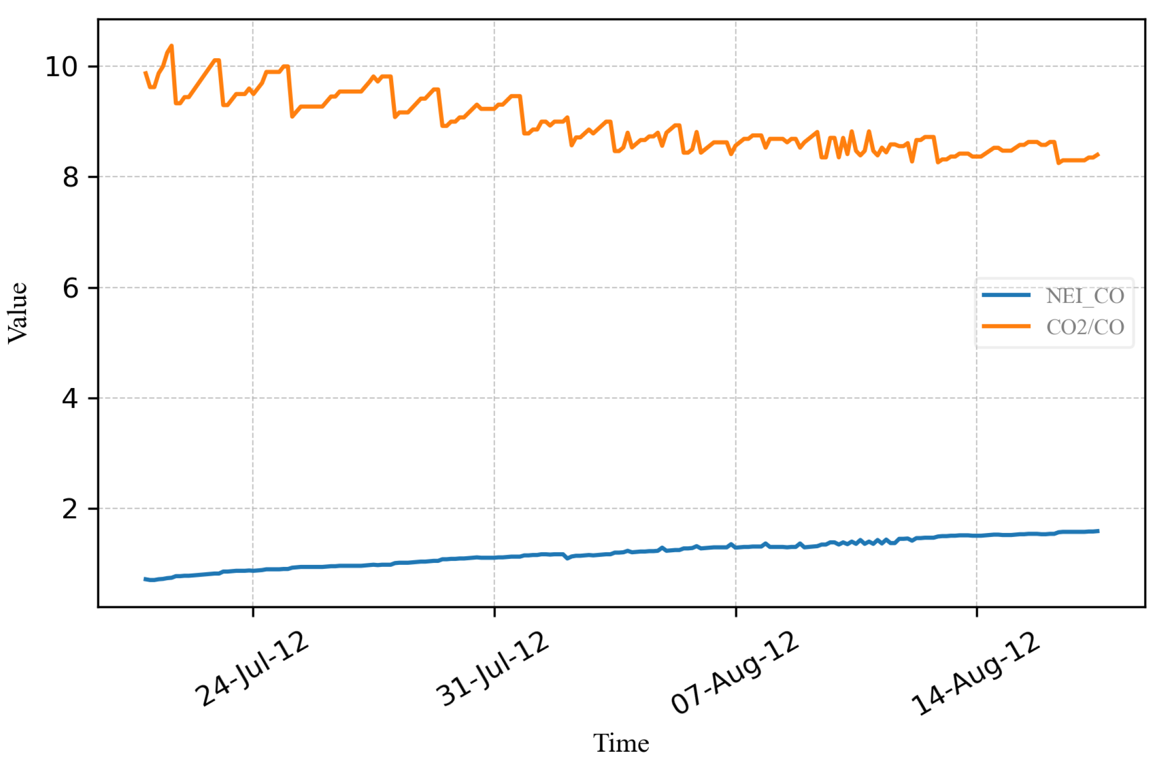
• Figure 20 depicts an ${\mathrm{NEI}}_{\mathrm{CO}}$ graph and the ${\mathrm{CO}}_2/\mathrm{CO}$ ratio prior to the transformer’s maintenance and oil filtration. Both the ${\mathrm{NEI}}_{\mathrm{CO}}$ graph and the ${\mathrm{CO}}_2/\mathrm{CO}$ ratio exhibit relatively stable behavior.
• Figure 21 presents the graph of ${\mathrm{NEI}}_{\mathrm{CO}}$ and the ${\mathrm{CO}}_2$/CO ratio after maintenance and filtration of the transformer oil. It was observed that the ${\mathrm{NEI}}_{\mathrm{CO}}$ value exhibited a substantial decrease, while the ${\mathrm{CO}}_2$/CO ratio experienced a modest increase.

The results suggest that the fault is not related to the cellulose insulation.

Following the opening of the transformer for internal inspection, the cause of the abnormality was identified as a burnt connection between phase A and phase B, as illustrated in Figure 22 and Figure 23.

The decision threshold for Positive CUSUM, which serves as an indicator of abnormal events within the transformer, was determined with reference to the NEI score. Specifically, a threshold value of 4 was adopted, as illustrated in Figure 24. As shown in Figure 24, the Positive CUSUM value surpassed this threshold at 20:57 on 15 August 2012.

7. Conclusions

This research article analyzes fault severity in transformers using dissolved gas analysis of transformer oil, employing the Positive CUSUM method from NEI. It evaluates fault severity in transformers through case studies involving online DGA results from arc furnace transformers at two steel plants. These case studies compare the results with NEI, NEI score, and cumulative NEI. This study found that the Positive CUSUM method provides more evident trends in assessing fault severity from hydrocarbon gas compared to NEI, NEI score, and cumulative NEI. In contrast, using NEI values derived from carbon oxide gas, along with the $\mathrm{C}{\mathrm{O}}_2/\mathrm{C}\mathrm{O}$ ratio specified in Annex F of IEEE C57.104-2019 [10], yields better results in evaluating the severity trends of faults related to cellulose insulation.

Because of the widespread acceptance of using DGA to assess the condition of insulation within transformers, making it an important topic within power transformers, there has been increasing installation of online DGA monitors for critical power transformers in production processes at factories. A further research study to further develop the Positive CUSUM method will integrate artificial intelligence (AI) with various optimization techniques to identify optimal parameters [27,28,29,30,31]. Consequently, in the future, when combining this AI-enhanced Positive CUSUM method with online DGA data sources to monitor the severity trends of internal transformer faults, there will be an increase in case studies for the analysis and further development of real-time diagnostics for online DGA-monitoring systems.

References

- Grisaru, M. A century of dissolved gas analysis-part II. Transform. Mag. 2019, 6, 90–101. [Google Scholar]
- Apribowo, C.H.B.; Sudjono, A.; Rachmatika, R.; Maghfiroh, H. Designing Automatic Syringe Shaker as The Supporting Media for Method of Dissolved Gas Transformer Oil Analysis. In Proceedings of the 2019 6th International Conference on Electric Vehicular Technology (ICEVT), Bali, Indonesia, 18–21 November 2019; pp. 263–266. [Google Scholar]
- Shutenko, O.; Kulyk, O. Comparative Analysis of the Defect Type Recognition Reliability in High-Voltage Power Transformers Using Different Methods of DGA Results Interpretation. In Proceedings of the 2020 IEEE Problems of Automated Electrodrive, Theory and Practice (PAEP), Kremenchuk, Ukraine, 21–25 September 2020; pp. 263–266. [Google Scholar]
- Taha, I.B.M.; Ghoneim, S.S.M.; Zaini, H.G. Improvement of Rogers four ratios and IEC Code methods for transformer fault diagnosis based on Dissolved Gas Analysis. In Proceedings of the 2015 North American Power Symposium (NAPS), Charlotte, NC, USA, 4–6 October 2015; pp. 1–5. [Google Scholar]
- Leivo, S.; Sattler, D.; Duval, M.; Chiarella, C. A Case Study: Transformer Failure Detected with Real-time DGA Monitoring. In Proceedings of the 2023 IEEE Electrical Insulation Conference (EIC), Quebec City, QC, Canada, 18–22 June 2023; pp. 1–4. [Google Scholar]
- Mawelela, T.U.; Nnachi, A.F.; Akumu, A.O.; Abe, B.T. Fault Diagnosis of Power Transformers Using Duval Triangle. In Proceedings of the 2020 IEEE PES/IAS PowerAfrica, Nairobi, Kenya, 25–28 August 2020; pp. 1–5. [Google Scholar]
- Duval, M.; dePabla, A. Interpretation of gas-in-oil analysis using new IEC publication 60599 and IEC TC 10 databases. IEEE Electr. Insul. Mag. 2001, 17, 3–4. [Google Scholar] [CrossRef]
- Guardado, J.L.; Naredo, J.L.; Moreno, P.; Fuerte, C.R. A comparative study of neural network efficiency in power transformers diagnosis using dissolved gas analysis. IEEE Trans. Power Deliv. 2001, 16, 643–647. [Google Scholar] [CrossRef]
- IEC 60599:2015; Interpretation of the Analysis of Gases in Transformers and Other Oil-Filled Electrical Equipment in Service. IEC: Geneva, Switzerland, 2015.
- IEEE Std C57.104-2019; IEEE Guide for the Interpretation of Gases Generated in Mineral Oil-Immersed Transformers. IEEE: New York, NY, USA, 2019.
- Jakob, F.; Noble, P.; Dukarm, J.J. A Thermodynamic Approach to Evaluation of the Severity of Transformer Faults. IEEE Trans. Power Deliv. 2012, 27, 554–559. [Google Scholar] [CrossRef]
- Jakob, F.; Dukarm, J.J. Thermodynamic Estimation of Transformer Fault Severity. IEEE Trans. Power Deliv. 2015, 30, 1941–1948. [Google Scholar] [CrossRef]
- Cruz, V.G.M.; Costa, A.L.H.; Paredes, M.L.L. Development and evaluation of a new DGA diagnostic method based on thermodynamics fundamentals. IEEE Trans. Dielectr. Electr. Insul. 2015, 22, 888–894. [Google Scholar] [CrossRef]
- Irungu, G.K.; Akumu, A.O.; Munda, J.L. Application of dissolved gas analysis in maintenance ranking of faulty oil-filled electrical equipment based on type and energy of the fault. In Proceedings of the 2017 IEEE Electrical Insulation Conference (EIC), Baltimore, MD, USA, 11–14 June 2017; pp. 274–278. [Google Scholar]
- Dukarm, J.J.; Duval, M. Transformer Reliability and Dissolved-Gas Analysis. In Proceedings of the 2016 Cigre Canada Conference, Vancouver, BC, Canada, 17–19 October 2016; pp. 1–8. [Google Scholar]
- Guo, R.; Wang, J.; Liu, R.; Ping, A.; Xiao, R.; Wang, J. An Improved Method to Evaluate the Severity of Discharges with DGA Based on Thermodynamics. In Proceedings of the 2021 International Conference on Electrical Materials and Power Equipment (ICEMPE), Chongqing, China, 11–15 April 2021; pp. 1–4. [Google Scholar]
- Dukarm, J.J.; Draper, Z.H. Dissolved-Gas Analysis for Nitrogen-Blanketed Transformers. In Proceedings of the 2020 IEEE PES Transmission and Distribution Conference and Exhibition-Latin America (T&D LA), Montevideo, Uruguay,, 28 September–2 October 2020; pp. 1–5. [Google Scholar]
- Ali, S.; Shah, I.; Wang, L.; Yue, Z. A Comparison of Shewhart-Type Time-Between-Events Control Charts Based on the Renewal Process. IEEE Access 2020, 8, 113683–113701. [Google Scholar] [CrossRef]
- Xia, X.; Lin, J.; Xiao, Y.; Cui, J.; Peng, Y.; Ma, Y. A Control-Chart-Based Detector for Small-Amount Electricity Theft (SET) Attack in Smart Grids. IEEE Internet Things J. 2022, 9, 6745–6762. [Google Scholar] [CrossRef]
- Tabella, G.; Ciuonzo, D.; Paltrinieri, N.; Rossi, P.S. Bayesian Fault Detection and Localization Through Wireless Sensor Networks in Industrial Plants. IEEE Internet Things J. 2024, 11, 13231–13246. [Google Scholar] [CrossRef]
- Venkatesulu, G.; Akhtar, P.M.; Sainath, B.; Murthy, B.R.N. Continuous Acceptance Sampling Plans for Truncated Lomax Distribution Based on CUSUM Schemes. Int. J. Math. Trends Technol. 2018, 55, 174–184. [Google Scholar]
- Tyagi, D.; Yadav, V. Combined Quality Control Scheme for Monitoring Autocorrelated Process. Thai Stat. 2024, 22, 986–1005. [Google Scholar]
- Vargas, V.C.C.; Lopes, L.F.D.; Souza, A.M. Comparative study of the performance of the CUSUM and EWMA control charts. Comput. Ind. Eng. 2004, 46, 707–724. [Google Scholar] [CrossRef]
- Puranik, V.S. CUSUM quality control chart for monitoring energy use performance. In Proceedings of the 2007 IEEE International Conference on Industrial Engineering and Engineering Management, Singapore, 2–5 December 2007; pp. 1231–1235. [Google Scholar]
- Ratsame, P.; Chansri, P. Analysis of Electrical Energy Consumption Efficiency Trends Using Visualization Tools. In Proceedings of the 2024 8th International Conference on Power Energy Systems and Applications (ICoPESA), Hong Kong,, 15–17 January 2024; pp. 333–337. [Google Scholar]
- Siebert, L.C.; Yamakawa, E.K.; Aoki, A.R.; Ferreira, L.R. Energy efficiency indicators assessment tool for the industry sector. In Proceedings of the 2014 IEEE PES Transmission & Distribution Conference and Exposition-Latin America (PES T&D-LA), Medellin, Colombia, 10–13 September 2014; pp. 1–6. [Google Scholar]
- Tao, L.; Yang, X.; Zhou, Y.; Yang, L. A Novel Transformers Fault Diagnosis Method Based on Probabilistic Neural Network and Bio-Inspired Optimizer. Sensors 2021, 21, 3623. [Google Scholar] [CrossRef] [PubMed]
- Wang, L.Z.; Chi, J.F.; Ding, Y.Q.; Yao, H.-Y.; Guo, Q.; Yang, H.-Q. Transformer fault diagnosis method based on SMOTE and NGO-GBDT. Sci. Rep. 2022, 14, 7179. [Google Scholar] [CrossRef] [PubMed]
- Liu, C.; Yang, W. Transformer fault diagnosis using machine learning: A method combining SHAP feature selection and intelligent optimization of LGBM. Energy Inform. 2025, 8, 52. [Google Scholar] [CrossRef]
- Kesphrom, N.; Nedphokaew, S.; Ruangsap, N.; Rugthaicharoencheep, N. Power Distribution System Improvement Planning Considering Financial Losses Due to Faults in Power Systems. Energies 2025, 18, 938. [Google Scholar] [CrossRef]
- Rokani, V.; Kaminaris, S.D.; Karaisas, P.; Kaminaris, D. Power Transformer Fault Diagnosis Using Neural Network Optimization Techniques. Mathematics 2023, 11, 4693. [Google Scholar] [CrossRef]