Abstract
In this study, a Long Short-Term Memory (LSTM) model with extra variables such as weather conditions and school days was developed within a multi-scale framework in order to forecast passenger flow in both bus and rail systems, covering both regional and route-level analyses. In addition, the performance of the LSTM model was compared against three separate deep learning models. Among these, the Nonlinear Autoregressive Network with Exogenous Inputs (NARX) time series model produced the lowest error values, achieving a high level of accuracy. While no considerable changes were observed in regional rail passenger flow as a result of the inclusion of weather-related variables, a 2.2% drop in the RMSE value was achieved in bus passenger flow at the regional level; however, this improvement remains relatively modest. In contrast, at the route level, RMSE values declined by 2.4% for rail and 3.69% for bus routes. These findings reveal that the inclusion of weather-related variables significantly improves the prediction of bus passenger flow, underlining the benefits of integrating such data into forecasting models. Furthermore, the findings of this study analytically support transportation planners in making more informed, data-driven decisions regarding scheduling and capacity management.
1. Introduction
In the recent past, increasing population density and urbanization in large cities have led to the concentration of business centers in certain areas, putting considerable pressure on transportation infrastructure. This strain adversely impacts the efficiency of public transportation systems, adds to increased traffic congestion, and causes extended travel times. Delays in public transport, in particular, encourage individuals to use private vehicles, thereby aggravating carbon emissions and contributing to environmental pollution []. The increase in traffic density directly affects the performance of public transport modes such as bus services []. Delays and irregular passenger volumes undermine public confidence in transportation services and, therefore, necessitate developing strategies aimed at enhancing service quality for a more sustainable and environmentally friendly system. Since bus and subway systems, compared to private vehicles, generate significantly markedly diminished greenhouse gas output, both short- and long-term passenger flow forecasts are crucial for the sustainability of public transportation. While long-term forecasts generally demonstrate consistent trends, short-term predictions are prone to sudden fluctuations caused by factors such as weather conditions, cultural events, or sporting activities that can lead to congestion and increased travel times. In light of the recent concept of “Smart Mobility”, all transportation systems aim to integrate with each other via information and communication technologies. As such, intelligent transportation systems (ITSs) are becoming increasingly important. For public transportation services—a key component of intelligent transportation systems—to operate more consistently, it is crucial to design them accurately, with the projection of future passenger demand forming a fundamental part of this process. Moreover, long-term forecasts are valuable for urban planning and policy-making; however, short-term predictions require real-time and up-to-date data for operational decisions [].
Given the possibility of unexpected passenger surges at particular times of the day, it becomes imperative to adjust transit schedules accordingly. Collecting relevant data was once a significant challenge, but the emergence of Advanced Public Transportation Systems (APTSs) has greatly simplified the process. Technologies such as Automatic Vehicle Location (AVL) and Automatic Passenger Counting (APC), which are integral to APTSs, now enable the real-time collection of operational data []. The integration of these data sources notably enhances the accuracy of short-term forecasts, offering significant benefits to local authorities and urban planners in managing passenger demand, improving travel comfort, and decreasing operational costs []. Therefore, passenger flow forecasting has a critical role in intelligent transportation systems [].
2. Literature Review
As passenger demand forecasting, by nature, focuses on predicting the number of passengers within a given time interval and should thus be assessed within the context of a time series analysis. However, because of the complex and nonlinear relationships in a time series, traditional statistical techniques can often fall short [].
Various statistical and machine learning approaches have been employed in previous studies to forecast passenger volumes, including regression analysis [], Support Vector Machines (SVMs) [], Artificial Neural Networks (ANNs) [], Bayesian models [], and Gradient Boosting techniques []. Several researchers focusing on short-term forecasting have contributed insights into passenger flow prediction using diverse methodologies.
One of the earliest studies adopting a statistical approach was by Ahmed and Cook, who employed the AutoRegressive Integrated Moving Average (ARIMA) model to predict highway traffic flow []. Among time series models, ARIMA and its variants are widely used. Williams et al. developed the Seasonal ARIMA (SARIMA) model by incorporating seasonal components in traffic data []. Similarly, Ye et al. utilized a three-month dataset to predict daily bus passenger flow and analyzed the performance of the model by combining weekday and weekend data []. However, in many cases, such statistical models often yield high error rates, particularly in nonlinear passenger flows with heavy irregular fluctuations [].
Thus, to reduce error rates and achieve better forecast accuracy, Kalman filtering techniques were also wisely used alongside ARIMA models, eliminating the noisy data []. Jiao et al. further developed the Kalman filtering model by integrating it with the Bayesian method to better predict rail passenger flow []. In another study, time series data from train stations were analyzed using Facebook’s Prophet model, demonstrating superior performance over ARIMA in certain contexts []. The limitations of linear models—especially when ample training data are available—have led to the adoption of machine learning (ML) approaches []. Liu and Yao developed a revised model based on the Least Squares Support Vector Machines (LSSVM) model to forecast passenger density in metro stations in Guangzhou [].
In addition to traditional ML methods, deep learning (DL) models offer significant advantages in understanding nonlinear structures [,]. In particular, DL models yield more successful results in forecasting both forward and backward time series features []. DL models are known for their powerful computational capabilities and are more skilled at managing complicated functions compared to standard machine learning algorithms []. By utilizing multilayer network architectures and non-sequential optimization techniques that do not follow a regular order, DL models can autonomously filter out meaningful features from data at diverse abstraction levels []. Deep learning models have demonstrated high levels of success not only in forecasting tasks but also in complex classification problems such as image recognition. This highlights their robustness and reliability across different data domains []. Convolutional Neural Networks (CNNs) and Recurrent Neural Networks (RNNs), two fundamental tools of deep learning methods, exhibit high performance in catching spatial dependencies []. RNN models deal with input sequences step by step in temporal order, maintaining a state vector at each step that represents the temporal dynamics of past information within the hidden layers. In comparison to traditional models such as ANNs and CNNs, this network architecture is particularly sensitive to short-term dependencies owing to its memory-based mechanism. However, it may face limitations in modeling long-term dependencies []. To address difficulties such as information loss and gradient vanishing commonly encountered in classical RNNs, LSTM networks were developed. Compared to traditional deep learning models such as ANNs, CNNs, and RNNs, Long Short-Term Memory (LSTM) networks have demonstrated superior performance, particularly in sequential datasets like time series, due to their ability to capture long-term dependencies more effectively []. For instance, a study demonstrated that, compared to RNN, which was limited by vanishing gradient issues, and SVR, which exhibited overgeneralization, the LSTM model yielded superior predictive accuracy across all evaluated performance metrics [].
LSTM networks are more adept at learning long-term dependencies and have been shown to surpass models like ARIMA, SARIMA, and Space-Time ARIMA (STARIMA) in studies performed on metro systems []. Halyal et al. revealed that the LSTM model represents stochastic and nonlinear structures more effectively than the SARIMA model in their study utilizing APC data []. In addition, in a study utilizing smartcard data for passenger flow forecasting, the LSTM model was compared with traditional models such as MLP, SVM, and RBF, and was shown to outperform them in terms of prediction accuracy [].
In recent years, LSTM models have been widely adopted for passenger flow forecasting due to their capability to capture sudden fluctuations and elaborate patterns in time series data []. As a result, deep learning models have gained broad application in time series forecasting. For instance, Zhang et al. employed the LSTM model for short-term passenger flow prediction in rail systems, underlining its faster convergence and greater stability [,]. Similarly, Shao and Soong reported that a station-based LSTM time series model was capable of effectively capturing nonlinear dynamics in passenger flow forecasting []. Hao et al. further integrated two exogenous factors—weekdays and weekends—into the LSTM deep learning model and demonstrated that including these variables considerably enhances prediction accuracy []. Moreover, in a comparative analysis of hourly PM2.5 levels using LSTM, GRU, and CNN-LSTM, the LSTM model outperformed the more complex CNN-LSTM structure in terms of prediction accuracy []. Liu et al. demonstrated that the LSTM model outdoes methods such as Random Forest (RF), SVM, K-Nearest Neighbors (KNN), and Gradient Boosting (GB) in a comparative analysis using six years of data from the Wuhan–Guangzhou high-speed railway []. Han et al. further enhanced the LSTM model using Nadam and SGD optimization algorithms, reaching improved results in ridership forecasting [].
Similarly to the LSTM’s capacity to learn long-term dependencies and lessen the vanishing gradient problem, the Gated Recurrent Unit (GRU) model was developed, offering a more simplified architecture []. Some studies have indicated that the GRU is more effective in capturing sudden fluctuations, especially short-term increases and decreases []. A comparative analysis of LSTM, GRU, and RNN for electricity load forecasting found that GRU achieved the best overall performance []. However, other research suggests that the GRU does not hold absolute superiority over the LSTM; rather, it performs better only under specific data structures and scenarios [].
While the simpler structure of the GRU facilitates faster processing, the LSTM, with its greater number of parameters, is better suited for dealing with large-scale and complex problems []. For instance, Shiwakoti et al. (2024) compared these models across various demand patterns—such as weekdays, weekends, and holidays—and found that both architectures effectively adapt to temporal variability, highlighting their practical potential in short-term forecasting applications [].
This study assumes that meteorological conditions may play a significant role in forecasting passenger flow. However, the existing literature provides limited research that directly examines the impact of weather-related variables on ridership in public transportation systems. To address this gap, meteorological data were added to the model as independent variables. Moreover, calendar-based factors such as public holidays and school days, along with temporal features were additionally integrated. Furthermore, the application of the NARX model in short-term passenger demand forecasting is rarely seen in the current literature, indicating a methodological limitation. Another significant shortcoming is the lack of studies that offer a comparative analysis of bus and rail passenger volumes at both regional and route-specific scales. This study aims to contribute to the literature by addressing these theoretical and methodological gaps.
Prior to proceeding to the forecasting modeling, the XGBoost algorithm was employed for feature selection to evaluate the importance of variables and improve the efficiency of the model. Because of its capacity to model dynamic time-related dependencies and take into account both present and historical data, the LSTM network was selected as the main forecasting model in this study. Although numerous deep learning models have been built for forecasting passenger demand in public transportation, choosing the most fitting model for practical use remains a key problem. In this context, four models were compared, and their performances were assessed using the RMSE metric. Additionally, the Friedman test was used to determine the statistical significance of differences between the models, and recommendations for model selection were provided. As part of the application, the study aims to forecast passenger numbers for both bus and rail systems using an LSTM-based deep learning model. Ridership data were sourced from the Istanbul Metropolitan Municipality (IMM) IT Department, while meteorological data were obtained from the Turkish State Meteorological Service (MGM). By analyzing different data sources in a holistic way, the model built with these data seeks to deliver more realistic and reliable forecasts.
This study offers significant advancements through four basic contributions:
- In order to enhance the accuracy of passenger flow forecasting for both bus and rail systems, the model includes not only time-dependent independent variables (hour, day, month, day of the week) but also external factors such as school days, public holidays, and atmospheric variables (temperature, precipitation, humidity, wind speed, cloudiness, and snowfall) that may influence ridership.
- Prior to proceeding with the forecasting models, a feature importance analysis was conducted using the XGBoost algorithm to assess the significance of the independent variables incorporated in the model. This analysis enabled the identification of the most influential variables, and then, the feature selection process was conducted by determining the variables that most affected the efficiency of the model.
- Passenger flow prediction was conducted on both regional and route-specific levels, covering rail and bus lines. Special attention was given to evaluating passenger behavior along routes shared by both modes of transport.
- The prediction process was started with the LSTM model, followed by the application of advanced deep learning algorithms such as GRU, RNN, and NARX. The performance of these models was then evaluated through comparative analysis.
The structure of the rest of this paper is as follows:
Section 2 gives a comprehensive overview of the data utilized, the initial data handling procedures implemented, the evaluation metrics applied, and outlines the main methodological framework.
Section 3 presents the results of the forecasting experiments for bus and rail passenger numbers, including a performance assessment of the models using appropriate error measurement criteria.
Section 4 offers an in-depth discussion of the outcomes, addresses the study’s limitations and the shortcomings of current approaches, and outlines recommendations for future investigations.
Section 5 concludes the study by summarizing the findings, highlighting the role of weather parameters in passenger forecasting, and proposing future directions for achieving more accurate and comprehensive predictions.
3. Materials and Methods
This section details the processes of data gathering, initial data processing, implementation of deep learning techniques, and identification of features related to bus and rail system passenger numbers.
3.1. Parameter Acquisition and Preprocessing
To estimate hourly bus passenger numbers, in addition to temporal data, meteorological data, as well as information concerning public holidays and school days, were used. In DL models, the correct selection of input variables is vital for the model’s success. Hence, to improve the accuracy of passenger number estimations, weather conditions for the corresponding time slots were also included in the analysis, and their effects on bus and rail systems were analyzed. In this study, two different sets of independent variables were generated. The first dataset includes time-based parameters along with public holiday and school day variables. The second dataset contains only meteorological parameters. The dependent variable (output) is the hourly passenger number for buses and rail systems. Passenger count data were retrieved from the Istanbul Metropolitan Municipality database and consist of hourly recorded boarding data throughout the year via smart card systems. The study is restricted to the Asian side of Istanbul; the transportation network map for this region is presented in Figure 1. The initial phase of the study was conducted on a regional scale, calculating the number of passengers using the bus and rail systems across the entire Asian side.
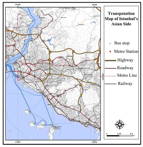
Figure 1.
Asian side of Istanbul bus lines.
In the second phase of the study, conducted on a route-specific level, two rail lines were examined: the Kadıköy–Kartal metro and the Gebze–Üsküdar commuter line. Bus lines operating along the routes of these two rail lines were identified and incorporated into the analysis. Specifically, this approach aimed to enable a relative evaluation of bus lines sharing the same transportation corridor with the rail systems. Figure 2 visualizes the two rail lines in red and black, and the 36 bus lines overlapping with these routes are shown in blue. This map depicts the spatial coverage of the study and the geographical distribution of the transportation lines analyzed.
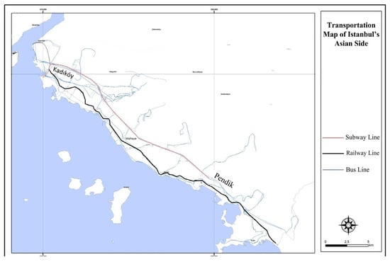
Figure 2.
Subway and bus lines on the Kadıköy–Pendik route.
The second database used in the study comprises hourly meteorological parameters documented between 1 July 2021 and 31 January 2023 by the Turkish State Meteorological Service. This collection contains hourly readings of average temperature (°C), precipitation (mm), humidity (%), wind speed (m/s), cloudiness (okta), and snow depth (cm) for the Asian side. Since the route-specific analysis concentrates on the Kadıköy–Pendik line, two meteorological stations situated along the route—station 17064 (Istanbul–Regional) and station 17813 (Kadıköy–Göztepe)—were included in the study.
Histogram charts displaying the distribution of meteorological data are presented in Figure 3. Temperature ranges approximately between 0 °C and 35 °C, demonstrating a bimodal pattern reflecting seasonal variations. Most precipitation values are near zero. Wind speed displays a right-skewed spread, indicating that lower wind speeds are more widespread. Humidity mirrors a trend close to normal, concentrated between 50% and 80%. For cloudiness, clear skies (0 okta) and complete overcast circumstances (8 okta) are most frequently observed. Snow depth, like rainfall, predominantly hovers near zero.
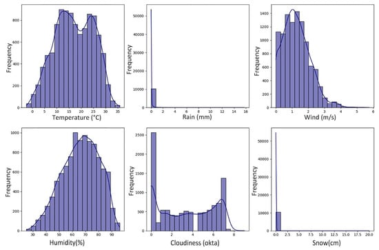
Figure 3.
Weather histogram charts.
Descriptive statistical graphs of the weather factors used in the study are shown in Table 1. The data comprise 10,440 hourly observations, including meteorological variables such as temperature, precipitation, wind speed, humidity, cloudiness, and snow depth.

Table 1.
Weather statistics.
Meteorological parameters, public holidays, and school days were merged to form input variables comprising 10,440 rows. As for school days, the data span the school calendar for primary, middle, and high schools under the 12-year compulsory education system. Due to the large number of universities in Istanbul and the variety of their academic calendars, university school days were excluded.
Figure 4 and Figure 5 provide contour maps visualizing the standard hourly ridership figures for bus lines and railway networks. Areas shaded in red reflect time periods with the highest passenger volumes. In both systems, passenger load clearly increases during morning hours (07:00–09:00) and evening hours (16:00–18:00). The difference in passenger density is more definite on working days, while both systems encounter a decrease in passenger numbers on weekends.
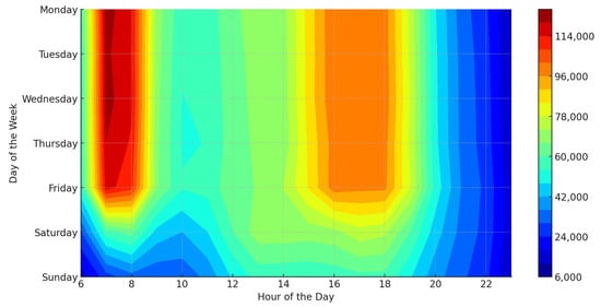
Figure 4.
Hourly average bus public transport ridership heatmap.
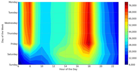
Figure 5.
Hourly average rail transit ridership heatmap.
Table 2 outlines the input variables and their encoded parameters. Temporal variables, public holidays, school days, and meteorological variables are combined. Temporal parameters include month (xM), day of the month (xD), day of the week (xWeek), and hour (xH). These temporal features are considered essential in time series forecasting models, as they help capture recurring patterns in the data. Their inclusion contributes to improved forecasting performance [,]. To account for irregular travel behavior during special days, national holidays (xNH) were also included as input variables []. Likewise, school days (xS) were incorporated, as it has been shown that public transportation usage increases significantly when schools are in session []. Meteorological variables include temperature (xTemperature), precipitation (xRain), snow depth (xSnow), humidity (xHumidity), wind speed (xWind), and cloudiness (xCloudiness). To ensure consistency in data representation, binary variables such as school days and national holidays were represented in binary form, whereas categorical temporal variables such as month, day, and weekday were indexed from 1. The hour variable ranged from 0 to 23 to align with the 24 h clock format commonly used in time series forecasting.
Table 2.
Description of input variables used in the models.
3.2. Feature Importance with XBoost
The XGBoost, an improved version of the Gradient Boosting Decision Tree (GBDT) algorithm, has attracted attention due to its ability to operate in parallel and its efficient use of the boosted tree structure. The XGBoost algorithm is designed to enhance the objective function for regression problems by constructing boosted trees []. In the XGBoost model shown in Equation (1), F signifies the set of decision trees, while n represents the number of data points in the dataset.
Equation (2) presents the objective function. In this function, L, explained in Equation (3), is a differentiable convex loss function that measures the difference between the estimated value and the actual value . The term Ω denotes the regularization term, which serves to avoid overfitting by applying smoothing regularization [].
The XGBoost assesses the importance of a feature using three metrics. The gain metric quantifies how much a feature reduces the error in the model’s splitting decisions within a tree. The frequency metric mirrors how often a feature is used in the model’s split decisions. The cover metric represents the average number of observations influenced by a feature at each split point in the decision tree.
In this study, feature importance was assessed using the gain metric of the XGBoost algorithm. The XGBoost is a model based on gradient-boosted decision trees. The significance of a feature can also be interpreted in terms of how much the model’s predictive performance changes when that feature is randomly perturbed [].
To understand the value of situational and meteorological features in passenger count prediction, the XGBoost model was employed. The model’s hyperparameters were adjusted to minimize the RMSE error metric, as presented in Table 3.
Table 3.
Optimal hyperparameters for XGBoost.
As shown in Figure 6, the hour variable appeared as the most important feature. This was followed by school days, day of the week, public holidays, and month. Among meteorological variables, humidity, temperature, and wind speed had relatively lower importance compared to time-related variables. Precipitation, snow depth, day of the month, and cloud cover were identified as features with the lowest importance. In deep learning-based approaches, improving predictive accuracy and reducing model complexity by eliminating unnecessary parameters is essential. Therefore, based on the feature importance ranking, the variables that contributed most significantly—hour, school days, day of the week, public holidays, month, humidity, temperature, and wind speed—were selected as input features for the modeling process.
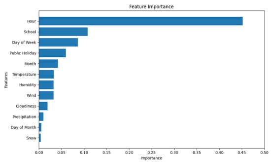
Figure 6.
Importance of the input parameters in the XGBoost model.
The limited influence of precipitation- and snow-related variables may be attributed to the relatively low number of rainy or snowy days during the study period. This constraint may have hindered the model’s ability to learn the relationship between these features and passenger flow, leading to their lower rankings in the feature importance analysis.
3.3. Proposed Model Architecture
Two data types are relied upon for the predictive performance of the proposed models: temporal variables and external meteorological parameters. These two databases were merged to form a combined dataset consisting of 10,440 hourly records. To handle missing values, the K-Nearest Neighbors (KNN) approach was implemented, which estimates missing observations based on the overall patterns within the dataset []. Once the data were prepared, it was separated into training and testing sets in an 80:20 ratio. Because model performance is highly influenced by the accuracy of data standardization, the Min-Max normalization method was applied during the preprocessing phase prior to constructing the models []. Subsequently, all variables were scaled using this method to ensure consistency across the datasets.
In the next phase, the LSTM model was initially used to predict passenger flow for bus and train services, based on selected parameters. Subsequently, to identify the best-performing model, three additional state-of-the-art deep learning models—RNN, GRU, and NARX—were incorporated for comparative analysis. Figure 7 displays a visual representation of the methodological framework and forecasting steps of this study.
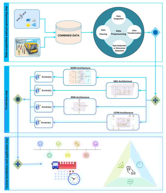
Figure 7.
Flowchart of the forecasting model.
Among deep learning methods, RNN, LSTM, and GRU architectures hold a central position in passenger flow forecasting. The LSTM model was selected due to its proven effectiveness in capturing temporal dependencies in sequential data. Its ability to retain relevant information over extended periods renders it highly effective for modeling the dynamic and nonlinear nature of public transportation demand [,,]. The GRU model, on the other hand, was included in the study as a more computationally efficient alternative to LSTM. GRU has proven effective in short-term forecasting tasks, especially in contexts with frequent intra-day variability, and has yielded accurate passenger flow forecasts []. Although the NARX model has been prevalent in fields such as energy forecasting and load prediction, its application to short-term public transport passenger flow has been scarcely addressed [,]. Considering its ability to integrate external inputs and historical values, the NARX architecture was selected to examine whether its superior performance in other domains could be replicated in the context of public transportation. This model was included to investigate an underexplored method and to compare its effectiveness with more commonly used deep learning models such as LSTM, GRU, and RNN.
The widely used RNN architecture is adopted by this study for time series data, and it performs a thorough analysis using LSTM, GRU, and NARX models, which are adept at capturing long-term dependencies.
To prevent overfitting during training, early stopping and a learning rate adaptation strategy that reduces the learning rate when the validation performance plateaus (ReduceLROnPlateau) were employed. These techniques were adopted to enhance both the generalization capability of the models and the efficiency of the training process.
3.4. Error Metrics
To assess the performance of the DL models, several statistical error metrics were used, such as the following:
RMSE, described in Equation (4), calculates the square root of the mean of squared differences between predicted and actual values. Higher prediction accuracy is shown by lower RMSE values. MAPE, presented in Equation (5), measures the average percentage difference between predicted and actual values. Standard Deviation of Absolute Errors (StdAE), shown in Equation (6), evaluates the variability of prediction errors by calculating the Standard Deviation of Absolute Errors (AE). The Relative Absolute Error (RAE), defined in Equation (7), compares the model’s performance to the mean prediction error, providing a comparative performance assessment. The Standard Deviation of Absolute Percentage Errors (StdAPE), given in Equation (8), expresses the variation values in APE (Absolute Percentage Error), providing insights into the dependability of the model’s predictions [,].
3.5. RNN
RNNs are capable of modeling short-term temporal dependencies in passenger flow prediction. RNNs generate predictions by taking into account prior input values. In Figure 8, mirrors the model input at time as is the hidden state at time with representing the predicted value for that specific time [].
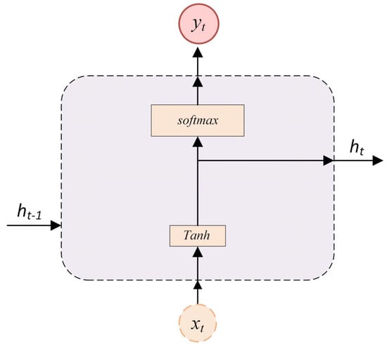
Figure 8.
Basic architecture of the RNN model.
RNNs typically consist of multiple layers of neurons that process and propagate outputs from one layer to the next, thereby capturing dependencies in sequential data over time.
3.6. LSTM
The LSTM model offers an effective solution to the vanishing gradient problem often encountered in RNNs []. As a specialized form of RNN, LSTM networks are capable of retaining relevant information over extended sequences, making them well-suited for modeling time series data. LSTMs utilize memory cells to store information and selectively update or forget it as needed. Figure 9 illustrates the architecture of a basic LSTM model [].
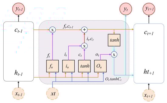
Figure 9.
Basic architecture of the LSTM model.
LSTM units are structured with three distinct gates: the input gate , the forget gate , and the output gate , each of which receives a value between 0 and 1. The input gate governs the integration of selected features into the memory. The forget gate discards information deemed unnecessary, whereas the output gate decides the value to be produced by the unit. These gates operate based on both the previous hidden state − 1) and the current input , collectively influencing the unit’s output. These formulas are defined in Equations (9)–(11) [].
The weight matrices , , , , , , , and correspond to the weight parameters related to the current input and the previous hidden state for their respective gates. Bias parameters for the forget, input, output, and cell gates are expressed as , , respectively. The notation σ designates the sigmoid activation function. The input gate , forget gate , the previous cell state (), and the candidate cell state all contribute to calculating the updated cell state . After establishing the updated cell state, the output state can be calculated as detailed in Equations (12)–(14).
3.7. GRU
GRU offers a simpler alternative to the LSTM architecture while maintaining similar performance. As illustrated in Figure 10, a standard GRU cell features two main gates: the reset gate (), responsible for regulating the influence of the previous state, and the update gate (), which decides the extent to which past information is preserved in the current state. Additionally, based on the reset gate, a candidate hidden state () is computed, as expressed in Equation (17). The final output of the GRU cell, , is given in Equation (18). Unlike LSTM, the GRU combines the functionalities of the input and forget gates into a single update gate () [,].
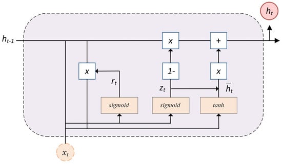
Figure 10.
GRU cell architecture.
3.8. NARX
The NARX model is a recurrent neural network that extends a feedforward architecture by integrating feedback through dynamic recurrent connections. The NARX model is particularly effective in forecasting future values of a time series based on its past inputs and outputs. It achieves this by incorporating a delay mechanism for both input and output variables. By means of this feature, it yields significant results in the estimation of nonlinear relationships. In this model, x(n) and y(n) represent the input and output values at time n, respectively. The parameter dE denotes the maximum delay for inputs, while dy denotes the maximum delay for outputs. Figure 11 illustrates the architecture of the NARX model [,].
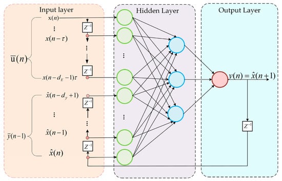
Figure 11.
NARX architecture diagram.
The hidden layer of the NARX model employs a sigmoid activation function, whereas the output layer uses a linear activation function []. The sigmoid function used in the hidden layer is defined in Equation (21).
For model training, a gradient-based backpropagation algorithm is utilized, enabling parameter updates and error minimization. The capacity of the model to learn the nonlinear structure of the time series is enhanced through the use of delay structures in both the input and output layers.
In this model, datasets are constructed from the time-delayed values of x(n) and output data y(n) []. Subsequently, the data are divided into training and testing sets, and the model’s performance is evaluated using error metrics. DL models often require tuning numerous hyperparameters to achieve high accuracy, with performance varying considerably across different configurations []. For the models presented in Table 4 and Table 5, various hyperparameter combinations are explored, and the hyperparameters that yield the highest prediction performance are identified through comprehensive analysis.
Table 4.
Optimum hyperparameters for the models.
Table 5.
Optimum hyperparameters for the NARX model.
4. Experimental Results
According to Table 6, in the LSTM prediction model developed using combinations of weather parameters for the bus lines operating along the Kadıköy–Pendik route, the inclusion of temperature and wind speed values from one hour prior led to a 3.7% reduction in RMSE compared to the model without weather variables. Higher MAPE values were observed during weekends and off-peak hours, a pattern also found in rail systems. In contrast, weekday and peak-hour predictions demonstrated more stable and balanced estimates. In Table 7, Table 8, Table 9, Table 10 and Table 11, the symbol 🗸 indicates the presence of a variable, X denotes its absence, and bold values highlight the best performance results.
Table 6.
Public bus transportation on the Kadıköy–Pendik route.
Table 7 presents findings for two rail systems (M4 Metro and B1 Gebze–Üsküdar Line) along the Kadıköy–Pendik corridor. In scenarios where temperature and wind speed from one hour earlier were included in the LSTM model, the RMSE reached its lowest level, achieving a 2.5% improvement over models using only temporal variables. However, an increase in MAPE was noted during weekends and off-peak hours, suggesting higher percentage error rates during those periods. Additionally, the RMSE values obtained for bus passenger flow predictions were found to be lower than those for rail lines, indicating that bus traffic might be more responsive to short-term fluctuations and thus more effectively modeled.
Table 7.
Public rail transportation on the Kadıköy–Pendik route.
Table 7.
Public rail transportation on the Kadıköy–Pendik route.
| Input Variables | LSTM | |||||||||
|---|---|---|---|---|---|---|---|---|---|---|
| Model | Temporal | xTemp | xHumidity | xWind | MAPE | RMSE | TIC | STD_AE | RAE | STD_APE |
| 1 | 🗸 | X | X | X | 0.05384 | 2165 | 0.0292 | 1598 | 0.112 | 7.448 |
| 2 | 🗸 | 🗸 | X | X | 0.0609 | 2318 | 0.0314 | 1661 | 0.1241 | 8.244 |
| 3 | 🗸 | 🗸 | X | 🗸 | 0.0534 | 2133 | 0.0291 | 1577 | 0.111 | 7.408 |
| 4 | 🗸 | X | X | 🗸 | 0.0641 | 2494 | 0.033 | 1786 | 0.133 | 8.096 |
| 5 | 🗸 | 🗸 | 🗸 | X | 0.0594 | 2365 | 0.032 | 1720 | 0.1245 | 8.511 |
| 6 | 🗸 | X | 🗸 | 🗸 | 0.056 | 2219 | 0.03 | 1614 | 0.1168 | 9.186 |
| 7 | 🗸 | X | 🗸 | X | 0.0554 | 2342 | 0.0319 | 1712 | 0.122 | 7.283 |
| 8 | 🗸 | 🗸 | 🗸 | 🗸 | 0.0559 | 2232 | 0.0303 | 1625 | 0.1175 | 7.200 |
| Previous Hour Input Variables | LSTM | |||||||||
| Model | Temporal | xTemp | xHumidity | xWind | MAPE | RMSE | TIC | STD_AE | RAE | STD_APE |
| 1 | 🗸 | X | X | X | 0.05384 | 2165 | 0.0292 | 1598 | 0.112 | 7.448 |
| 2 | 🗸 | 🗸 | X | X | 0.0584 | 2271 | 0.0309 | 1603 | 0.1234 | 6.687 |
| 3 | 🗸 | 🗸 | X | 🗸 | 0.051 | 2112 | 0.0279 | 1508 | 0.1085 | 6.762 |
| 4 | 🗸 | X | X | 🗸 | 0.059 | 2260 | 0.0306 | 1575 | 0.1243 | 8.940 |
| 5 | 🗸 | 🗸 | 🗸 | X | 0.0608 | 2286 | 0.031 | 1618 | 0.124 | 8.159 |
| 6 | 🗸 | X | 🗸 | 🗸 | 0.06346 | 2392 | 0.0325 | 1683 | 0.1305 | 8.836 |
| 7 | 🗸 | X | 🗸 | X | 0.06883 | 2546 | 0.0347 | 1768 | 0.1406 | 9.955 |
| 8 | 🗸 | 🗸 | 🗸 | 🗸 | 0.0562 | 2299 | 0.0312 | 1694 | 0.119 | 9.791 |
| MAPE | RMSE | TIC | STD_AE | RAE | STD_APE | |||||
| Weekend | 0.071 | 2101 | 0.0347 | 1540 | 0.1278 | 10.347 | ||||
| Weekday | 0.0487 | 2177 | 0.0277 | 1584 | 0.1104 | 5.710 | ||||
| Peak hours | 0.0443 | 2620 | 0.027 | 1835 | 0.1517 | 4.733 | ||||
| Off peak | 0.0621 | 1798 | 0.0335 | 1317 | 0.1452 | 8.653 | ||||
In Table 8, findings for all bus routes serving the Asian side of Istanbul showed that incorporating one-hour lagged temperature and wind speed variables into the LSTM model yielded the lowest RMSE values, similar to the results observed on the Kadıköy–Pendik route. Nevertheless, the percentage improvement in RMSE was more limited compared to the Kadıköy–Pendik corridor.
Table 8.
Public bus transportation on the Asian side of Istanbul.
Table 8.
Public bus transportation on the Asian side of Istanbul.
| Input Variables | LSTM | |||||||||
|---|---|---|---|---|---|---|---|---|---|---|
| Model | Temporal | xTemp | xHumidity | xWind | MAPE | RMSE | TIC | STD_AE | RAE | STD_APE |
| 1 | 🗸 | X | X | X | 0.0389 | 3738 | 0.0228 | 2701 | 0.091 | 4.183 |
| 2 | 🗸 | 🗸 | X | X | 0.04 | 3760 | 0.023 | 2665 | 0.0916 | 4.518 |
| 3 | 🗸 | 🗸 | X | 🗸 | 0.0384 | 3687 | 0.022 | 2698 | 0.088 | 4.508 |
| 4 | 🗸 | X | X | 🗸 | 0.041 | 3830 | 0.0234 | 2802 | 0.0922 | 4.696 |
| 5 | 🗸 | 🗸 | 🗸 | X | 0.051 | 4095 | 0.025 | 2776 | 0.106 | 5.984 |
| 6 | 🗸 | X | 🗸 | 🗸 | 0.0499 | 4172 | 0.0256 | 2875 | 0.106 | 6.232 |
| 7 | 🗸 | X | 🗸 | X | 0.049 | 4193 | 0.0258 | 2901 | 0.1067 | 5.302 |
| 8 | 🗸 | 🗸 | 🗸 | 🗸 | 0.0461 | 4106 | 0.0254 | 2888 | 0.1036 | 4.545 |
| Previous Hour Input Variables | LSTM | |||||||||
| Model | Temporal | xTemp | xHumidity | xWind | MAPE | RMSE | TIC | STD_AE | RAE | STD_APE |
| 1 | 🗸 | X | X | X | 0.0389 | 3738 | 0.0228 | 2701 | 0.091 | 4.183 |
| 2 | 🗸 | 🗸 | X | X | 0.0406 | 3748 | 0.0231 | 2711 | 0.0927 | 5.052 |
| 3 | 🗸 | 🗸 | X | 🗸 | 0.0378 | 3655 | 0.0218 | 2690 | 0.087 | 4.498 |
| 4 | 🗸 | X | X | 🗸 | 0.0415 | 3800 | 0.0233 | 2764 | 0.092 | 4.668 |
| 5 | 🗸 | 🗸 | 🗸 | X | 0.0496 | 4014 | 0.024 | 2732 | 0.103 | 7.315 |
| 6 | 🗸 | X | 🗸 | 🗸 | 0.0485 | 4137 | 0.0253 | 2905 | 0.104 | 5.134 |
| 7 | 🗸 | X | 🗸 | X | 0.0452 | 4084 | 0.0251 | 2910 | 0.1 | 4.545 |
| 8 | 🗸 | 🗸 | 🗸 | 🗸 | 0.0456 | 3962 | 0.0242 | 2781 | 0.099 | 4.907 |
| MAPE | RMSE | TIC | STD_AE | RAE | STD_APE | |||||
| Weekend | 0.0452 | 2659 | 0.0234 | 1813 | 0.1019 | 5.848 | ||||
| Weekday | 0.0349 | 3856 | 0.0215 | 2846 | 0.0901 | 4.033 | ||||
| Peak hours | 0.0318 | 3958 | 0.0189 | 2621 | 0.1045 | 3.435 | ||||
| Off peak | 0.0417 | 3265 | 0.026 | 2535 | 0.0934 | 5.253 | ||||
As shown in Table 9, for the three rail lines on Istanbul’s Asian side (M4 and M5 metro lines, and the B1 Gebze–Üsküdar commuter line), various combinations of weather parameters were evaluated in the LSTM model. Although a decrease in RMSE was observed when using one-hour prior temperature and wind speed, the percentage improvement remained below 1%. This suggests that the contribution of these parameters to model performance is relatively marginal in this context.
Table 9.
Public rail transportation on the Asian side of Istanbul.
Table 9.
Public rail transportation on the Asian side of Istanbul.
| Input Variables | LSTM | |||||||||
|---|---|---|---|---|---|---|---|---|---|---|
| Model | Temporal | xTemp | xHumidity | xWind | MAPE | RMSE | TIC | STD_AE | RAE | STD_APE |
| 1 | 🗸 | X | X | X | 0.0569 | 3268 | 0.0303 | 2421 | 0.1105 | 8.845 |
| 2 | 🗸 | 🗸 | X | X | 0.0551 | 3452 | 0.032 | 2592 | 0.114 | 7.637 |
| 3 | 🗸 | 🗸 | X | 🗸 | 0.0549 | 3240 | 0.0301 | 2417 | 0.10926 | 8.084 |
| 4 | 🗸 | X | X | 🗸 | 0.0565 | 3324 | 0.0308 | 2455 | 0.112 | 8.266 |
| 5 | 🗸 | 🗸 | 🗸 | X | 0.0569 | 3401 | 0.0317 | 2468 | 0.1178 | 7.640 |
| 6 | 🗸 | X | 🗸 | 🗸 | 0.0548 | 3405 | 0.031 | 2527 | 0.115 | 9.077 |
| 7 | 🗸 | X | 🗸 | X | 0.0597 | 3690 | 0.0345 | 2710 | 0.1262 | 7.138 |
| 8 | 🗸 | 🗸 | 🗸 | 🗸 | 0.0639 | 3580 | 0.0335 | 2521 | 0.128 | 7.237 |
| Previous Hour Input Variables | LSTM | |||||||||
| Model | Temporal | xTemp | xHumidity | xWind | MAPE | RMSE | TIC | STD_AE | RAE | STD_APE |
| 1 | 🗸 | X | X | X | 0.0569 | 3268 | 0.0303 | 2421 | 0.1105 | 8.845 |
| 2 | 🗸 | 🗸 | X | X | 0.0569 | 3338 | 0.031 | 2412 | 0.116 | 7.409 |
| 3 | 🗸 | 🗸 | X | 🗸 | 0.0545 | 3258 | 0.0301 | 2418 | 0.103 | 7.982 |
| 4 | 🗸 | X | X | 🗸 | 0.0573 | 3383 | 0.0313 | 2472 | 0.1163 | 7.649 |
| 5 | 🗸 | 🗸 | 🗸 | X | 0.0578 | 3427 | 0.032 | 2513 | 0.1173 | 8.752 |
| 6 | 🗸 | X | 🗸 | 🗸 | 0.0575 | 3550 | 0.0333 | 2603 | 0.121 | 9.904 |
| 7 | 🗸 | X | 🗸 | X | 0.0624 | 3702 | 0.0347 | 2627 | 0.131 | 7.782 |
| 8 | 🗸 | 🗸 | 🗸 | 🗸 | 0.0623 | 3654 | 0.0341 | 2658 | 0.1263 | 8.641 |
| MAPE | RMSE | TIC | STD_AE | RAE | STD_APE | |||||
| Weekend | 0.0652 | 3136 | 0.0362 | 2324 | 0.1275 | 10.544 | ||||
| Weekday | 0.0486 | 3485 | 0.0303 | 2580 | 0.112 | 4.913 | ||||
| Peak hours | 0.0479 | 4390 | 0.0306 | 3104 | 0.1669 | 4.612 | ||||
| Off peak | 0.057 | 2550 | 0.0334 | 1860 | 0.144 | 8.237 | ||||
4.1. Comparison of Model Performance
To thoroughly evaluate the performance of the LSTM forecasting model developed in this study, comparisons were conducted with other commonly used deep learning and artificial intelligence-based models, namely RNN, GRU, and NARX. The impact of weather variables—particularly temperature and wind—on passenger flow prediction was previously examined in detail within the LSTM framework. All comparison models are widely accepted AI algorithms with proven success in various time series forecasting tasks. To ensure a fair comparison, all models were trained using identical input variables and data samples under equivalent conditions. Due to the greater RMSE improvements observed for the Kadıköy–Pendik route compared to the broader Asian side, temperature and wind data from one hour prior were included in all models as supplementary temporal features. LSTM, GRU RNN, and NARX models were subsequently analyzed comparatively using this enhanced input structure.
The results presented in Table 10 and Table 11 reveal that the NARX model consistently achieved the lowest MAPE and RMSE values across both datasets, thereby delivering the most accurate forecasting performance. These findings highlight the NARX model as a particularly strong candidate for short-term passenger flow forecasting.
Table 10.
Model predictions for bus public transit: Kadıköy–Pendik route.
Table 10.
Model predictions for bus public transit: Kadıköy–Pendik route.
| Model | MAPE | RMSE | TIC | STD_AE | RAE | STD_APE |
|---|---|---|---|---|---|---|
| LSTM | 0.0474 | 542 | 0.024 | 364 | 0.1032 | 5.517 |
| GRU | 0.0488 | 544 | 0.024 | 359 | 0.105 | 5.447 |
| RNN | 0.0568 | 634 | 0.0282 | 431 | 0.119 | 7.244 |
| NARX | 0.042 | 449 | 0.022 | 311 | 0.0947 | 5.267 |
Table 11.
Model predictions for rail public transit: Kadıköy–Pendik route.
Table 11.
Model predictions for rail public transit: Kadıköy–Pendik route.
| Model | MAPE | RMSE | TIC | STD_AE | RAE | STD_APE |
|---|---|---|---|---|---|---|
| LSTM | 0.051 | 2112 | 0.0279 | 1508 | 0.108 | 6.762 |
| GRU | 0.0615 | 2366 | 0.0322 | 1698 | 0.126 | 8.707 |
| RNN | 0.0845 | 4074 | 0.0565 | 3045 | 0.207 | 10.690 |
| NARX | 0.0459 | 1753 | 0.0257 | 1281 | 0.099 | 6.491 |
4.2. Significance Test
To compare the forecasting performance of the different models, non-parametric statistical tests were employed. Specifically, the Friedman test—a post hoc method—was used to identify statistically significant differences among the algorithms. The corresponding Friedman statistics are provided in Table 12. In cases where the p-value was less than 0.05, the null hypothesis—stating that the models’ average performances were equal—was rejected. This result indicates that at least one of the models performed significantly better than the others, confirming the presence of statistically meaningful differences among them.
Table 12.
Post hoc results of the Friedman test.
5. Discussion
The analyses revealed that the humidity parameter did not make a significant contribution to passenger demand prediction performance in any of the models. Similarly, temperature had a limited effect, particularly in bus passenger forecasting. In contrast, when wind speed was incorporated into the model alongside temperature with a one-hour lag, it led to a 2.2% reduction in RMSE at the regional level for bus forecasts on the Asian side and a 2.4% reduction for rail systems at the route level. While these results indicate slight improvements, they suggest that the influence of weather variables is generally limited in such contexts. However, on the Kadıköy–Pendik route, the same combination resulted in a 3.69% decrease in RMSE, representing a more meaningful enhancement in predictive accuracy. This finding highlights that, although the overall contribution of weather-related variables may be modest, their impact can become more pronounced under specific spatial and operational conditions.
It should also be noted that the dataset used in this study covers only a 1.5-year time span, which limits the ability to identify statistically significant seasonal cycles. As such, the full potential of weather-related variables in improving model accuracy may not have been fully realized.
One possible explanation for the relatively smaller impact of weather variables on railway passenger flow compared to bus systems could be the difference in infrastructure. Unlike open-air bus stops, train stations generally provide sheltered environments that protect passengers from adverse weather conditions. Moreover, while accessing bus stops often requires walking through open or unprotected areas, train stations are typically integrated into larger transportation hubs or enclosed structures, offering greater protection and comfort regardless of the weather. In particular, passengers using underground metro stations are less likely to be affected by extreme weather events due to the enclosed nature of the infrastructure [,].
The limited impact of precipitation- and snow-related variables observed in this study may be attributed to the relatively low number of rainy and snowy days in the dataset. This data scarcity may have restricted the model’s ability to learn the relationship between such weather conditions and passenger flow, resulting in their low ranking in the feature importance analysis. However, in regions with higher levels of precipitation, the impact of these variables on model performance may be more substantial. To address these gaps, future studies conducted in different climatic settings and based on longer data periods could better capture the influence of adverse weather conditions on public transport demand.
Across all models, the StdAPE values were higher than the MAPE values. This discrepancy can be linked to more noticeable deviations in scenarios with low passenger volumes. Lowering StdAPE would contribute to more consistent forecasts. The analysis also stressed that error rates were proportionally higher during off-peak periods, suggesting that special attention should be given to enhancing predictions during these hours.
Among the four models built for predicting bus and rail passenger volumes, the NARX outperformed the others, yielding the lowest MAPE and RMSE values. These findings indicate the superior predictive accuracy of the NARX model in short-term forecasting tasks.
Uncertainty in weather forecasts can also directly affect the accuracy of passenger flow predictions. While short-term forecasts (1–7 days: high accuracy; 8–10 days: moderate accuracy; 11–14 days: low accuracy) are generally more reliable [], they can introduce significant uncertainty in long-term scenarios. Consequently, the models developed in this study are best suited for short-term forecasting applications. Certain limitations should be acknowledged. Firstly, the smart card data used were aggregated at hourly intervals, whereas public transport services typically operate at 5–30 min intervals, which may limit forecasting precision. Analyses based on minute-level data could enable more refined and detailed predictions.
Secondly, although the deep learning models used in this study are effective in capturing short-term fluctuations, they exhibit limitations in modeling long-term trends and seasonal patterns. This limitation primarily stems from the relatively short time span of the dataset (1.5 years), which makes it difficult to identify statistically significant seasonal cycles. Classical ARIMA approaches tend to show limited performance when applied to high-frequency (e.g., hourly) and multivariate datasets, particularly in terms of accuracy, computational efficiency, and sensitivity to data quality []. Therefore, traditional models were not included in this study. In future studies, it would be beneficial to extend the dataset over multiple years and increase the data coverage, in addition to employing hybrid models that combine statistical seasonal forecasting methods with deep learning architectures, in order to better capture seasonality.
6. Conclusions
This study has revealed that specific weather parameters can significantly impact passenger demand forecasts in public transportation systems. Employing 1.5 years of smart card and meteorological data from 2021 to 2022, passenger numbers for both bus and rail systems were estimated through deep learning models for Istanbul’s Asian side and the Kadıköy–Pendik corridor. The key findings are summarized below:
- Deep learning-based models have produced successful results, particularly in predicting both bus and rail passenger flows.
- The highest forecasting accuracy among weather variables was achieved when both temperature and wind speed from one hour earlier were included in the model. However, when considered alone, these parameters did not demonstrate significant effects when considered independently.
- The models produced more stable predictions during weekdays and peak hours, while forecasting performance dropped during weekends and off-peak periods due to increased fluctuations in passenger volume.
- Route-based rail models that include temperature and wind speed provided a modest improvement in RMSE of 2.4%.
- In region-based bus forecasts, a modest 2.2% reduction in RMSE was observed on the Asian side, while a larger improvement of 3.69% was achieved on the Kadıköy–Pendik route.
The main aim of the study was to develop short-term forecasts for bus and rail passenger volumes along the same region and route, including weather conditions. The incorporation of weather variables enhanced the prediction performance for buses; however, their effect on the rail system was minimal. In future studies, the timing of mass events such as football matches and concerts could be incorporated as external variables to mitigate sudden fluctuations during weekends and low-demand periods. Furthermore, using smart card data with minute-level granularity could improve model sensitivity, while extending the time span of the dataset would enhance the model’s ability to capture seasonal effects. The use of model explanation techniques such as SHAP (SHapley Additive exPlanations) alongside XGBoost-based feature selection could provide a more comprehensive understanding of feature contributions. As a result, this integration may enhance the interpretability and transparency of forecasting models, thereby enabling a more accurate assessment of both model reliability and performance []. The findings support transportation planners in making more informed, data-driven decisions regarding scheduling, capacity management, and service optimization.
Author Contributions
Conceptualization: C.Y. and A.P.A.; methodology: C.Y. and A.P.A.; software: C.Y.; validation: C.Y. and A.P.A.; formal analysis: C.Y.; investigation: A.P.A. and C.Y.; data curation: C.Y.; writing—original draft preparation: C.Y.; writing—review and editing: C.Y. and A.P.A.; visualization: C.Y.; supervision: A.P.A. All authors have read and agreed to the published version of the manuscript.
Funding
This research received no external funding.
Institutional Review Board Statement
Not applicable.
Informed Consent Statement
Not applicable.
Data Availability Statement
The original contributions presented in this study are included in the article. Further inquiries can be directed to the corresponding author.
Conflicts of Interest
The authors declare no conflicts of interest.
References
- Javid, M.A.; Ali, N.; Hussain Shah, S.A.; Abdullah, M. Travelers’ Attitudes Toward Mobile Application–Based Public Transport Services in Lahore. Sage Open 2021, 11, 2158244020988709. [Google Scholar] [CrossRef]
- Anderson, M.L. Subways, Strikes, and Slowdowns: The Impacts of Public Transit on Traffic Congestion. Am. Econ. Rev. 2014, 104, 2763–2796. [Google Scholar] [CrossRef]
- Gentile, G.; Florian, M.; Hamdouch, Y.; Cats, O.; Nuzzolo, A. The Theory of Transit Assignment: Basic Modelling Frameworks. In Modelling Public Transport Passenger Flows in the Era of Intelligent Transport Systems: COST Action TU1004 (TransITS); Gentile, G., Noekel, K., Eds.; Springer International Publishing: Cham, Switzerland, 2016; pp. 287–386. ISBN 978-3-319-25082-3. [Google Scholar]
- Hwang, M.; Kemp, J.; Lerner-Lam, E.; Neuerburg, N.; Okunieff, P.E.; Palisades Group International; Omni Group. Advanced Public Transportation Systems: The State of the Art Update 2006; U.S. Department of Transportation: Washington, DC, USA, 2006. [Google Scholar]
- Baghbani, A.; Bouguila, N.; Patterson, Z. Short-Term Passenger Flow Prediction Using a Bus Network Graph Convolutional Long Short-Term Memory Neural Network Model. Transp. Res. Rec. 2023, 2677, 1331–1340. [Google Scholar] [CrossRef]
- Ma, Z.; Xing, J.; Mesbah, M.; Ferreira, L. Predicting Short-Term Bus Passenger Demand Using a Pattern Hybrid Approach. Transp. Res. Part C Emerg. Technol. 2014, 39, 148–163. [Google Scholar] [CrossRef]
- Castillo, E.; Menéndez, J.M.; Sánchez-Cambronero, S. Predicting Traffic Flow Using Bayesian Networks. Transp. Res. Part B Methodol. 2008, 42, 482–509. [Google Scholar] [CrossRef]
- Smith, B.L.; Williams, B.M.; Keith Oswald, R. Comparison of Parametric and Nonparametric Models for Traffic Flow Forecasting. Transp. Res. Part C Emerg. Technol. 2002, 10, 303–321. [Google Scholar] [CrossRef]
- Zhang, Y.; Liu, Y. Traffic Forecasting Using Least Squares Support Vector Machines. Transportmetrica 2009, 5, 193–213. [Google Scholar] [CrossRef]
- Zhu, D.; Du, H.; Sun, Y.; Cao, N. Research on Path Planning Model Based on Short-Term Traffic Flow Prediction in Intelligent Transportation System. Sensors 2018, 18, 4275. [Google Scholar] [CrossRef]
- Sun, S.; Zhang, C.; Yu, G. A Bayesian Network Approach to Traffic Flow Forecasting. IEEE Trans. Intell. Transp. Syst. 2006, 7, 124–132. [Google Scholar] [CrossRef]
- Zhang, F.; Zhu, X.; Hu, T.; Guo, W.; Chen, C.; Liu, L. Urban Link Travel Time Prediction Based on a Gradient Boosting Method Considering Spatiotemporal Correlations. ISPRS Int. J. Geo-Inf. 2016, 5, 201. [Google Scholar] [CrossRef]
- Ahmed, M.S.; Cook, A.R. Analysis of Freeway Traffic Time-Series Data by Using Box-Jenkins Techniques. In Urban Systems Operations; Transportation Research Board: Washington, DC, USA, 1979. [Google Scholar]
- Williams, B.M.; Hoel, L.A. Modeling and Forecasting Vehicular Traffic Flow as a Seasonal ARIMA Process: Theoretical Basis and Empirical Results. J. Transp. Eng. 2003, 129, 664–672. Available online: https://ascelibrary.org/doi/abs/10.1061/(ASCE)0733-947X(2003)129:6(664) (accessed on 15 November 2024). [CrossRef]
- Ye, Y.; Chen, L.; Xue, F. Passenger Flow Prediction in Bus Transportation System Using ARIMA Models with Big Data. In Proceedings of the 2019 International Conference on Cyber-Enabled Distributed Computing and Knowledge Discovery (CyberC), Guilin, China, 17–19 October 2019; pp. 436–443. [Google Scholar]
- Gu, Y.; Lu, W.; Xu, X.; Qin, L.; Shao, Z.; Zhang, H. An Improved Bayesian Combination Model for Short-Term Traffic Prediction With Deep Learning. IEEE Trans. Intell. Transp. Syst. 2020, 21, 1332–1342. [Google Scholar] [CrossRef]
- Liang, S.; Ma, M.; He, S.; Zhang, H. Short-Term Passenger Flow Prediction in Urban Public Transport: Kalman Filtering Combined K-Nearest Neighbor Approach. IEEE Access 2019, 7, 120937–120949. [Google Scholar] [CrossRef]
- Jiao, P.; Li, R.; Sun, T.; Hou, Z.; Ibrahim, A. Three Revised Kalman Filtering Models for Short-Term Rail Transit Passenger Flow Prediction. Math. Probl. Eng. 2016, 2016, 9717582. [Google Scholar] [CrossRef]
- Chuwang, D.D.; Chen, W. Forecasting Daily and Weekly Passenger Demand for Urban Rail Transit Stations Based on a Time Series Model Approach. Forecasting 2022, 4, 904–924. [Google Scholar] [CrossRef]
- Photun, A.; Thaminkaew, T. Forecasting Air Passengers in Phuket, Thailand: An Application of Machine Learning Algorithms. In Proceedings of the 2023 4th International Conference on Big Data Analytics and Practices (IBDAP), Bangkok, Thailand, 25–27 August 2023; pp. 1–6. [Google Scholar]
- Liu, S.; Yao, E. Holiday Passenger Flow Forecasting Based on the Modified Least-Square Support Vector Machine for the Metro System. J. Transp. Eng. Part A Syst. 2017, 143, 04016005. [Google Scholar] [CrossRef]
- Vlahogianni, E.I.; Karlaftis, M.G.; Golias, J.C. Optimized and Meta-Optimized Neural Networks for Short-Term Traffic Flow Prediction: A genetic approach. Transp. Res. Part C Emerg. Technol. 2005, 13, 211–234. [Google Scholar] [CrossRef]
- Çelebi, S.B.; Emiroğlu, B.G. A Novel Deep Dense Block-Based Model for Detecting Alzheimer’s Disease. Appl. Sci. 2023, 13, 8686. [Google Scholar] [CrossRef]
- Bharti; Redhu, P.; Kumar, K. Short-Term Traffic Flow Prediction Based On Optimized Deep Learning Neural Network: PSO-Bi-LSTM. Phys. A Stat. Mech. Its Appl. 2023, 625, 129001. [Google Scholar] [CrossRef]
- Janiesch, C.; Zschech, P.; Heinrich, K. Machine learNing and Deep Learning. Electron. Mark. 2021, 31, 685–695. [Google Scholar] [CrossRef]
- Çelebi, S.B.; Emiroğlu, B.G. Leveraging Deep Learning for Enhanced Detection of Alzheimer’s Disease Through Morphometric Analysis of Brain Images, IIETA. Trait. Du Signal 2023, 40, 1355–1365. Available online: https://www.iieta.org/journals/ts/paper/10.18280/ts.400405 (accessed on 28 April 2025). [CrossRef]
- Han, J.; Kim, J.; Kim, S.; Wang, S. Effectiveness of Image Augmentation Techniques on Detection of Building Characteristics from Street View Images Using Deep Learning. J. Constr. Eng. Manag. 2024, 150, 04024129. [Google Scholar] [CrossRef]
- Haykin, S.; Kosko, B. GradientBased Learning Applied to Document Recognition. In Intelligent Signal Processing; Wiley-IEEE Press: Piscataway, New Jersey, USA, 2001; pp. 306–351. ISBN 978-0-470-54497-6. [Google Scholar]
- Birecikli, B.; Karaman, Ö.A.; Çelebi, S.B.; Turgut, A. Failure Load Prediction of Adhesively Bonded GFRP Composite Joints Using Artificial Neural Networks. J. Mech. Sci. Technol. 2020, 34, 4631–4640. [Google Scholar] [CrossRef]
- Karaman, Ö.A. Prediction of Wind Power with Machine Learning Models. Appl. Sci. 2023, 13, 11455. [Google Scholar] [CrossRef]
- Shobayo, O.; Adeyemi-Longe, S.; Popoola, O.; Okoyeigbo, O. A Comparative Analysis of Machine Learning and Deep Learning Techniques for Accurate Market Price Forecasting. Analytics 2025, 4, 5. [Google Scholar] [CrossRef]
- Xiong, Z.; Zheng, J.; Song, D.; Zhong, S.; Huang, Q. Passenger Flow Prediction of Urban Rail Transit Based on Deep Learning Methods. Smart Cities 2019, 2, 371–387. [Google Scholar] [CrossRef]
- Halyal, S.; Mulangi, R.H.; Harsha, M.M. Forecasting Public Transit Passenger Demand: With Neural Networks Using APC Data. Case Stud. Transp. Policy 2022, 10, 965–975. [Google Scholar] [CrossRef]
- Cheng, C.-H.; Tsai, M.-C.; Cheng, Y.-C. An Intelligent Time-Series Model for Forecasting Bus Passengers Based on Smartcard Data. Appl. Sci. 2022, 12, 4763. [Google Scholar] [CrossRef]
- Jing, Y.; Hu, H.; Guo, S.; Wang, X.; Chen, F. Short-Term Prediction of Urban Rail Transit Passenger Flow in External Passenger Transport Hub Based on LSTM-LGB-DRS. IEEE Trans. Intell. Transp. Syst. 2021, 22, 4611–4621. [Google Scholar] [CrossRef]
- Ma, X.; Tao, Z.; Wang, Y.; Yu, H.; Wang, Y. Long Short-Term Memory Neural Network for Traffic Speed Prediction Using Remote Microwave Sensor Data. Transp. Res. Part C Emerg. Technol. 2015, 54, 187–197. [Google Scholar] [CrossRef]
- Zhang, J.; Chen, F.; Shen, Q. Cluster-Based LSTM Network for Short-Term Passenger Flow Forecasting in Urban Rail Transit. IEEE Access 2019, 7, 147653–147671. [Google Scholar] [CrossRef]
- Shao, H.; Soong, B.-H. Traffic flow prediction with Long Short-Term Memory Networks (LSTMs). In Proceedings of the 2016 IEEE Region 10 Conference (TENCON), Singapore, 22–25 November 2016; pp. 2986–2989. [Google Scholar]
- Hao, S.; Lee, D.-H.; Zhao, D. Sequence to Sequence Learning with Attention Mechanism For Short-Term Passenger Flow Prediction in Large-Scale Metro System. Transp. Res. Part C Emerg. Technol. 2019, 107, 287–300. [Google Scholar] [CrossRef]
- Qadeer, K.; Rehman, W.U.; Sheri, A.M.; Park, I.; Kim, H.K.; Jeon, M. A Long Short-Term Memory (LSTM) Network for Hourly Estimation of PM2.5 Concentration in Two Cities of South Korea. Appl. Sci. 2020, 10, 3984. [Google Scholar] [CrossRef]
- Li, J.; Huang, P.; Yang, Y.; Peng, Q. Passenger Flow Prediction of High-Speed Railway Based on LSTM Deep Neural Network, Proceedings of the 8th International Conference on Railway Operations Modelling and Analysis (ICROMA), Norrköping, Sweden, 17–20 June 2019; Linköping University Electronic Press: Linköping, Sweden, 2019; Volume 069, pp. 723–739. [Google Scholar]
- Han, Y.; Wang, C.; Ren, Y.; Wang, S.; Zheng, H.; Chen, G. Short-Term Prediction of Bus Passenger Flow Based on a Hybrid Optimized LSTM Network. ISPRS Int. J. Geo-Inf. 2019, 8, 366. [Google Scholar] [CrossRef]
- Cho, K.; van Merrienboer, B.; Gulcehre, C.; Bahdanau, D.; Bougares, F.; Schwenk, H.; Bengio, Y. Learning Phrase Representations Using RNN Encoder-Decoder for Statistical Machine Translation. arXiv 2014. [Google Scholar] [CrossRef]
- Tuna, E.; Soysal, A. LSTM and GRU based Traffic Prediction Using Live Network Data. In Proceedings of the 2021 29th Signal Processing and Communications Applications Conference (SIU), Istanbul, Turkey, 9–11 June 2021; pp. 1–4. [Google Scholar]
- Abumohsen, M.; Owda, A.Y.; Owda, M. Electrical Load Forecasting Using LSTM, GRU, and RNN Algorithms. Energies 2023, 16, 2283. [Google Scholar] [CrossRef]
- Greff, K.; Srivastava, R.K.; Koutník, J.; Steunebrink, B.R.; Schmidhuber, J. LSTM: A Search Space Odyssey. IEEE Trans. Neural Netw. Learn. Syst. 2017, 28, 2222–2232. [Google Scholar] [CrossRef]
- Wang, B.; Kong, W.; Guan, H.; Xiong, N.N. Air Quality Forecasting Based on Gated Recurrent Long Short Term Memory Model in Internet of Things. IEEE Access 2019, 7, 69524–69534. [Google Scholar] [CrossRef]
- Shiwakoti, R.K.; Charoenlarpnopparut, C.; Chapagain, K. A Deep Learning Approach for Short-Term Electricity Demand Forecasting: Analysis of Thailand Data. Appl. Sci. 2024, 14, 3971. [Google Scholar] [CrossRef]
- Pavlyuk, D. Feature selection and extraction in spatiotemporal traffic forecasting: A systematic literature review. Eur. Transp. Res. Rev. 2019, 11, 6. [Google Scholar] [CrossRef]
- Xie, B.; Sun, Y.; Huang, X.; Yu, L.; Xu, G. Travel Characteristics Analysis and Passenger Flow Prediction of Intercity Shuttles in the Pearl River Delta on Holidays. Sustainability 2020, 12, 7249. [Google Scholar] [CrossRef]
- Yan, W.; Yao, H.; Chen, L.; Rayaprolu, H.; Moylan, E. Impacts of School Reopening on Variations in Local Bus Performance in Sydney. Transp. Res. Rec. 2021, 2675, 1277–1289. [Google Scholar] [CrossRef]
- XGBoost: A Scalable Tree Boosting System. In Proceedings of the 22nd ACM SIGKDD International Conference on Knowledge Discovery and Data Mining, New York, NY, USA, 13–17 August 2016; pp. 785–794. Available online: https://dl.acm.org/doi/abs/10.1145/2939672.2939785 (accessed on 5 February 2025).
- Song, T.; Yan, Q.; Fan, C.; Meng, J.; Wu, Y.; Zhang, J. Significant Wave Height Retrieval Using XGBoost from Polarimetric Gaofen-3 SAR and Feature Importance Analysis. Remote Sens. 2022, 15, 149. [Google Scholar] [CrossRef]
- Zheng, H.; Yuan, J.; Chen, L. Short-Term Load Forecasting Using EMD-LSTM Neural Networks with a Xgboost Algorithm for Feature Importance Evaluation. Energies 2017, 10, 1168. [Google Scholar] [CrossRef]
- Triguero, I.; García-Gil, D.; Maillo, J.; Luengo, J.; García, S.; Herrera, F. Transforming Big Data Into Smart Data: An Insight on the Use of the k-Nearest Neighbors Algorithm to Obtain Quality Data. WIREs Data Min. Knowl. Discov. 2019, 9, e1289. [Google Scholar] [CrossRef]
- Izonin, I.; Tkachenko, R.; Shakhovska, N.; Ilchyshyn, B.; Singh, K.K. A Two-Step Data Normalization Approach for Improving Classification Accuracy in the Medical Diagnosis Domain. Mathematics 2022, 10, 1942. [Google Scholar] [CrossRef]
- Cui, Z.; Ke, R.; Pu, Z.; Wang, Y. Stacked Bidirectional And Unidirectional LSTM Recurrent Neural Network for Forecasting Network-Wide Traffic State with Missing Values. Transp. Res. Part C Emerg. Technol. 2020, 118, 102674. [Google Scholar] [CrossRef]
- Zhao, C.; Xin, L.; Shao, Z.; Yang, H.; Wang, F. Multi-Featured Spatial-Temporal and Dynamic Multi-Graph Convolutional Network for Metro Passenger Flow Prediction. Connect. Sci. 2022, 34, 1252–1272. [Google Scholar] [CrossRef]
- Massaoudi, M.; Chihi, I.; Sidhom, L.; Trabelsi, M.; Refaat, S.S.; Abu-Rub, H.; Oueslati, F.S. An Effective Hybrid NARX-LSTM Model for Point and Interval PV Power Forecasting. IEEE Access 2021, 9, 36571–36588. [Google Scholar] [CrossRef]
- Gao, H.; Qiu, S.; Fang, J.; Ma, N.; Wang, J.; Cheng, K.; Wang, H.; Zhu, Y.; Hu, D.; Liu, H.; et al. Short-Term Prediction of PV Power Based on Combined Modal Decomposition and NARX-LSTM-LightGBM. Sustainability 2023, 15, 8266. [Google Scholar] [CrossRef]
- Chai, T.; Draxler, R.R. Root Mean Square Error (RMSE) or Mean Absolute Error (MAE)?—Arguments Against Avoiding RMSE in the Literature. Geosci. Model Dev. 2014, 7, 1247–1250. [Google Scholar] [CrossRef]
- Mehdiyev, N.; Enke, D.; Fettke, P.; Loos, P. Evaluating Forecasting Methods by Considering Different Accuracy Measures. Procedia Comput. Sci. 2016, 95, 264–271. [Google Scholar] [CrossRef]
- Wang, J.; Li, X.; Li, J.; Sun, Q.; Wang, H. NGCU: A New RNN Model for Time-Series Data Prediction. Big Data Res. 2022, 27, 100296. [Google Scholar] [CrossRef]
- Hochreiter, S. Long Short-term Memory. Neural Comput. 1997, 9, 1735–1780. [Google Scholar] [CrossRef]
- Ott, J.; Lin, Z.; Zhang, Y.; Liu, S.-C.; Bengio, Y. Recurrent Neural Networks With Limited Numerical Precision. arXiv 2017. [Google Scholar] [CrossRef]
- Mohan, A.T.; Gaitonde, D.V. A Deep Learning Based Approach to Reduced Order Modeling for Turbulent Flow Control using LSTM Neural Networks. arXiv 2018. [Google Scholar] [CrossRef]
- Wu, L.; Kong, C.; Hao, X.; Chen, W. A Short-Term Load Forecasting Method Based on GRU-CNN Hybrid Neural Network Model. Math. Probl. Eng. 2020, 2020, 1428104. [Google Scholar] [CrossRef]
- Lin, T.; Horne, B.G.; Tino, P.; Giles, C.L. Learning Long-Term Dependencies in NARX Recurrent Neural Networks. IEEE Trans. Neural Netw. 1996, 7, 1329–1338. [Google Scholar] [CrossRef]
- Buevich, A.; Sergeev, A.; Shichkin, A.; Baglaeva, E. A Two-Step Combined Algorithm Based on NARX Neural Network and the Subsequent Prediction of the Residues Improves Prediction Accuracy of the Greenhouse Gases Concentrations. Neural Comput. Appl. 2021, 33, 1547–1557. [Google Scholar] [CrossRef]
- Park, S.; Kim, J.; Wang, S.; Kim, J. Effectiveness of Image Augmentation Techniques on Non-Protective Personal Equipment Detection Using YOLOv8. Appl. Sci. 2025, 15, 2631. [Google Scholar] [CrossRef]
- Singhal, A.; Kamga, C.; Yazici, A. Impact of Weather on Urban Transit Ridership. Transp. Res. Part A Policy Pract. 2014, 69, 379–391. [Google Scholar] [CrossRef]
- Zhou, M.; Wang, D.; Li, Q.; Yue, Y.; Tu, W.; Cao, R. Impacts of Weather on Public Transport Ridership: Results from Mining Data from Different Sources. Transp. Res. Part C Emerg. Technol. 2017, 75, 17–29. [Google Scholar] [CrossRef]
- Stern, H.; Davidson, N.E. Trends in the skill of Weather Prediction at Lead Times of 1–14 days. Q. J. R. Meteorol. Soc. 2015, 141, 2726–2736. [Google Scholar] [CrossRef]
- Kontopoulou, V.I.; Panagopoulos, A.D.; Kakkos, I.; Matsopoulos, G.K. A Review of ARIMA vs. Machine Learning Approaches for Time Series Forecasting in Data Driven Networks. Future Internet 2023, 15, 255. [Google Scholar] [CrossRef]
- Ghaheri, P.; Nasiri, H.; Shateri, A.; Homafar, A. Diagnosis of Parkinson’s Disease Based on Voice Signals Using SHAP and Hard Voting Ensemble Method. Comput. Methods Biomech. Biomed. Eng. 2024, 27, 1858–1874. [Google Scholar] [CrossRef]
Disclaimer/Publisher’s Note: The statements, opinions and data contained in all publications are solely those of the individual author(s) and contributor(s) and not of MDPI and/or the editor(s). MDPI and/or the editor(s) disclaim responsibility for any injury to people or property resulting from any ideas, methods, instructions or products referred to in the content. |
© 2025 by the authors. Licensee MDPI, Basel, Switzerland. This article is an open access article distributed under the terms and conditions of the Creative Commons Attribution (CC BY) license (https://creativecommons.org/licenses/by/4.0/).