Joint Stiffness Identification Based on Robot Configuration Optimization Away from Singularities

Abstract

Recently, industrial robots are mostly used in many areas because of their high dexterity and low price. Nevertheless, the low performance of robot stiffness is the primary limiting factor in machining applications. In this paper, a new method for identifying the joint stiffness of serial robots. The method considers the coupling of the end-effector’s rotational and translational displacements. Then, a new criterion is presented for optimizing the robot configuration. Next, the influence of each joint on the criterion is analyzed, and the corresponding joint is selected to simplify the experiment. After that, the method’s robustness, the sensitivity of the number of tests, and the experimental errors are analyzed. Finally, the KUKA KR60-3 robot is used as a descriptive example.

1. Introduction

Recently, industrial robots are mostly used in many operations such as palletizing, painting, deburring, and welding. Such operations do not require good pose repeatability and global pose accuracy (ISO 9283). Industrial robots have advantages of dexterity, low price, and large operating range in milling, drilling, and grinding compared with traditional machine tools. In the fields of automotive parts manufacturing, shipbuilding, and aerospace industry [1,2], industrial robots can complete low-cost and high value-added machining tasks in the processing of parts with large dimensions and complex structures. However, industrial robots have disadvantages such as poor absolute position accuracy, poor stiffness performance, and poor compliance due to the open-chain and serial structure. The following topics have been considered in many studies: (i) path optimization [3,4,5,6], (ii) stiffness characteristic analysis [7,8,9,10,11], (iii) determination of robot machining performance indices [12,13,14], and (iv) tool chatter avoidance [15,16,17].

To improve the stiffness and dynamic properties in robot machining, the following methods are investigated by scholars: (i) optimize the compliance of the spindle holder in the machining robot by controlling the position and orientation of the spindle at the end-effector [18], (ii) increase the systematical stiffness of the machining robot by using serial-parallel hybrid structures [19], and (iii) optimize the robot machining stiffness by determining robot performance indices based on stiffness model 13. The third method does not require a complex structure of an end-effector that would limit the end degrees of freedom compared to the first one and does not require a complex new structure of robot compared to the second one and can make full use of the end load to optimize the machining stiffness and improve the machining accuracy and performance.

Currently, the most widely used static robot stiffness model is the cartesian stiffness and joint stiffness transformation. On this basis, Alici et al. [20] introduced an enhanced stiffness model by considering the external force vector acting on the endpoint of the manipulator and the variation of the manipulator configuration and proposed the complementary stiffness matrix (CoSM). Chen et al. [21] introduced the effective stiffness matrix Kg, taking into consideration the robot links deformation. The effective stiffness matrix Kg was based on the conservative congruence transformation (CCT). Many scholars have studied the identification methods of robot joint stiffness. For example, Dumas et al. [22] proposed a new method for robot joint stiffness identification. The sensitiveness of the experimental results to errors in measurement and the number of tests was analyzed. Cvitanic et al. [23] presented a pose optimization method using static and dynamic robot stiffness models in robotic machining. Li et al. [24] introduced the 6-DOF robot stiffness model. The two-dimensional manifold was improved by two stiffness-oriented performance indices. Guo et al. [25] introduced the stiffness model and proposed a pose optimization method to increase the robot stiffness in robotic machining applications. Cen et al. [26] used laser displacement sensors to identify joint stiffness, providing a new robot joint stiffness identification method.

The joint stiffness identification method introduced by Cen et al. [26] requires multiple experiments and takes a long time, although the experiments are not complicated. Dumas et al. [22] presented a highly robust and highly accurate method, but the experiments are complex and require an expensive laser tracker. Therefore, it is necessary to propose a low-cost method to simplify the experiment and reduce the number of tests.

In this paper, a new robot joint stiffness identification method is presented, which applies to any 6R serial robot. In Section 2, the robot kinematic and stiffness models are set up. In Section 3, a new index is presented to evaluate the distance from the singular pose, and the effect of each joint is analyzed. In Section 4, the joint stiffness identification method is introduced, which does not require closed-loop nor internal control parameters of the actuator. Finally, the robustness of the method is analyzed, and the sensitiveness of the experimental results to errors in measurement and the number of tests is analyzed.

2. Kinematic and Stiffness Modeling

In this section, the kinematic and stiffness models are used to improve the joint stiffness identification method. The modified DH parameters (DHm) are used to describe the robot parameters. Then, the robot kinematic Jacobian matrix is established, and a new index ${\mathit{J}}_{\mathit{AW}}$ is used to evaluate the robot dexterity. Eventually, the stiffness model is described.

2.1. Kinematic Modeling

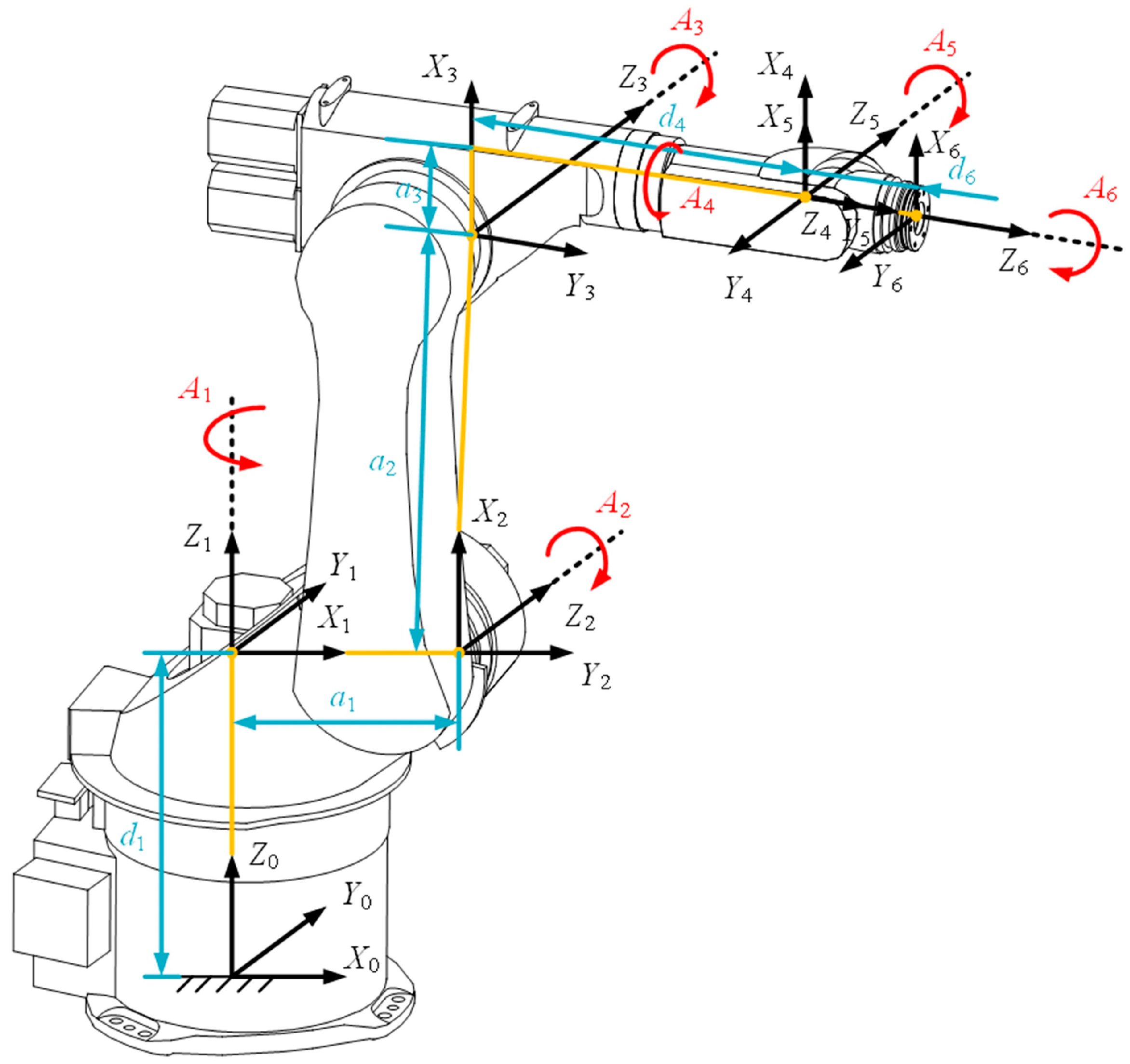
As shown in Figure 1, link frames based on the DHm model are established, numbered 0 to 6. Among them, the Frame 0 is the base frame, which origin is located at the robot base and is solidly connected to the ground as a reference frame to describe the poses of other joints of the robot. The DHm parameters of the KUKA KR60-3 robot are shown in Table 1. The link frames are defined as:

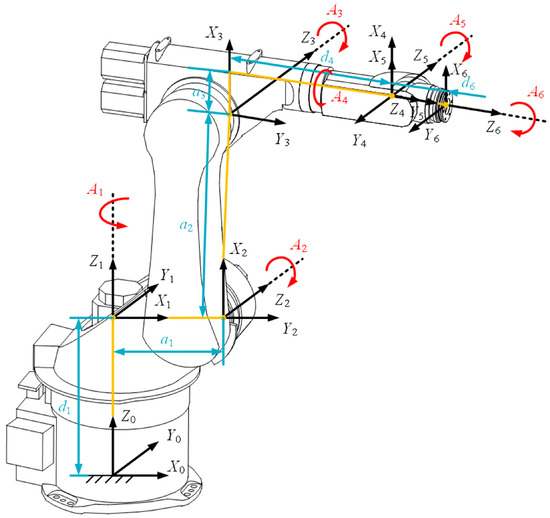
Figure 1. Link frames of KUKA KR60-3.

Table 1. DHm parameterization of KUKA KR60-3.

Link i	di/mm	ai−1/mm	ai−1/°
1	815	0	0
2	0	350	−90
3	0	850	0
4	820	145	−90
5	0	0	90
6	170	0	−90

(1)

${\mathit{A}}_i$ is axis $i$.

(2)

${\mathit{Z}}_i$ is along joint $i$, and the ${\mathit{X}}_i$ is along the common normal between ${\mathit{A}}_i$ and ${\mathit{A}}_{i-1}$. The choice of ${\mathit{X}}_i$ is not unique if the axes ${\mathit{Z}}_i$ and ${\mathit{Z}}_{i+1}$ are parallel. For convenience, direction from ${\mathit{A}}_i$ to ${\mathit{A}}_{i+1}$ is provided.

(3)

${\mathit{Y}}_i$ is chosen to form a right-handed coordinate system.

The Jacobian matrix $\mathit{J}$ of the robot describes the relationship between the end-effector linear and angular velocities and the joint velocities [27]. The differential kinematics equation is

$${\mathit{v}}_e=\left[\begin{array}{c}{\dot{\mathit{p}}}_e\\ {\mathit{\omega }}_e\end{array}\right]=\mathit{J}\left(\mathit{q}\right)\dot{\mathit{q}}$$

(1)

where Equation (1) expressed the end-effector linear velocity ${\dot{\mathit{p}}}_e$ and angular velocity ${\mathit{\omega }}_e$ as a function of the joint velocities $\dot{\mathit{q}}$. The $\left(6\times n\right)$ Jacobian matrix $\mathit{J}$ is the geometric Jacobian:

$$\mathit{J}=\left[\begin{array}{c}{\mathit{J}}_P\\ {\mathit{J}}_O\end{array}\right]$$

(2)

where ${\mathit{J}}_P$ and ${\mathit{J}}_O$ are the $\left(3\times n\right)$ matrices relating the contribution of $\dot{\mathit{q}}$ to ${\dot{\mathit{p}}}_e$ and ${\mathit{\omega }}_e$, respectively. Equation (2) is the joint variables’ function in general.

The $\left(3\times 1\right)$ column vectors ${\mathit{J}}_{Pi}$ and ${\mathit{J}}_{Oi}$ as follows can be used to divide the Jacobian:

$$\mathit{J}=\left[\begin{array}{ccc}{\mathit{J}}_{P1}& \cdots & {\mathit{J}}_{Pn}\\ ⋮& \ddots & ⋮\\ {\mathit{J}}_{O1}& \cdots & {\mathit{J}}_{On}\end{array}\right]$$

(3)

where

$$\left[\begin{array}{c}{\mathit{J}}_{Pi}\\ {\mathit{J}}_{Oi}\end{array}\right]=\{\begin{array}{c}\left[\begin{array}{c}{\mathit{z}}_{i-1}\\ \mathbf{0}\end{array}\right]\\ \left[\begin{array}{c}{\mathit{z}}_{i-1}\times \left({\mathit{p}}_e-{\mathit{p}}_{i-1}\right)\\ {\mathit{z}}_{i-1}\end{array}\right]\end{array}\begin{array}{c}\begin{array}{c}\mathrm{prismatic} \mathrm{joint}\\ \end{array}\\ \mathrm{revolute} \mathrm{joint}\end{array}$$

(4)

where ${\mathit{z}}_{i-1}$ is the unit vector of the joint $i$ axis.

Considering $n=6$, the Jacobian matrix can be divided into four $\left(3\times 3\right)$ matrix parts:

$$\mathit{J}=\left[\begin{array}{cc}{\mathit{J}}_{11}& {\mathit{J}}_{12}\\ {\mathit{J}}_{21}& {\mathit{J}}_{22}\end{array}\right]$$

(5)

where the expressions of the two right parts are as follows, respectively, since the outer three joints are revolute:

$${\mathit{J}}_{12}=\left[\begin{array}{ccc}{\mathit{z}}_3\times \left({\mathit{p}}_e-{\mathit{p}}_3\right)& {\mathit{z}}_4\times \left({\mathit{p}}_e-{\mathit{p}}_4\right)& {\mathit{z}}_5\times \left({\mathit{p}}_e-{\mathit{p}}_5\right)\end{array}\right]$$

(6)

$${\mathit{J}}_{22}=\left[\begin{array}{ccc}{\mathit{z}}_3& {\mathit{z}}_4& {\mathit{z}}_5\end{array}\right]$$

(7)

Singularities are irrelevant to the choice of the frames to describe the kinematics, which are dependent on the mechanical structure. Therefore, select the origin of the EE frame at the intersection of the wrist axes and choose $\mathit{p}={\mathit{p}}_w$ which leads to

$${\mathit{J}}_{12}=\left[\begin{array}{ccc}\mathbf{0}& \mathbf{0}& \mathbf{0}\end{array}\right]$$

(8)

For $i=3,4,5$, no matter how the frame is chosen, all vectors ${\mathit{p}}_w-{\mathit{p}}_i$ are parallel to the unit vector ${\mathit{z}}_i$. In this case, the global Jacobian matrix becomes a blocked lower triangular matrix:

$$\mathit{J}=\left[\begin{array}{cc}{\mathit{J}}_{11}& \mathbf{0}\\ {\mathit{J}}_{21}& {\mathit{J}}_{22}\end{array}\right]$$

(9)

The matrix determinant can be obtained by the multiplication of the determinants of the two parts on the diagonal:

$$\det \left(\mathit{J}\right)=\det \left({\mathit{J}}_{11}\right)\det \left({\mathit{J}}_{22}\right)$$

(10)

Accordingly, singularity decoupling can be achieved:

$$\{\begin{array}{c}\det \left({\mathit{J}}_{11}\right)=0\\ \det \left({\mathit{J}}_{22}\right)=0\end{array}\begin{array}{c}\mathrm{arm} \mathrm{singularities}\\ \mathrm{wrist} \mathrm{singularities}\end{array}$$

(11)

Therefore, the arm–wrist Jacobian matrix ${\mathit{J}}_{AW}={\mathit{J}}_{11}{\mathit{J}}_{22}$ is established to measure the dexterity of the robot.

2.2. Stiffness Modeling

The components of an industrial robot, including links and joints, are nonrigid and are subject to tensile, bending, and torsional deformations in the Cartesian workspace. The stiffness of an industrial robot is derived from the stiffness of the joints, links, and actuators, as well as the dynamic stiffness of the controller. The joints account for more than 70% of the overall deformation, including gear, timing belt, and motor transmission deformations. To simplify the calculations and not lose the generality, this paper assumes that the joint is a torsion spring, and the links are rigid bodies.

The relationship between the external forces and moments $\mathit{F}$ and the robot joint torques $\mathit{\tau }$:

$$\mathit{\tau }={\mathit{J}}^T\mathit{F}.$$

(12)

where ${\mathit{J}}^T$ is called the force Jacobian matrix, which is the transpose of the Jacobian matrix $\mathit{J}$; the six-dimensional vector $\mathit{F}$ represents the external forces and moments acting on the robot EE, and $\mathit{\tau }$ is related to the joint angle variation vector $\Delta \mathit{q}$:

$$\mathit{\tau }={\mathit{K}}_{\theta }\Delta \mathit{q}.$$

(13)

where ${\mathit{K}}_{\theta }$ is the stiffness matrix in the joint space, ${\mathit{K}}_{\theta }=diag\left(k_1,k_2,\dots ,k_6\right)$, and $k_i$ is the value of the ith joint stiffness. The relationship between deformation in the Cartesian space $\Delta \mathit{X}$ and $\mathit{F}$ is as follows:

$$\mathit{F}={\mathit{K}}_X\Delta \mathit{X}$$

(14)

where ${\mathit{K}}_X$ is the stiffness matrix in the Cartesian space.

The differentiation of Equation (12):

$$\frac{\partial \mathit{\tau }}{\partial \mathit{q}}=\left(\frac{\partial {\mathit{J}}^T}{\partial \mathit{q}}\right)\mathit{F}+{\mathit{J}}^T\frac{\partial \mathit{F}}{\partial \mathit{X}}\frac{\partial \mathit{X}}{\partial \mathit{q}}$$

(15)

$${\mathit{K}}_{\theta }={\mathit{K}}_C+{\mathit{J}}^T{\mathit{K}}_X\mathit{J}$$

(16)

where the complementary stiffness matrix (CoSM) ${\mathit{K}}_C$ can be expressed as the robot is subjected to external loading or the Jacobian changes with its configuration, and as long as the robot configurations are chosen appropriately, ${\mathit{K}}_C$ can be negligible. Thus, Equation (16) is simplified as:

$${\mathit{K}}_{\theta }={\mathit{J}}^T{\mathit{K}}_X\mathit{J}$$

(17)

The general form of the robot stiffness is shown in Equation (17). Once the robot configurations are chosen, we can get ${\mathit{K}}_X$ to obtain ${\mathit{K}}_{\theta }$ by Equation (17).

3. Method for Optimizing Robot Configuration

3.1. Optimize Robot Configuration Based on Kinematic Performance

${\mathit{J}}_{AW}$ is chosen as the criterion for optimizing the robot configuration. The Jacobian matrix condition number is widely used to measure the dexterity of the robot and the distance of the robot from the singularities. Therefore, the arm–wrist Jacobian matrix condition number is defined in terms of the Frobenius norm as follows:

$$\kappa \left({\mathit{J}}_{AW}\right)=\left|\right|{\mathit{J}}_{AW}|{|}_F=|\left|{\mathit{J}}_{11}\right|{|}_F\left|\right|{\mathit{J}}_{22}|{|}_F$$

(18)

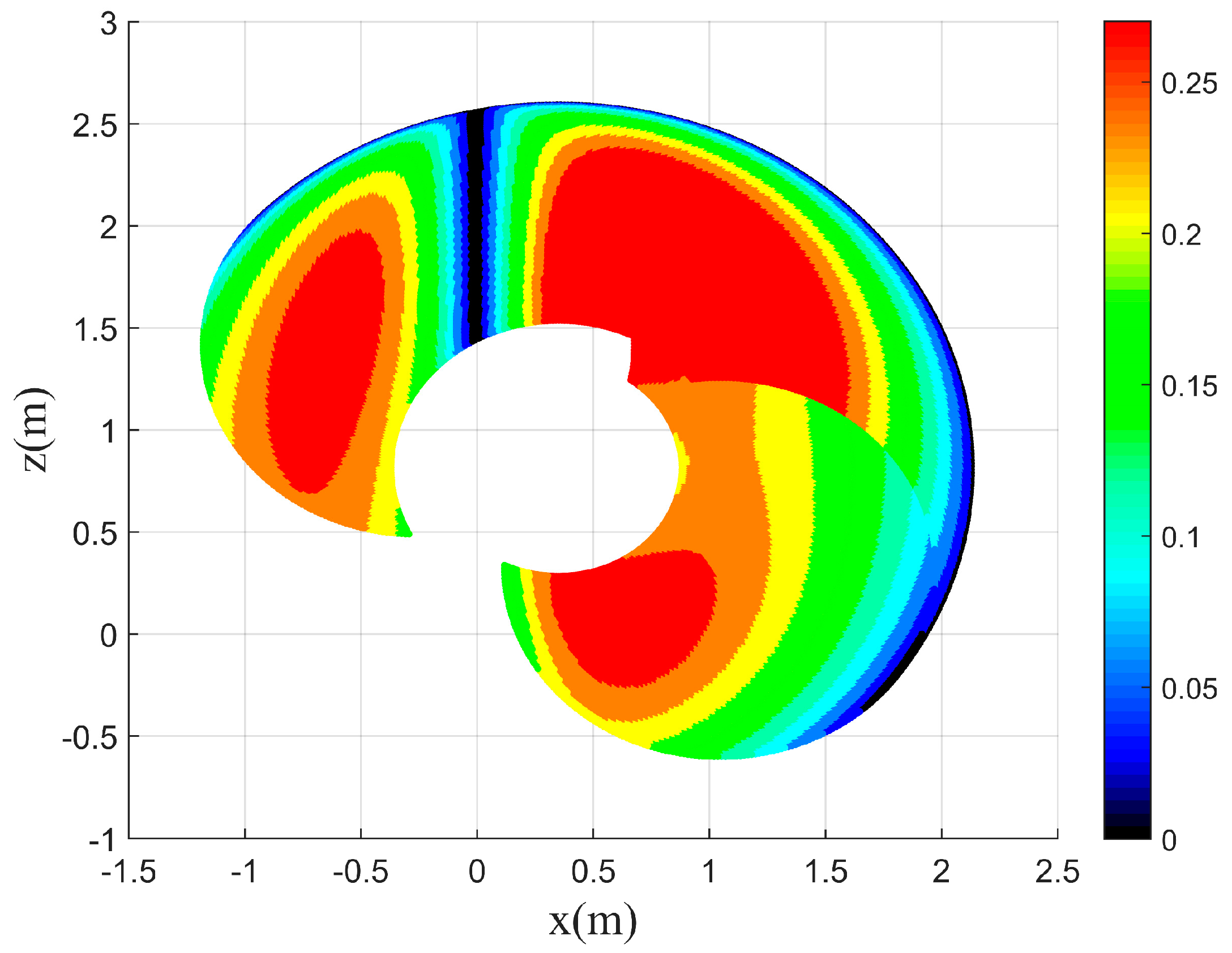
Figure 2 shows the contour drawing of $\kappa {\left({\mathit{J}}_{AW}\right)}^{-1}$ throughout the Cartesian workspace of the robot. The higher the $\kappa {\left({\mathit{J}}_{AW}\right)}^{-1}$ means the better the dexterity. The lower the $\kappa {\left({\mathit{J}}_{AW}\right)}^{-1}$ means the robot is closer to the singularities, which is the darker area in Figure 2. Since the first and sixth joints have no effect on $\kappa {\left({\mathit{J}}_{AW}\right)}^{-1}$, θ1 = 0° and θ6 = 45° are chosen to plot the contour drawing of $\kappa {\left({\mathit{J}}_{AW}\right)}^{-1}$ in the Cartesian workspace.

Figure 2. The contour drawing of $\kappa {\left({\mathit{J}}_{AW}\right)}^{-1}$.

There are four parameters, and they are independent of each other. The objective function is complex, and it is hard to obtain the derivation. Therefore, the maximum value of $\kappa {\left({\mathit{J}}_{AW}\right)}^{-1}$ in the Cartesian workspace is solved using the genetic algorithm

$$\begin{array}{l}\max f\left(x\right)=\kappa {\left({\mathit{J}}_{AW}\left(q_2,q_3,q_4,q_5\right)\right)}^{-1}\\ \{\begin{array}{l}{a}_1\le q_2\le a_2\\ b_1\le q_3\le b_2\\ c_1\le q_4\le c_2\\ d_1\le q_5\le d_2\\ \kappa \left({\mathit{J}}_{AW}\right)=\left|\right|{\mathit{J}}_{AW}|{|}_F=|\left|{\mathit{J}}_{11}\right|{|}_F\left|\right|{\mathit{J}}_{22}|{|}_F\end{array}\end{array}$$

(19)

where $q_i$ is the angle of the ith joint of the robot; $a_1$, $b_1$, $c_1$, and $d_1$ are the minimum values of the corresponding joint angles; and $a_2$, $b_2$, $c_2$, and $d_2$ are the maximum values of the corresponding joint angles, respectively.

Since the obtained optimal solutions for each group have similar influences and trends on $\kappa {\left({\mathit{J}}_{AW}\right)}^{-1}$, a set of $\kappa {\left({\mathit{J}}_{AW}\right)}^{-1}$ maximum poses with joint angles of [0° −4.4822° −99.912° 111.7901° 59.4099° 45°] were obtained to analyze the influence of each joint on $\kappa {\left({\mathit{J}}_{AW}\right)}^{-1}$.

3.2. The Influence of Each Joint on $\kappa {\left({\mathit{J}}_{AW}\right)}^{-1}$

To simplify the experimental procedure and reduce the parameters, it is important to analyze the degree of influence of each joint on $\kappa {\left({\mathit{J}}_{AW}\right)}^{-1}$.

Figure 3 shows the influence of the joint angle on $\kappa {\left({\mathit{J}}_{AW}\right)}^{-1}$ for joints 2, 3, 4, and 5 in their joint spaces.

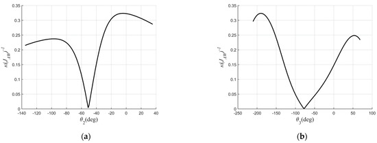
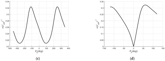
Figure 3. The influence of each joint on $\kappa {\left({\mathit{J}}_{AW}\right)}^{-1}$. (a) The influence of joint 2 on $\kappa {\left({\mathit{J}}_{AW}\right)}^{-1}$. (b) The influence of joint 3 on $\kappa {\left({\mathit{J}}_{AW}\right)}^{-1}$. (c) The influence of joint 4 on $\kappa {\left({\mathit{J}}_{AW}\right)}^{-1}$. (d) The influence of joint 5 on $\kappa {\left({\mathit{J}}_{AW}\right)}^{-1}$.

As shown in Figure 3, $\kappa {\left({\mathit{J}}_{AW}\right)}^{-1}=0$ means a singularity, and the maximum value of $\kappa {\left({\mathit{J}}_{AW}\right)}^{-1}$ is the pose mentioned above. The value of $\kappa {\left({\mathit{J}}_{AW}\right)}^{-1}$ represents the distance from the singularity. The larger the value of $\kappa {\left({\mathit{J}}_{AW}\right)}^{-1}$, the further the distance from the singularity and the better the dexterity of the joint. The rotation range of joint 4 exceeded 360 degrees, so there were two maximum values of $\kappa {\left({\mathit{J}}_{AW}\right)}^{-1}$.

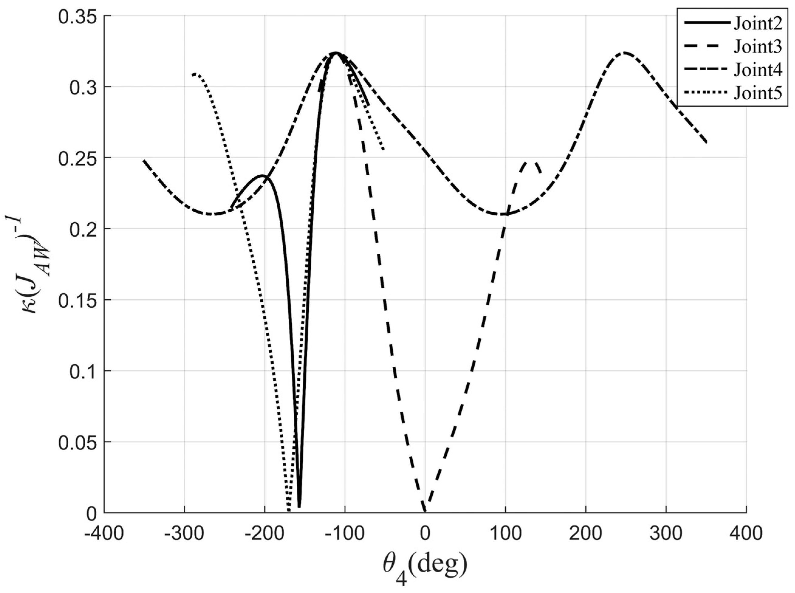
To visually see the influence of each joint on $\kappa {\left({\mathit{J}}_{AW}\right)}^{-1}$, the maximum dexterity pose of $\kappa {\left({\mathit{J}}_{AW}\right)}^{-1}$ of each joint mentioned above is panned out to the same point (based on the 4th joint space), and Figure 4 shows the value of $\kappa {\left({\mathit{J}}_{AW}\right)}^{-1}$ of each joint in the 4th joint space, and the larger the rate of change is (smaller the degree of opening) of the curve at the maximum (corresponding joints), the greater the influence is on $\kappa {\left({\mathit{J}}_{AW}\right)}^{-1}$.

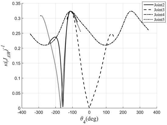
Figure 4. The influence of each joint on $\kappa {\left({\mathit{J}}_{AW}\right)}^{-1}$ in the 4th joint space.

In Figure 4, it is quite obvious that the rate of change of joint 4 is the smallest, i.e., the degree of influence is the smallest, but the rate of change of joints 2, 3, and 5 cannot be visually seen, so it is necessary to obtain the second derivative of each curve to find the rate of change of each joint at the maximum value, and a larger absolute value indicates a greater degree of influence. Perform eighth-order Fourier fitting on each curve to obtain the rate of change of each joint.

The degree of influence of each joint on $\kappa {\left({\mathit{J}}_{AW}\right)}^{-1}$ joints 5 > 2 > 3 > 4, as shown in Table 2.

Table 2. The rate of change of each joint at the maximum value of $\kappa {\left({\mathit{J}}_{AW}\right)}^{-1}$.

Joint Number	Joint 2	Joint 3	Joint 4	Joint 5
The rate of change	1.4172 × 10−4	−1.0774 × 10−4	−3.6893 × 10−5	−1.5070 × 10−4

3.3. Optimize Robot Configuration in 2nd and 3rd Joint Space

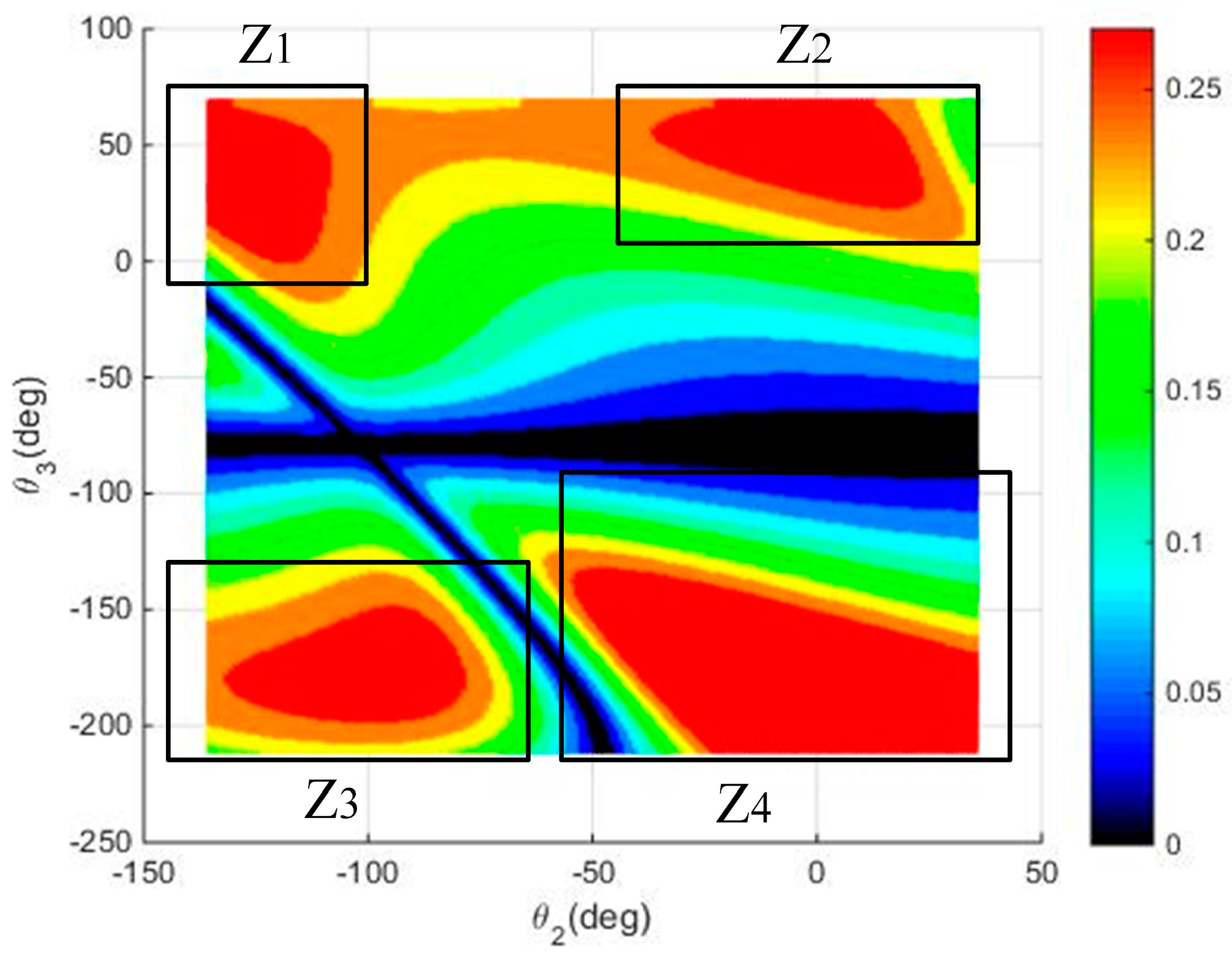
As can be seen from Table 2, joints 2 and 5 have a similar degree of influence, and it is necessary to choose a continuous joint space for simplifying the experiment, and joints 2 and 3 are the joints with the greatest influence on the end Cartesian space position, so joints 2 and 3 are chosen to plot the contour drawing of $\kappa {\left({\mathit{J}}_{AW}\right)}^{-1}$.

Figure 5 shows the contour drawing of $\kappa {\left({\mathit{J}}_{AW}\right)}^{-1}$ in the 2 and 3 joint spaces. It can be seen that there are four areas where larger $\kappa {\left({\mathit{J}}_{AW}\right)}^{-1}$ values can be obtained (far from the singularities). The Z₂ area cannot be selected because of the limitation of the experimental space (the robot pose in this area cannot be reached in the laboratory), and the Z₃ area cannot be selected because the end of the robot is too close to the ground, so it is hard to measure. Therefore, the Z₁ and Z₄ areas are selected as the poses to identify the joint stiffness of the robot.

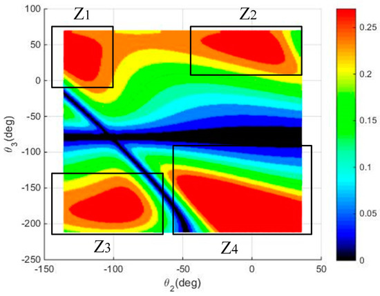
Figure 5. Contour drawing of $\kappa {\left({\mathit{J}}_{AW}\right)}^{-1}$ in the 2 and 3 joint spaces.

4. Method for the Joint Stiffness Identification

4.1. Joint Stiffness Identification

From Equation (17), the external forces and moments $\mathit{F}$ can be written as

$$\mathit{F}={\mathit{J}}^{-T}{\mathit{K}}_{\theta }{\mathit{J}}^{-1}\delta \mathit{d}$$

(20)

Thus, the robot EE displacement $\delta \mathit{d}$ is

$$\delta \mathit{d}=\mathit{J}{\mathit{K}}_{\theta }^{-1}{\mathit{J}}^T\mathit{F}$$

(21)

Let the joint compliances be the vector $\mathit{c}$

$$\mathit{c}={\left[\begin{array}{cc}\begin{array}{ccc}\frac{1}{k_{{\theta }_1}}& \frac{1}{k_{{\theta }_2}}& \frac{1}{k_{{\theta }_3}}\end{array}& \begin{array}{ccc}\frac{1}{k_{{\theta }_4}}& \frac{1}{k_{{\theta }_5}}& \frac{1}{k_{{\theta }_6}}\end{array}\end{array}\right]}^T$$

(22)

Equation (17) can be written as

$$\delta \mathit{d}=\left[\begin{array}{c}{\displaystyle {\sum }_{j=1}^6\left({\mathit{c}}_j{\mathit{J}}_{1j}{\displaystyle {\sum }_{i=1}^6{\mathit{J}}_{ij}{\mathit{F}}_i}\right)}\\ ⋮\\ {\displaystyle {\sum }_{j=1}^6\left({\mathit{c}}_j{\mathit{J}}_{6j}{\displaystyle {\sum }_{i=1}^6{\mathit{J}}_{ij}{\mathit{F}}_i}\right)}\end{array}\right]$$

(23)

where ${\mathit{F}}_j$ is the jth component of $\mathit{F}$ and ${\mathit{c}}_j$ is the jth component of $\mathit{c}$.

Isolating vector $\mathit{c}$ of Equation (23) is as follows:

$$\delta \mathit{d}=\mathit{Ac}$$

(24)

where $\mathit{A}$ is a $6\times 6$ matrix 22, namely

$$\mathit{A}=\left[\begin{array}{ccc}{\mathit{J}}_{11}{\displaystyle {\sum }_{i=1}^6{\mathit{J}}_{i1}{\mathit{F}}_i}& \cdots & {\mathit{J}}_{16}{\displaystyle {\sum }_{i=1}^6{\mathit{J}}_{i6}{\mathit{F}}_i}\\ ⋮& \ddots & ⋮\\ {\mathit{J}}_{61}{\displaystyle {\sum }_{i=1}^6{\mathit{J}}_{i1}{\mathit{F}}_i}& \cdots & {\mathit{J}}_{66}{\displaystyle {\sum }_{i=1}^6{\mathit{J}}_{i6}{\mathit{F}}_i}\end{array}\right]$$

(25)

4.2. Method for Obtaining the Robot EE Displacement

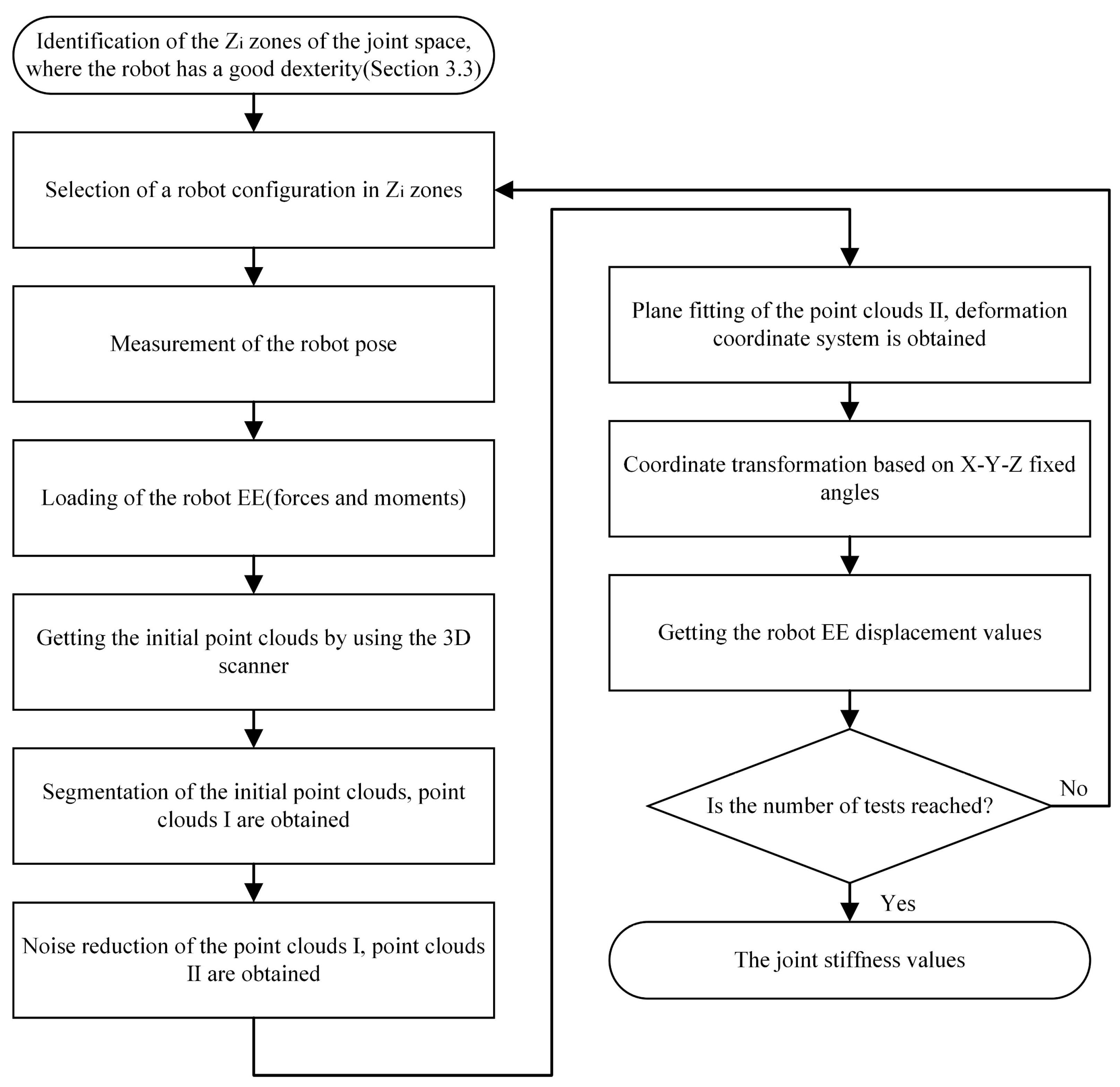
The joint stiffness identification procedure is shown in Figure 6. First, a robot configuration with good dexterity based on $\kappa {\left({\mathit{J}}_{AW}\right)}^{-1}$ is selected. Then, the robot EE displacement values are obtained by the procedure for point cloud processing. Eventually, the values of the joint stiffness are obtained when the number of tests is reached.

Figure 6. Procedure for the joint stiffness identification.

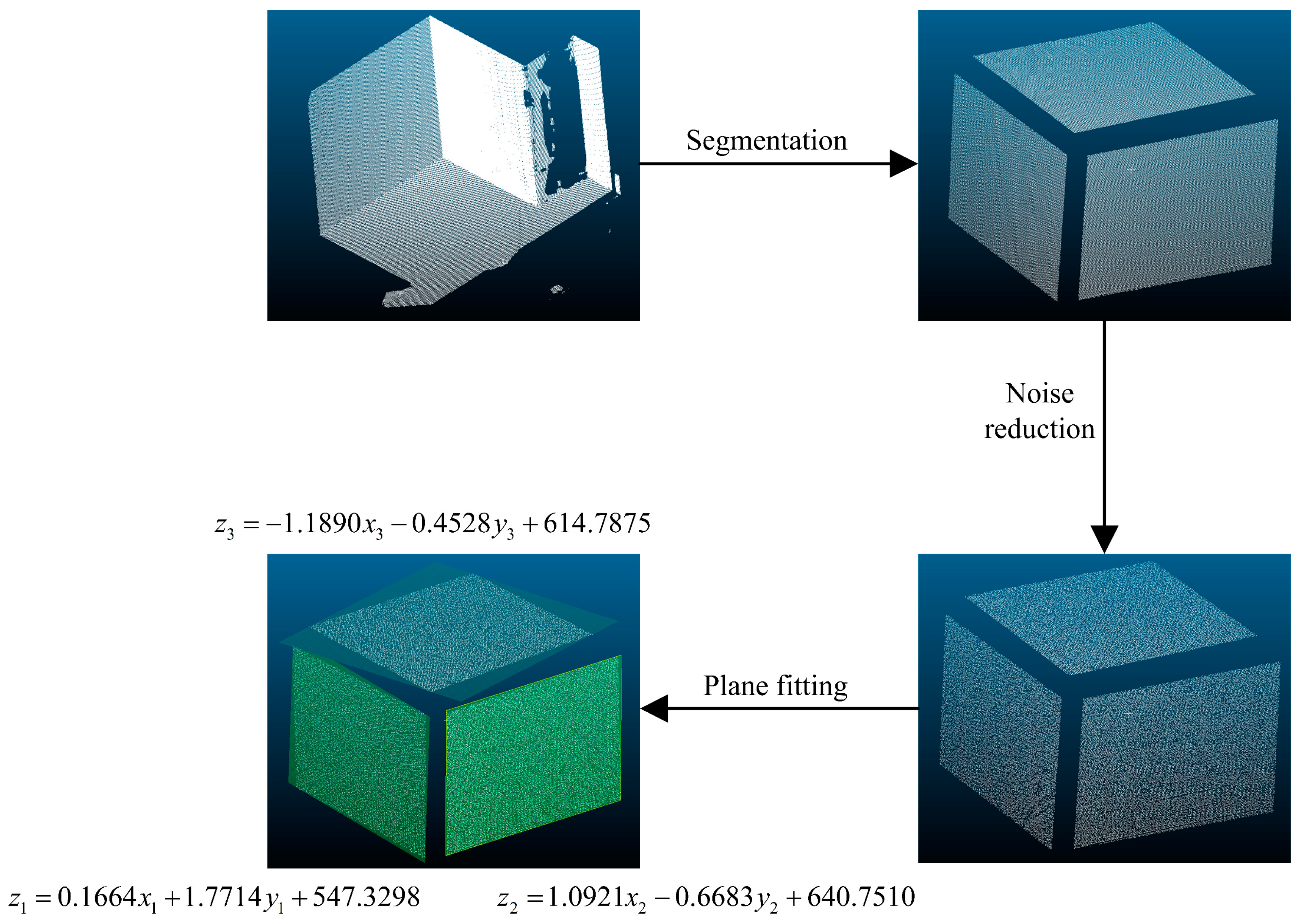
The measurement of the robot EE displacement is obtained by the EE target block displacement. The 3D scanner is used to obtain high-precision initial 3D point clouds of the surface of the target block at the end of the robot. The initial 3D point clouds need to be fitted to obtain the expression for the point cloud planes to set up the deformation coordinate system. The 3D point clouds usually contain noise points that will affect the accuracy of the deformation coordinate system. The processing of 3D point cloud data mainly includes segmentation, noise reduction, and plane fitting of the point clouds. The segmentation processing of the point clouds obtains three mutually vertical planar point clouds of YOZ, XOZ, and XOY. The noise reduction processing is to remove the noise points in the 3D point clouds. The plane fitting processing obtains the expressions of the point cloud planes. One experiment for an illustrative example was chosen to describe the procedure for obtaining the EE displacement (see Figure 7). z₁, z₂, and z₃ represent the fitted YOZ, XOZ, and XOY plane equations of the target block, respectively.

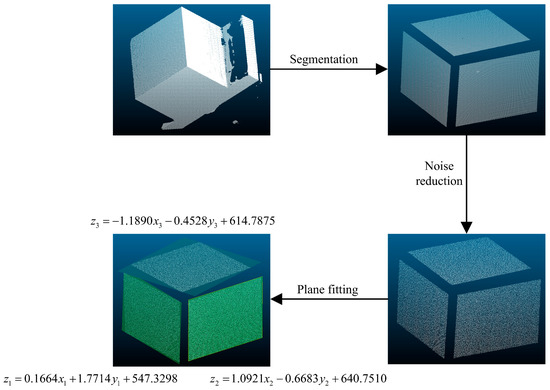
Figure 7. Procedure for obtaining the EE displacement.

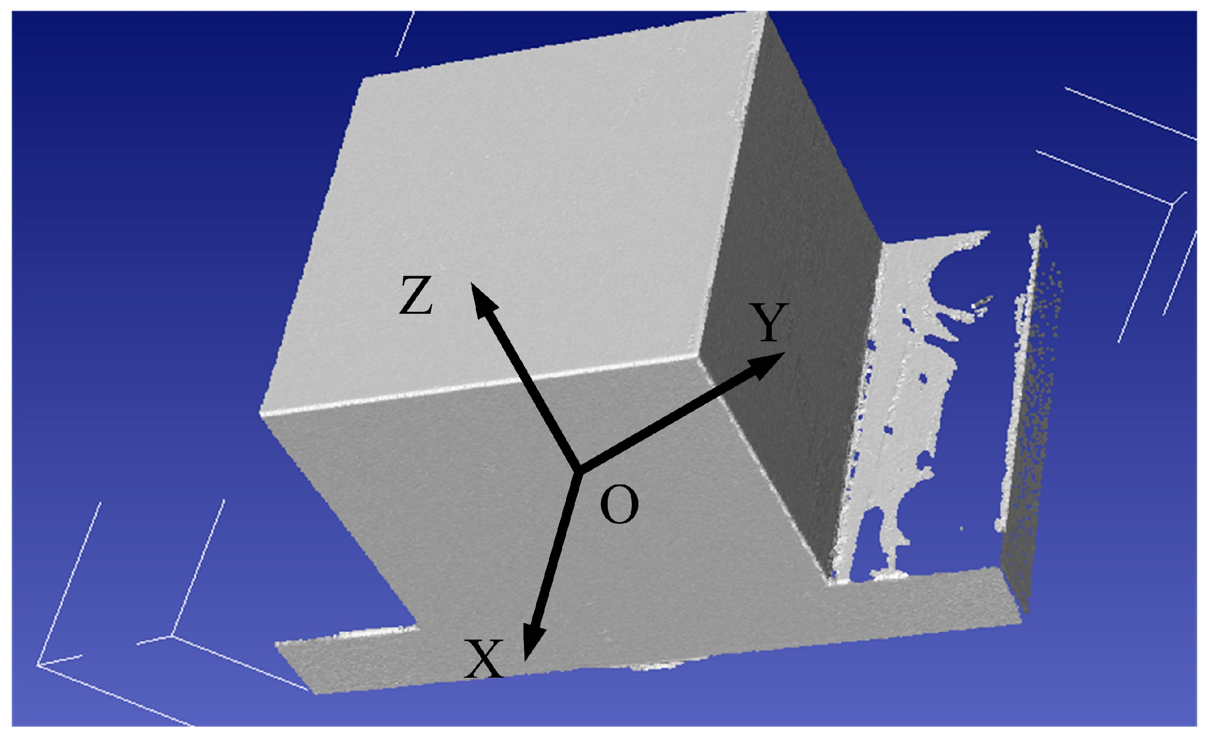
As shown in Figure 8, the coordinate system of the target block is established. Based on the normal vectors of the fitted YOZ, XOZ, and XOY planes and the intersection of the three planes as the origin, the deformation coordinate system is established:

$${\mathit{O}}_i=\left[\begin{array}{cccc}{a}_{i1}& a_{i2}& a_{i3}& o_{iox}\\ b_{i1}& b_{i2}& b_{i3}& o_{ioy}\\ c_{i1}& c_{i2}& c_{i3}& o_{ioz}\\ 0& 0& 0& 1\end{array}\right]$$

(26)

where $i=0$ means the deformation coordinate system before loading; $i=1$ means the deformation coordinate system after loading; $a$, $b$, and $c$ represent the plane normal vectors; and $o$ indicates the intersection point (origin) of the three planes.

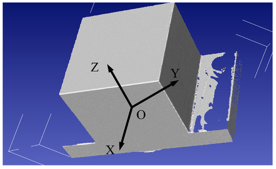
Figure 8. The target block at the end of the robot.

The transformation matrix $\mathit{T}$ from ${\mathit{O}}_0$ to ${\mathit{O}}_1$ is

$$\mathit{T}={\mathit{O}}_1{\mathit{O}}_0^{-1}=\left[\begin{array}{cc}\mathit{R}& \mathit{P}\\ \mathbf{0}& \mathbf{1}\end{array}\right]$$

(27)

where

$$\mathit{P}={\left[\begin{array}{ccc}dx& dy& dz\end{array}\right]}^T$$

(28)

$$\mathit{R}\left(\gamma ,\beta ,\alpha \right)=\left[\begin{array}{ccc}{r}_{11}& r_{12}& r_{13}\\ r_{21}& r_{22}& r_{23}\\ r_{31}& r_{32}& r_{33}\end{array}\right]$$

(29)

The two-argument arc tangent function Atan2 is used to obtain the rotation angles ($\gamma$, $\beta$, and $\alpha$) of coordinate axes $x$, $y$, and $z$:

$$\mathit{P}=\{\begin{array}{l}\gamma =A\tan 2\left(r_{32}/\cos \beta ,r_{33}/\cos \beta \right)\\ \beta =A\tan 2\left(-r_{31},\sqrt{r_{11}^2+r_{21}^2}\right)\\ \alpha =A\tan 2\left(r_{21}/\cos \beta ,r_{11}/\cos \beta \right)\end{array}$$

(30)

The robot EE deformation is obtained as follows:

$$\delta \mathit{d}={\left[\begin{array}{cc}\begin{array}{ccc}dx& dy& dz\end{array}& \begin{array}{ccc}\gamma & \beta & \alpha \end{array}\end{array}\right]}^T$$

(31)

5. Experiment Procedure

5.1. Experiment System

In Figure 9, the experimental system consists of a robot, a 3D scanner, a six-dimensional force sensor, a rotating ring, and a target block. The workspace radius of the KUKA KR60-3 robot is equal to 2033 mm, and the repeatability is ±0.06 mm. The force sensor and target block are rigidly attached to the robot flange. The measurement system must ensure fast and accurate measurements of multiple poses in the Cartesian workspace, for which a 3D scanner VTOP 200B from TECHLEGO (TIANJIN) CO., LTD was used. The parameters of the 3D scanner are shown in Table 3.

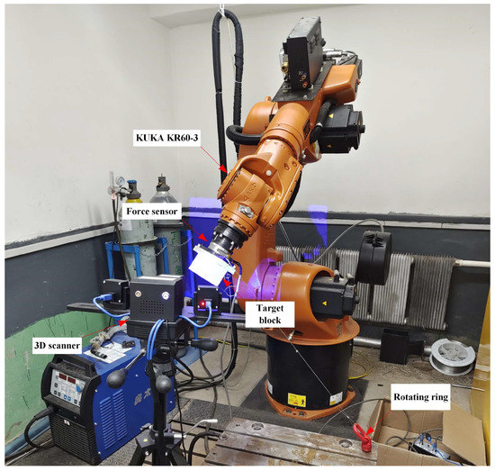
Figure 9. Experimental setup.

Table 3. Three-dimensional scanner VTOP 200B parameters.

Scanning Parameters	VTOP 200B
Scanning mode	Noncontact surface scanning
Resolution (pixels)	5 million, monochrome
Scanning accuracy (mm)	0.01–0.015
Scanning distance (mm)	100–1250
Measuring point distance (mm)	0.02–0.5
Measuring area (mm2)	50 × 38–450 × 342

The target block is connected to the rotating ring on the table by means of a high-strength steel wire. The end load of the robot is adjusted by the threaded fastening of the rotating ring to the table.

The robot EE deformation $\delta \mathit{d}$ is obtained from the 3D scanner, and the external forces and moments $\mathit{F}$ are measured by a six-dimensional force sensor (ATI DELTA SI-330-30), as shown in Table 4. $\delta \mathit{d}$ and $\mathit{F}$ are transformed into the robot EE coordinate system to gain $\mathit{c}$. Finally, the robot joint stiffness matrix ${\mathit{K}}_{\theta }$ is obtained.

Table 4. ATI force sensor parameters.

Axes	SI-330-30
Fx, Fy (±N)	330
Fz (±N)	990
Tx, Ty (±Nm)	30
Tz (±Nm)	30

5.2. Robustness of the Method

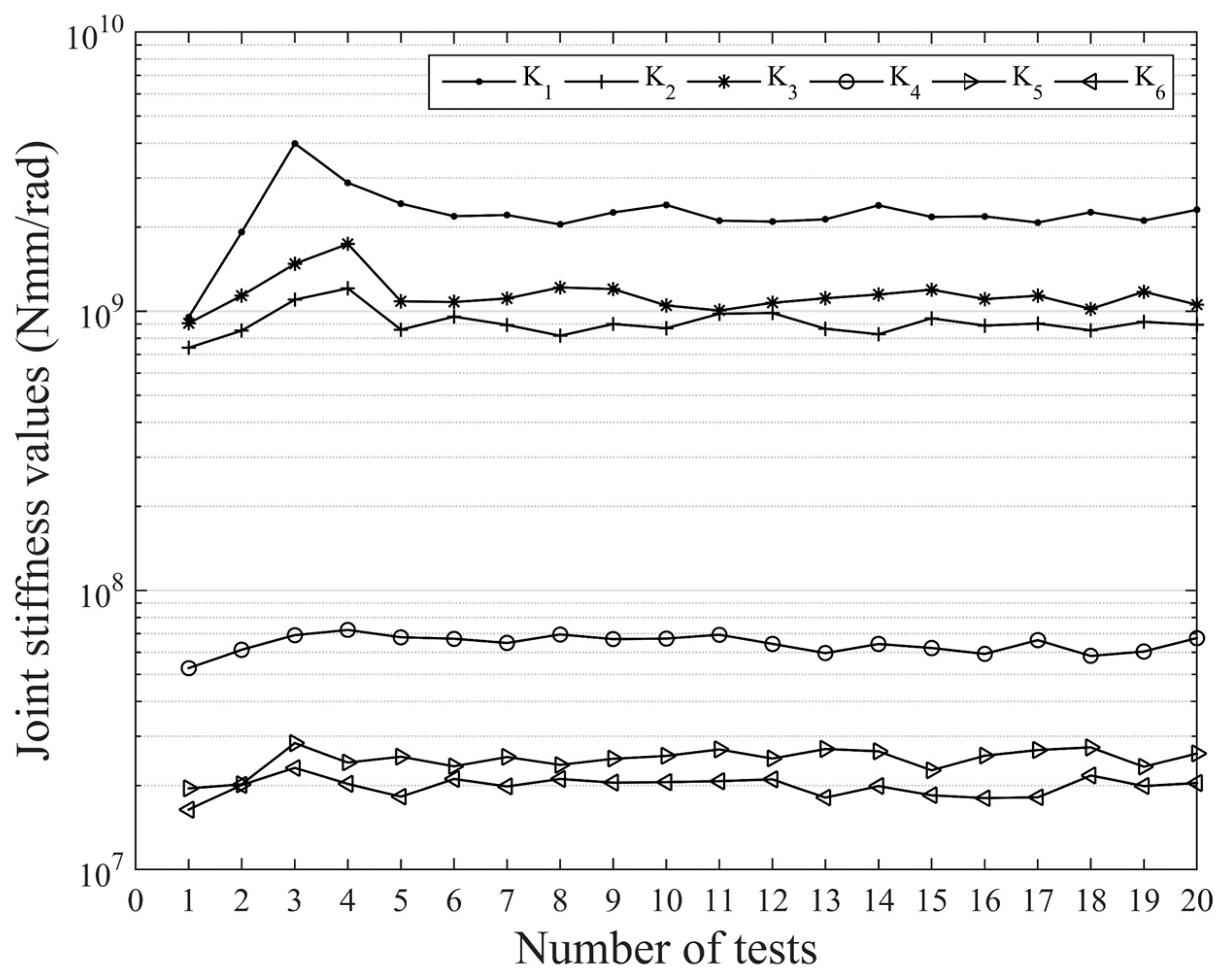
According to Equation (25), the Jacobian matrix $\mathit{J}$ can be obtained for a specific robot configuration, and the $6\times 6$ matrix $\mathit{A}$ can be obtained when the external forces and moments $\mathit{F}$ are measured by a six-dimensional force sensor. The robot EE deformation $\delta \mathit{d}$ can be obtained by the method in Section 4.2. Therefore, to analyze the robustness of the method, ${\mathit{K}}_{\theta }$ can be obtained by Equation (24) with one test. As shown in Figure 10, the joint stiffnesses $k_{{\theta }_1}$, $k_{{\theta }_2}$, $k_{{\theta }_3}$, $k_{{\theta }_4}$, $k_{{\theta }_5}$, and $k_{{\theta }_6}$ were obtained by the method for $n$ tests, $n=1,2,\dots ,20$. Twenty groups of tests were randomly selected. The convergence of joint stiffness values becomes better as the number of tests increases and the results are more reliable. When the number of tests is higher than five, the joint stiffness identification method is considered to be robust.

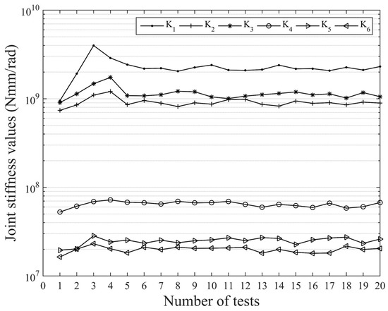
Figure 10. Robustness of the tests.

Therefore, the 6th–20th group of tests was selected for analysis. The values of the joint stiffness were fitted using the least squares method, and the joint stiffness values, error ranges, and mean errors are shown in Table 5.

Table 5. The values and errors of joint stiffness.

Joint Number	Stiffness Values (Nmm/rad)	Error Ranges in (%)	Mean Errors in (%)
1	2.1977 × 109	−6.97~9.42	−0.30
2	8.9939 × 108	−3.75~3.91	0.02
3	1.1118 × 109	−4.82~4.76	0.33
4	6.4449 × 107	−0.28~0.23	−0.29
5	2.5362 × 107	−0.12~0.09	−0.19
6	1.9978 × 107	−0.09~0.08	−0.19

As shown in Table 5, the experimental errors are within ±10%, and the mean errors are within ±0.5%. The reason for the larger errors in joints 1, 2, and 3 is that the joint stiffness values are larger, resulting in smaller displacements in their joint space and lower measurement accuracy. Therefore, the experiment is reliable and stable for the identification of robot joint stiffness due to the relatively small errors and mean errors.

5.3. Error Analysis

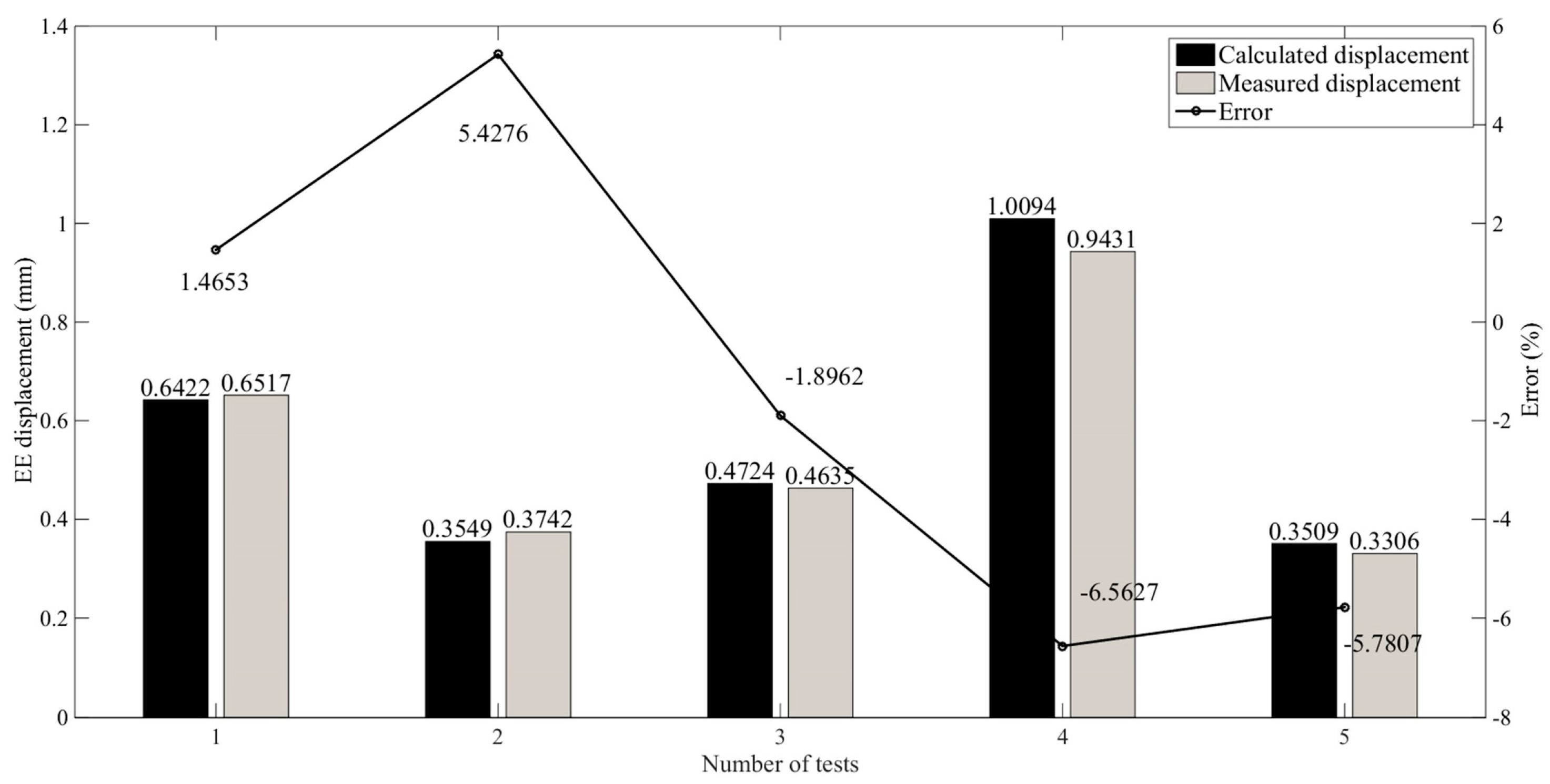
The robot configuration for validation experiments is shown in Table 6. The calculated and measured EE displacements are shown in Figure 11. The validation is realized by a random set of five poses in the Cartesian workspace. The calculated EE displacement is indicated by dark-colored bars, and the measured EE displacement is indicated by light-colored bars. The line indicates the relative error of the two displacements. The errors are less than 10%, which proves that the calculated displacement values are close to the measured displacement values. Therefore, the joint stiffness identification method is feasible.

Table 6. Robot configuration for the validation experiments.

Number of Tests	θ1 (Deg)	θ2 (Deg)	θ3 (Deg)	θ4 (Deg)	θ5 (Deg)	θ6 (Deg)
1	−2.09	−99.89	149.24	172.57	56.97	−189.47
2	−1.87	−102.59	117.78	98.36	−85.67	−152.43
3	13.57	−98.15	115.69	250.37	−24.18	−159.38
4	−3.68	−22.43	48.14	74.26	−58.51	−102.47
5	−1.54	−77.52	86.33	96.81	−84.01	−147.35

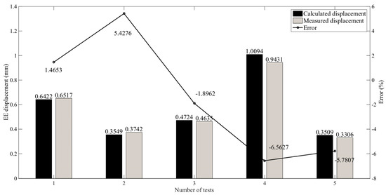
Figure 11. Calculated and measured displacements of the EE and the percentage of error.

6. Conclusions

In this paper, a new robot joint stiffness identification method is proposed. The method considers the coupling of translational and rotational displacements of the EE, and it is convenient to identify the robot joint stiffness values. The KUKA KR60-3 robot is used as a representative example in this paper. First, the kinematic performance model of the robot is obtained, and the optimal pose of the robot is determined according to the kinematic arm–wrist Jacobian matrix condition number $\kappa {\left({\mathit{J}}_{AW}\right)}^{-1}$. Then, the influence of each joint on $\kappa {\left({\mathit{J}}_{AW}\right)}^{-1}$ is analyzed, and the corresponding joint is selected to simplify the experiment. Next, the stiffness model is established, and the joint stiffness matrix ${\mathit{K}}_{\theta }$ and good stability of the experiment are obtained. Finally, the experimental errors are analyzed, and the experimental errors are within 10%, which are able to obtain an approximation of the real joint stiffness values and provide a good basis for subsequent robot machining with this stiffness model. In future work, the link stiffness will be considered to complete the joint stiffness identification method, and the complementary stiffness matrix (CoSM) will also be analyzed for its effect on the identification of the robot joint stiffness.

References

- Bi, S.; Liang, J. Robotic drilling system for titanium structures. Int. J. Adv. Manuf. Technol. 2010, 54, 767–774. [Google Scholar] [CrossRef]
- Zhu, W.; Qu, W.; Cao, L.; Yang, D.; Ke, Y. An off-line programming system for robotic drilling in aerospace manufacturing. Int. J. Adv. Manuf. Technol. 2013, 68, 2535–2545. [Google Scholar] [CrossRef]
- Saravanan, R.; Ramabalan, S.; Balamurugan, C. Evolutionary optimal trajectory planning for industrial robot with payload constraints. Int. J. Adv. Manuf. Technol. 2007, 38, 1213–1226. [Google Scholar] [CrossRef]
- Zheng, H.D.; Cong, M.; Dong, H.; Liu, Y.; Liu, D. CAD-based automatic path generation and optimization for laser cladding robot in additive manufacturing. Int. J. Adv. Manuf. Technol. 2017, 92, 3605–3614. [Google Scholar] [CrossRef]
- Mattmüller, J.; Gisler, D. Calculating a near time-optimal jerk-constrained trajectory along a specified smooth path. Int. J. Adv. Manuf. Technol. 2009, 45, 1007–1016. [Google Scholar] [CrossRef]
- Zha, X.F. Optimal pose trajectory planning for robot manipulators. Mech. Mach. Theory 2002, 37, 1063–1086. [Google Scholar] [CrossRef]
- Tian, Y.; Wang, B.; Liu, J.; Chen, F.; Yang, S.; Wang, W.; Li, L. Research on layout and operational pose optimization of robot grinding system based on optimal stiffness performance. J. Adv. Mech. Des. Syst. Manuf. 2017, 11, JAMDSM0022. [Google Scholar] [CrossRef]
- Dumas, C.; Caro, S.; Garnier, S.; Furet, B. Joint stiffness identification of six-revolute industrial serial robots. Robot. Comput. Manuf. 2011, 27, 881–888. [Google Scholar] [CrossRef]
- Bu, Y.; Liao, W.; Tian, W.; Zhang, L.; Dawei, L. Modeling and experimental investigation of Cartesian compliance characterization for drilling robot. Int. J. Adv. Manuf. Technol. 2017, 91, 3253–3264. [Google Scholar] [CrossRef]
- Bu, Y.; Liao, W.; Tian, W.; Zhang, J.; Zhang, L. Stiffness analysis and optimization in robotic drilling application. Precis. Eng. 2017, 49, 388–400. [Google Scholar] [CrossRef]
- Guerin, D.; Caro, S.; Garnier, S.; Girin, A. Optimal Measurement Pose Selection f-or Joint Stiffness Identification of an Industrial Robot Mounted on a Rail. In Proceedings of the 2014 IEEE/ASME International Conference on Advanced Intelligent Mechatronics, Besacon, France, 8–11 July 2014; pp. 1722–1727. [Google Scholar]
- Xiong, G.; Ding, Y.; Zhu, L. Stiffness-based pose optimization of an industrial robot for five-axis milling. Robot. Comput. Manuf. 2018, 55, 19–28. [Google Scholar] [CrossRef]
- Chen, C.; Peng, F.; Yan, R.; Li, Y.; Wei, D.; Fan, Z.; Tang, X.; Zhu, Z. Stiffness performance index based posture and feed orientation optimization in robotic milling process. Robot. Comput. Manuf. 2018, 55, 29–40. [Google Scholar] [CrossRef]
- Kucuk, S.; Bingul, Z. Comparative study of performance indices for fundamental robot manipulators. Robot. Auton. Syst. 2006, 54, 567–573. [Google Scholar] [CrossRef]
- Pan, Z.; Zhang, H. Analysis and suppression of chatter in robotic machining process. In Proceedings of the 2007 International Conference on Control, Automation and Systems, Seoul, Republic of Korea, 17–20 October 2007; pp. 2874–2879. [Google Scholar]
- Matsuoka, S.-I.; Shimizu, K.; Yamazaki, N.; Oki, Y. High-speed end milling of an articulated robot and its characteristics. J. Mater. Process. Technol. 1999, 95, 83–89. [Google Scholar] [CrossRef]
- Pan, Z.; Zhang, H.; Zhu, Z.; Wang, J. Chatter analysis of robotic machining process. J. Mater. Process. Technol. 2006, 173, 301–309. [Google Scholar] [CrossRef]
- Liao, Z.-Y.; Li, J.-R.; Xie, H.-L.; Wang, Q.-H.; Zhou, X.-F. Region-based toolpath generation for robotic milling of freeform surfaces with stiffness optimization. Robot. Comput. Manuf. 2020, 64, 101953. [Google Scholar] [CrossRef]
- Denkena, B.; Lepper, T. Enabling an Industrial Robot for Metal Cutting Operations. Procedia CIRP 2015, 35, 79–84. [Google Scholar] [CrossRef]
- Alici, G.; Shirinzadeh, B. Enhanced stiffness modeling, identification and characterization for robot manipulators. IEEE Trans. Robot. 2005, 21, 554–564. [Google Scholar] [CrossRef]
- Chen, S.-F.; Kao, I. Conservative Congruence Transformation for Joint and Cartesian Stiffness Matrices of Robotic Hands and Fingers. Int. J. Robot. Res. 2000, 19, 835–847. [Google Scholar] [CrossRef]
- Dumas, C.; Caro, S.; Cherif, M.; Garnier, S.; Furet, B. Joint stiffness identification of industrial serial robots. Robotica 2011, 30, 649–659. [Google Scholar] [CrossRef]
- Cvitanic, T.; Nguyen, V.; Melkote, S.N. Pose optimization in robotic machining using static and dynamic stiffness models. Robot. Comput. Manuf. 2020, 66, 101992. [Google Scholar] [CrossRef]
- Li, G.; Zhu, W.; Dong, H.; Ke, Y. Stiffness-oriented performance indices defined on two-dimensional manifold for 6-DOF industrial robot. Robot. Comput. Manuf. 2020, 68, 102076. [Google Scholar] [CrossRef]
- Guo, Y.; Dong, H.; Ke, Y. Stiffness-oriented posture optimization in robotic machining applications. Robot. Comput. Manuf. 2015, 35, 69–76. [Google Scholar] [CrossRef]
- Cen, L.; Melkote, S.N. CCT-based mode coupling chatter avoidance in robotic milling. J. Manuf. Process. 2017, 29, 50–61. [Google Scholar] [CrossRef]
- Siciliano, B.; Sciavicco, L.; Villani, L.; Oriolo, G. Differential Kinematics and Statics. In Robotics: Modelling, Planning and Control; Springer: London, UK, 2009; pp. 105–160. [Google Scholar] [CrossRef]
Disclaimer/Publisher’s Note: The statements, opinions and data contained in all publications are solely those of the individual author(s) and contributor(s) and not of MDPI and/or the editor(s). MDPI and/or the editor(s) disclaim responsibility for any injury to people or property resulting from any ideas, methods, instructions or products referred to in the content. |
© 2023 by the authors. Licensee MDPI, Basel, Switzerland. This article is an open access article distributed under the terms and conditions of the Creative Commons Attribution (CC BY) license (https://creativecommons.org/licenses/by/4.0/).