Fused Node-Level Residual Structure Edge Graph Neural Network for Few-Shot Image Classification

Abstract

In spite of recent rapid developments across various computer vision domains, numerous cutting-edge deep learning algorithms often demand a substantial volume of data to operate effectively. Within this research, a novel few-shot learning approach is presented with the objective of enhancing the accuracy of few-shot image classification. This task entails the classification of unlabeled query samples based on a limited set of labeled support examples. Specifically, the integration of the edge-conditioned graph neural network (EGNN) framework with hierarchical node residual connections is proposed. The primary aim is to enhance the performance of graph neural networks when applied to few-shot classification, a rather unconventional application of hierarchical node residual structures in few-shot image classification tasks. It is noteworthy that this work represents an innovative attempt to combine these two techniques. Extensive experimental findings on publicly available datasets demonstrate that the methodology surpasses the original EGNN algorithm, achieving a maximum improvement of 2.7%. Particularly significant is the performance gain observed on our custom-built dataset, CBAC (Car Brand Appearance Classification), which consistently outperforms the original method, reaching an impressive peak improvement of 11.14%.

1. Introduction

Deep learning has shown to be quite successful in tackling complicated challenges in the current digital era. However, a sizable amount of labeled training data is often required [1,2]. Humans, on the other hand, have the amazing capacity to learn quickly from a little amount of material. Few-Shot Learning (FSL) is a concept that was developed in response to how people learn. It seeks to construct models that can perform well even with little labeled data or in situations when there is little data available.

Due to this, both the academic and corporate worlds have shifted their attention in recent years to the area of “few-shot classification”. The difficulty of learning and using new categories or concepts when there is a severe lack of training data is addressed in this field [3,4,5,6,7,8,9,10]. Researchers have begun to investigate techniques for few-shot picture categorization in the context of deep learning [4,11,12,13]. These techniques aim to educate computers how to generate accurate classification predictions when presented with entirely fresh data and extract information from a small number of labeled cases. While it may be a relatively simple activity for humans, it is nonetheless very difficult for machines to complete.

Initially, situations with extremely few accessible samples for each class were used to define few-shot learning [14,15,16]. With the development of deep learning, this premise has been expanded to include situations in which there are a large number of accessible base classes and new classes that are confined by methods that need limited data. In the context of meta-learning, where representations are learned on base classes and meta-learning procedures enable efficient recognition of unseen classes with less training data, this more realistic environment fits the definition of meta-learning. Meta-learners are trained across a variety of related tasks and develop the ability to quickly recognize new, undiscovered classes by making use of the distribution of tasks that are comparable to them. They gather a shared representation from a variety of these jobs, offering improved initialization for tasks requiring classes that are not visible.

Graph Neural Networks (GNNs) have been introduced to handle rich relational structures in each recognition task in order to fully use the relationship between the support set and queries in few-shot learning [17,18]. Through message-passing algorithms, GNNs iteratively aggregate neighboring features to reflect complex interactions between query instances and support instances. GNN approaches increase performance in the setting of few-shot learning by optimizing node and edge update functions to learn class uniqueness and class commonality. For the classification of unlabeled samples, Garcia et al. [17] used node-centric GNNs to transport messages across connected nodes. In order to infer correlations between queries and the preexisting support set, Kim et al. [19] iteratively updated edge labels. In order to explicitly model relationships between samples, Xu et al. [14] proposed a method based on node-pair features. Node pairs constitute individual nodes in the relationship graph, and aggregation weights are determined by comparing the similarity between nearby relationship nodes and support or query nodes. To investigate potential hierarchies within categories, Chen et al. [15] constructed hierarchical GNNs.

However, the treatment of these issues is extremely complicated by current methods. It is advisable to try simpler approaches to increase accuracy and decrease complexity in order to strike a balance between processing power and efficiency.

For machine learning tasks using graph data, EGNN is a Graph Neural Network (GNN) approach based on edge updates. The main goal of EGNNs is to more effectively represent relationships between nodes by modeling the graph’s edges. In contrast to some other sophisticated GNN techniques, EGNNs are made to deliver good performance while requiring less computing complexity. The introduction of edge update techniques, which allows for more precise capturing of node interactions during information propagation, is a significant breakthrough. Because of this, EGNNs can sometimes find a compromise between representational power and computing efficiency.

The research on using hierarchical residual structures with EGNNs for few-shot picture classification is covered in this section of the paper. The performance of the model can be improved by incorporating residual structures within the hierarchical structure between nodes when dealing with few-shot picture classification problems, particularly when employing Edge-Update Graph Neural Networks (EGNNs).

This is seen as introducing residual structures into the EGNN node update hierarchy. The new node features are specifically coupled residually with the old node features during the updating procedure of each node. This helps the model better capture correlations and patterns between images in few-shot circumstances by ensuring that the previous node properties are not completely lost during information transmission. Multiple node update topologies might introduce residual connections. For instance, the node features from the first layer may still be related to the updated node results while updating nodes in the second layer. These residual cross-hierarchy linkages boost information transfer between levels, which strengthens the model’s capacity for learning. Different residual connection techniques can be tested in experiments to see which one performs best for few-shot picture classification problems. Additionally, multiple optimizers, loss functions, and data augmentation for graph data may be combined to create a comprehensive picture classification model that performs better.

In conclusion, incorporating residual structures within the EGNN’s node update hierarchy is a viable method for jobs requiring single-shot picture categorization. utilizing the advantages of both strategies. We can sum up our main contributions as follows:

• The experimental findings are analyzed and the incorporation of residual structures into EGNNs for few-shot picture categorization is emphasized. It has been shown through practical tests that adding residual structures into EGNNs has produced noticeably better outcomes in few-shot image classification tasks. This demonstrates how well the suggested strategy works to improve model performance. This improvement has been experimentally proven in practice as well as theoretically.
• On the mini-ImageNet dataset, comparative tests were performed utilizing two distinct residual architectures. These experiments revealed that residual connections with convolutional structures should yield greater improvements on smaller support sets, whereas linear residual structures contribute more significantly on larger support sets.
• A custom dataset, CBAC (Car Brand Appearance Classification), was created. These experiments showed that residual connections with convolutional structures should yield greater improvements on smaller support sets, whereas linear residual structures contribute more significantly on larger support sets. On this dataset, comparative studies showed observable performance improvements that were confirmed by experiments.

2. Related Work

The integration of residual structures into the Edge-Update Graph Neural Network (EGNN) framework is at the center of this study’s main objectives, which attempt to accomplish a number of important objectives. First, by including residual connections, the model aims to better grasp the overall structure of graph data by better capturing the global interconnections between images. In order to improve the model’s ability to represent and discriminate in picture classification tasks, these residual connections are also intended to build more complex and abstract feature representations. Thirdly, showcasing the model’s adaptability is a top priority, especially in the setting of few-shot learning, where it should have strong generalization abilities even with sparse data. The ultimate goal is to dramatically increase the model’s accuracy by achieving these goals in picture classification tasks, ushering in significant advancements in the field of image classification. This section gives a brief summary of relevant research fields, such as residual structures, few-shot learning, and graph neural networks, all of which support the suggested strategy.

2.1. Graph Neural Network

Graph Neural Network (GNN) is a deep learning architecture designed for graph-structured data, initially introduced by Gori et al. [20]. By combining information from nearby nodes and working iteratively through a message-passing mechanism, it makes it possible to depict complex interactions between data objects. GNN has enormous promise for solving Few-Shot Learning (FSL) problems [21,22,23] because it has been shown that few-shot learning algorithms must take use of the connections between the support and query sets [11,12,13,14]. Garcia et al.’s [17] extension of many proposed few-shot learning models to the GNN framework was the first to incorporate GNNs into few-shot learning. EGNN, a deep neural network that operates on edge-labeled graphs, was introduced by Kim et al. [19]. Through a completely connected structure, EGNNs combine an edge-focused GNN and a feature extractor. The output of edge prediction is used to assess the performance of the model. On the other hand, Xu et al. [14] used a node-pair-based technique, where nodes are considered as pairs, constituting single nodes in the relational graph, to explicitly characterize relationships between samples. They assessed the similarity of neighboring relation nodes, which indicate support or query nodes, and used these similarity scores as aggregation weights to aggregate the attributes of neighbor relation nodes. In order to investigate potential hierarchies inside classes while learning from the class level, Chen et al. [15] proposed hierarchical GNNs. The three fundamental components of a hierarchical GNN are skip-connection layers, bottom-up inference, and top-down inference. In order to extract shared characteristics inside each class, the bottom-up inference module uses a GNN to explore inter-node correlations and class-wise k-nearest neighbor pooling to maintain the nearest k nodes to each class.

According to Kim et al.’s research [19], the EGNN is a GNN-based graph neural network created for graph-structured data. The key idea behind it is conditional updates on graph edges, which makes it easier for nodes to communicate with one another and aggregate features. By taking into account each edge that connects nodes at each time step and updating nearby nodes’ attributes based on edge conditions, EGNNs enable nodes to learn more about their neighbors. This data is then combined and integrated to create fresh node feature representations, which are then used to modify node states. The EGNN has excellent performance in a variety of applications, including image categorization and social network analysis. This is accomplished by numerous iterations of node and edge updates.

2.2. Edge-Labeling Graph

In graph theory, the idea of a graph is utilized to expand on existing graph structures to provide a more in-depth explanation of the connections between nodes. Each edge in an edge-labeled graph has a label or identifier that typically represents the edge’s properties, weights, or other pertinent information. The fundamental idea is to maximize similarity within clusters and dissimilarity between clusters to obtain edge labels.

In order to adapt to the unique requirements of various jobs, Kim et al. [24] investigated high-order Conditional Random Fields (CRFs) based on hypergraphs. Real-valued edge properties have also been added to Graph Attention Networks, enabling simultaneous consideration of local content and global citation network modeling [25]. A technique for learning dynamic models of interacting systems while performing interpretable edge type inference to determine relationship structures was introduced by Kipf et al. [26,27].

2.3. Few-Shot Learning

Few-shot learning uses a small number of labeled training samples to effectively categorize samples from previously undiscovered classes. With a focus on discussing the material that is most pertinent to our work, we divide the numerous methods in this discipline into two primary branches.

By framing few-shot learning as a problem of evaluating similarities between samples, metric learning methods concentrate on similarity measures. In order to extract features for few-shot learning, Siamese networks [28] are trained in a supervised way and then compared to measure similarity. Episodic training was then developed by Matching Networks [4], which were based on memory and attention mechanisms but were only capable of one-shot tasks. Prototypical Networks [8] suggested converting few-shot learning into one-shot learning by employing the mean of each class as a prototype representation to overcome this issue. Additionally, Sung et al. [29] presented Relation Networks for learning deep nonlinear metrics to further examine the relationships between query and support images.

The second goal of meta-learning-based techniques is to teach meta-learners how to adjust to scenarios involving a limited number of labeled samples in a variety of few-shot tasks. An LSTM-based meta-learner that learns weight initialization and model weight optimization, for instance, was created by Ravi et al. [6]. Memory slots are used by MM-Net [30,31] to build context learners that forecast the embedding network parameters of unlabeled images. However, a lot of meta-learning techniques use shallow neural networks, which limits their effectiveness and makes them prone to overfitting. Sun et al.’s Meta-Transfer Learning (MTL), which uses deep convolutional neural networks to improve performance and incorporates neuron operations to decrease overfitting risk, was developed as a result. Despite these developments, MTL and other meta-learning techniques frequently interpret samples from the same task as independent, which makes it difficult to discover connections between samples. As a result, a number of Graph Neural Network (GNN) techniques have been developed to investigate the differences and similarities between various classes contained within the training set.

2.4. Residual Structure

The residual structure is a significant method used in neural networks to deal with gradient vanishing problems during deep network training and problems with complex model training. Its fundamental concept is to create residual connections between the input and output of network levels, directly incorporating prior knowledge into the calculation of succeeding layers. Networks may be trained more easily and more generally thanks to this method.

Deep Convolutional Neural Networks (CNNs) were initially the subject of a proposal and use of the residual structure. Researchers led by Kaiming introduced the ResNet (Residual Network) model [32], which included residual blocks, in a study from 2015. The input data was passed through a convolutional layer, an identity mapping (a skip connection), and then another convolutional layer in each residual block. These skip connections made it easier to train the network and improved gradient flow during back-propagation, which prevented gradient vanishing. The ImageNet image classification challenge saw the ResNet model perform well, proving the value of residual structures in deep networks.

Since then, residual structures have found widespread use in fields like natural language processing and Graph Neural Networks in addition to their effectiveness in image classification challenges. In Graph Neural Networks, residual structures can be successfully added to the node update process to improve the model’s learning power while maintaining crucial node information. When tackling challenges involving few-shot learning and sophisticated graph structures, this results in exceptional performance.

3. Methods

To address the difficulties of few-shot classification, we have improved the EGNN model architecture proposed by Kim et al. [19] in this study. Despite providing a solid framework for the growth of graph neural networks, the EGNN model still has certain drawbacks when used for few-shot classification problems. Therefore, in order to improve the model’s feature learning and representation capabilities, we investigated how to add node-level residual connections on top of the EGNN architecture. Our new method attempts to promote information flow within graph data and enhance the model’s performance in few-shot scenarios by propagating residual information at each layer. Our research aims to offer fresh perspectives and approaches for the advancement of Graph Neural Networks in the few-shot classification space.

3.1. Problem Definition: Few-Shot Classification

(1)

Few-shot classification’s main goal is to efficiently train a model to categorize unlabeled samples using a small number of labeled samples from each category. Two key datasets, the support set S and the query set Q, which both share the same label space, are required for each independent classification job T. While the query set Q contains unlabeled data for classification predictions, the support set S is made up of labeled samples. The N-way K-shot classification problem entails N separate categories that need to be identified and K-labeled samples for each category in the support set S.

(2)

The few-shot learning problem has been successfully addressed using meta-learning techniques, which have received widespread validation. In order to enable the model to quickly adapt to new tasks, meta-learning models train both base learners and meta-learners. The parameters of base learners are optimized over a training subset of a task during the meta-training process, whereas the parameters of meta-learners are optimized over a testing subset of a task. We use the episodic training strategy in this study, which has been widely used in many relevant studies [8,29,33]. The core concept of episodic training is to sample a lot of few-shot learning tasks that are similar to test tasks from a sizable, labeled training dataset. We assume that the distribution of training tasks in episodic training is comparable to that of testing tasks. As a result, we can improve the performance of the model in the testing tasks by training a model that performs well on the training tasks.

The N-way K-shot issue is specifically divided into training tasks and testing tasks within episodic training, both of which are specified as follows: $T=S\cup Q$ where $S={\{(x_i,y_i)\}}_{i=1}^{N\times K}$ and $Q={\{(x_i,y_i)\}}_{i=N\times K+1}^{N\times K+T}$. Here, $T$ stands for the quantity of query samples, and $x_i$ and $y_i\in \{C_1,\cdot \cdot \cdot C_N\}=C_T\subset C$ stand for the i-th input data and, correspondingly, its label. The dataset used for training or testing contains a collection of categories called $C$. In each set, the support set $S$ is treated as the labeled training set, and the model is trained on this set to minimize its prediction loss on the query set $Q$, even though both training tasks and testing tasks are samples from the same task distribution. Up until the model converges, this training process iterates over each set.

This is a 2-way 2-shot model, with nodes outlined by dashed lines representing the query set and nodes without dashed lines representing the support set. The long blue arrows represent hierarchical residuals, with only one node per layer depicted in each layer. The upper-left section illustrates the construction of the initial graph, while the upper-right section depicts node feature updates, and the lower part shows edge feature updates. The lower-left corner demonstrates the prediction of query node labels.

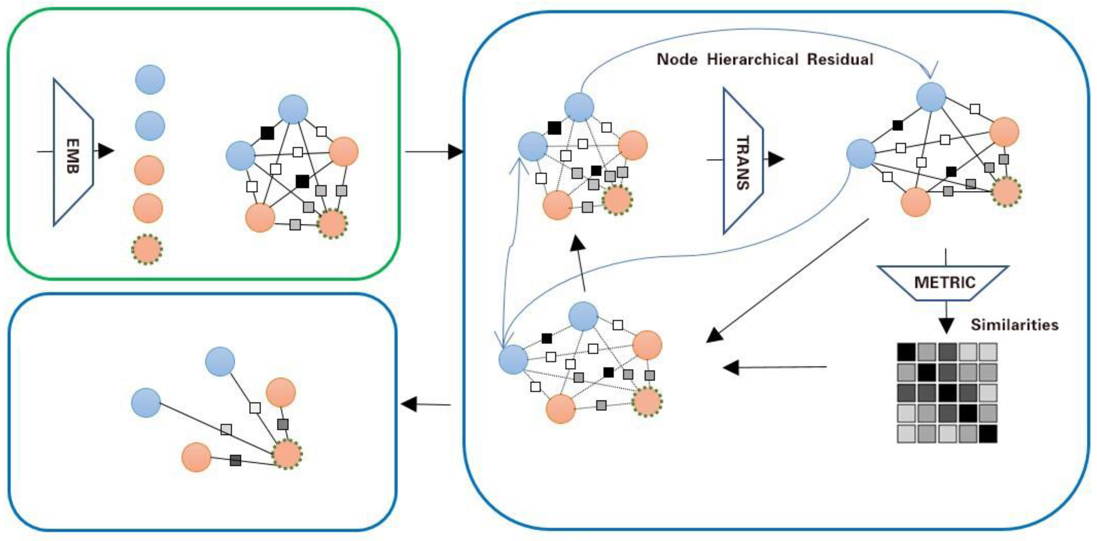
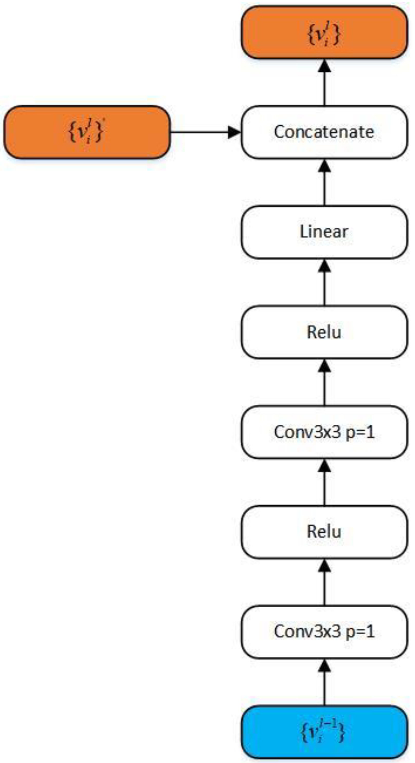
3.2. EGNN + Node Hierarchical Residual Model Architecture

The EGNN + Node Hierarchical Residual for few-shot classification is described in this section. It is seen in Figure 1. An initial fully connected graph is built using the feature representations of all samples for the target task (extracted from a jointly trained Convolutional Neural Network), where each node represents a sample and each edge reflects the sort of link between two connected nodes. Let $G=\left(V;E;T\right)$ represent the graph that was created using samples from the task $T$, with $V:={\left\{V_i\right\}}_{i=1,\dots ,\left|T\right|}$ and $E:={\left\{E_{ij}\right\}}_{i,j=1,\dots ,\left|T\right|}$ standing in for the graph’s node set and edge set, respectively. Let $v_i$ be the node feature and $e_{ij}$ be the edge feature of $V_i$ and $E_{ij}$, respectively. The number of samples in task $T$ as a whole is represented by $\left|T\right|=N\times K+T$. The ground truth node labels describe each ground truth label $y_{ij}$ as follows:

$$y_{ij}=\{\begin{array}{c}1,\hspace{1em}\mathrm{if} y_i=y_j,\hfill \\ 0,\hspace{1em}\mathrm{if} \mathrm{othervise}.\hfill \end{array}$$

(1)

Figure 1. EGNN + Node Hierarchical Residual architecture diagram.

Each edge feature $e_{ij}={\left\{e_{ijd}\right\}}_{d=1}^2\in {[0,1]}^2$ in EGNN + Node Hierarchical Residuals is a two-dimensional vector that depicts the (normalized) strength of the intra-class and inter-class ties that bind two connected nodes. This enables the independent use of cluster-level similarity and cluster-level dissimilarity.

The convolutional embedding network’s output $v_i^0=f_{emb}(x_i;{\theta }_{emb})$, where ${\theta }_{emb}$ stands for the related parameter set, is used to initialize node features (as illustrated in Figure 2a). Edge features are initialized as follows with edge labels:

$$e_{ij}^0=\{\begin{array}{c}[1\Vert 0],\hspace{1em}\mathrm{if} {\mathrm{y}}_{ij}=1 \mathrm{and} i,j\le N\times k,\hfill \\ [1\Vert 0],\hspace{1em}\mathrm{if} {\mathrm{y}}_{ij}=0 \mathrm{and} i,j\le N\times k,\hfill \\ [0.5\Vert 0.5],\hspace{1em}\mathrm{otherwise},\hfill \end{array}$$

(2)

Figure 2. Detailed network architecture used in EGNN + Node Hierarchical Residuals. (a) Embedding network. (b) Feature (node) transformation network. (c) Metric network.

In this case, $||$ signifies the concatenation operation.

EGNNs consist of L layers that process the graph. The forward propagation inference of EGNNs involves the alternating update of node features and edge features.

The node feature in this situation is updated using a neighborhood aggregation procedure given a node $v_i^{l-1}$ and an edge feature $e_{ij}^{l-1}$ in layer $l-1$. A feature transformation is used to update the features of nodes at layer $l$ after aggregating the features of other nodes that are proportional to the edge feature. This produces version $v_i^l$. It works like an attention mechanism by using the edge characteristic $e_{ij}^{l-1}$ from $l-1$ as the contribution from related surrounding nodes:

$$\begin{array}{c}\hfill v_i^l=f_v^l([\sum _j{\tilde{e}}_{ij1}^{l-1}{v}_j^{l-1}\Vert \sum _j{\tilde{e}}_{ij2}^{l-1}{v}_j^{l-1}];{\theta }_v^l)\end{array}$$

(3)

The feature (node) transformation network is represented in the equation by ${\tilde{e}}_{ijd}=\frac{e_{ijd}}{{\displaystyle {\sum }_k{e}_{ijd}}}$, where the parameter set is denoted by ${\theta }_v^l$, as shown in Figure 3b. It is vital to highlight that we take into account inter-cluster aggregation in addition to the traditional intra-cluster aggregation. The target node receives “similar neighbor” information from intra-cluster aggregation while receiving “dissimilar neighbor” information from inter-cluster aggregation. The edge feature update is then carried out using the recently updated node features. In order to update the features of each edge, the (dis)similarity between each pair of nodes is computed, and the prior edge feature values are combined with the updated (dis)similarity as follows:

$$\begin{array}{c}\hfill {\overline{e}}_{ij1}^l=\frac{f_e^l(v_j^l,v_j^l;{\theta }_e^l)e_{ij1}^{l-1}}{{\sum }_k{f}_e^l(v_j^l,v_j^l;{\theta }_e^l)e_{ij1}^{l-1}/\left({\sum }_k{e}_{ik1}^{l-1}\right)}\end{array}$$

(4)

$$\begin{array}{c}\hfill {\overline{e}}_{ij2}^l=\frac{(1-f_e^l(v_i^l,v_j^l;{\theta }_e^l))e_{ij2}^{l-1}}{{\sum }_k(1-f_e^l(v_j^l,v_k^l;{\theta }_e^l))e_{ik2}^{l-1}/\left({\sum }_k{e}_{ik2}^{l-1}\right)}\end{array}$$

(5)

$$e_{ij}^l={\overline{e}}_{ij}^l/|{\overline{e}}_{ij}^l{|}_1$$

(6)

where $f_e^l$ (as illustrated in Figure 2c) is the measurement network that computes similarity scores using the parameter set ${\theta }_e^l$. To be more precise, node features flow into the edges and each member of the edge feature vector is updated from normalized intra-cluster similarity or inter-cluster dissimilarity. In other words, every edge update considers both the relationships between the associated node pairs and the relationships between other pairs of nodes. To determine similarity or dissimilarity, we might decide to employ two different measuring networks. Rather than ($(1-f_{e,sim})$), separate $f_e$; dsims are used.

Figure 3. Convolutional residual structure.

Edge label predictions are obtained from the final edge features, denoted as ${\widehat{y}}_{ij}=e_{ij1}^L$, following updates involving L candidate nodes and edge characteristics. In this instance, ${\widehat{y}}_{ij}\in [0,1]$ can be thought of as the likelihood that nodes $V_i$ and $V_j$ belong to the same class. As a result, based on the support set labels and edge label predictions, each node $V_i$ can be categorized using a straightforward weighted voting method. Node $V_i$’s prediction probability can be expressed as $P(y_i=C_k|T)=p_i^{(k)}$:

$$\begin{array}{c}\hfill p_i^{\left(k\right)}=\mathrm{soft}max\left(\sum _{\{j:j\ne i\wedge (x_i,y_j)\in S\}}{\widehat{y}}_{ij}\delta (y_j=C_k)\right)\end{array}$$

(7)

When $y_j=C_k$ is true, then $\delta (y_j=C_k)$, the Kronecker delta function, is equal to 1; otherwise, it is equal to 0. Graph clustering is a different approach for categorizing nodes. The graph G is first partitioned into clusters using edge predictions and linear programming optimization [24], and each cluster is then labeled with the majority of the support labels it contains. However, to obtain the categorization findings in our study, we merely apply Equation (7). This is the overall algorithm:

Algorithm 1 adds hierarchical residuals between nodes on the basis of the EGNN, and experimental results show that the connection of residuals yields better results than the original approach.

Algorithm 1: EGNN + Node Hierarchical Residual

Input:  $G=\left(V;E;T\right)$ , where $T=S\cup Q$ $S={\{(x_i,y_i)\}}_{i=1}^{N\times K}$ , $Q={\{(x_i,y_i)\}}_{i=N\times K+1}^{N\times K+T}$ Parameters:  ${\theta }_{\mathrm{em}b}\cup {\left\{{\theta }_v^l,{\theta }_e^l\right\}}_{l=1}^L$ Output:  ${\left\{{\widehat{y}}_i\right\}}_{i=N\times K+1}^{N\times K+T}$ Initialize:  $v_i^0=f_{emb}(x_i;{\theta }_{emb})$$, e_{ij}^0$$, \forall i,j$

1: for l = 1,…,L do 2:   /* Node feature update */   3:   for i = 1,…, |V| do 4:    $v_i^l$ ← EdgeUpdate({$v_i^{l-1}$},{$e_{ij}^{l-1}$}, ${\theta }_e^l$ ) 5:  end 6:   /* Edge feature update */ 7:   for (i,j) = 1,…, |E| do 8:    $e_{ij}^l$ ← EdgeUpdate({ $v_i^l$},{$e_{ij}^{l-1}$}; ${\theta }_e^l$) 9:  end 10:    $v_i^l$ ← Hierarchical residual({$v_i^{l-1}$},{$v_i^l$}) 11: end /* Query node label prediction */ 12: ${\left\{{\widehat{y}}_i\right\}}_{i=N\times K+1}^{N\times K+T}$←Edge2NodePred(${\left\{y_i\right\}}_{i=1}^{N\times K}$$,\left\{e_{ij}^L\right\})$

3.3. Training

The suggested EGNN + Node Hierarchical Residual parameters ${\theta }_{emb}\cup {\left\{{\theta }_v^l,{\theta }_e^L\right\}}_{l=1}^L$ are taught end-to-end by minimizing the following loss function given M training tasks, denoted as ${\left\{T_m^{train}\right\}}_{m=1}^M$, training at a certain iteration of the scenario training.

$$\begin{array}{c}\hfill L=\sum _{l=1}^L\sum _{m=1}^M{\lambda }_l{L}_e(Y_{m,e},{\widehat{Y}}_{m,e}^l)\end{array}$$

(8)

For the m-th task in the first layer, $Y_{m,e}$ and ${\widehat{Y}}_{m,e}^l$ represent the sets of all true query edge labels and all (real-valued) query edge predictions, respectively. The binary cross-entropy loss is used to determine the edge loss $L_e$. The total loss includes the losses calculated from all levels to increase gradient flow to lower layers because edge predictions can be acquired not only from the final layer but also from other layers.

4. Experiments

4.1. Datasets

Mini-ImageNet: Mini-ImageNet is one of the most well-liked benchmark datasets for few-shot learning. It was developed by Vinyals et al., contains a subset of ImageNet classes, and was chosen at random from the ImageNet ILSVRC-12 [34] dataset. Each of the 100 classes in mini-ImageNet has 600 image examples. The images are color and 84 × 84 pixels in size. The training set, validation set, and test set are the three segments that make up the mini-ImageNet dataset. There are 64 classes in the training set, 16 classes in the validation set, and 20 classes in the test set [6].

tiered-ImageNet [34]: In contrast to mini-ImageNet, tiered-ImageNet [35] is a subset of the ILSVRC-12 [34] dataset that contains additional categories. A total of 608 categories are included in tiered-ImageNet, and each category has an average of 1281 color photos that are 84 × 84 in size. Tiered-ImageNet, as opposed to mini-ImageNet, uses a tiered classification framework for a wider range of categories, which correlate to higher-level nodes in ImageNet. The 34 top-level categories of tiered-ImageNet are further broken down into 20 training categories (351 total categories), 6 validation categories (97 total categories), and 8 test categories (160 total categories). Since categories frequently form hierarchical structures in real-life situations, where high-level nodes cover numerous low-level nodes, this hierarchical design brings tiered-ImageNet closer to problems involving real-world classification.

Similar to mini-ImageNet, tiered-ImageNet is a benchmark dataset for few-shot learning that can be used to assess and enhance the performance of few-shot learning algorithms. Tiered-ImageNet can more accurately reflect the complexity and variety of real-world classification problems because of its increased number of categories and samples, making it more extensively relevant for studies in few-shot learning and meta-learning [33,36].

The CBAC (Car Brand Appearance Classification): A tiny dataset called CBAC (Car Brand Appearance Classification) was created for this study’s comparison of the performance of few-shot classification. The classification of few-shot images is its main application. The photographs in this collection were obtained from the Autohome website. There are 22 categories in CBAC, and each category features exterior images of various car brands. All of the photographs are in color and have an 84 × 84 pixel dimension. There are 20,254 photos in the CBAC collection. The training set, validation set, and test set are the three segments that make up the CBAC dataset. There are a total of 13,834 photos in the training set, divided among 14 categories, with roughly 1000 images each category. There are roughly 800 photographs each category in both the validation set and test set’s 4 categories, for a total of 3210 images in each set.

4.2. Experimental Setup

Network Architecture: Similar to the majority of few-shot learning models, a Convolutional Neural Network with four blocks is utilized for the feature embedding module. This architecture contains no leftover connections. Each convolutional block is made up of a batch normalization step, a 3 × 3 convolution layer, and a LeakyReLU activation. Figure 2 provides comprehensive descriptions of each network design used in EGNN + Node Hierarchical Residual.

Training: The Adam optimizer is used to train the model on the public datasets, with an initial learning rate of 10⁻³ and a weight decay of 10⁻⁶. The initial learning rate is set to 10⁻⁴ on the CBAC dataset, while the weight decay is set at 10⁻⁶. The batch size for contrastive meta-training tasks is set at 40 in all studies to guarantee a fair comparison with the original EGNN. For mini-ImageNet, the learning rate is reduced by half every 15,000 episodes, while for tiered-ImageNet and CBAC, transfer learning is applied directly from mini-ImageNet, and the learning rate is reduced by half every 20,000 episodes for tiered-ImageNet and every 10,000 episodes for CBAC since it is a larger dataset that requires more iterations to converge.

All code implementations are conducted in PyTorch [37] and executed on an NVIDIA A100 Tensor Core GPU. For the tiered-ImageNet dataset, which is relatively large, it requires physically splitting the dataset into two parts and loading them together, involving at least two NVIDIA A100 GPUs working in parallel.

Residual Structures: In the experiments on the mini-ImageNet dataset, two residual structures are used. The first one is a direct linear connection, and the second one includes a convolutional layer, as illustrated in Figure 3.

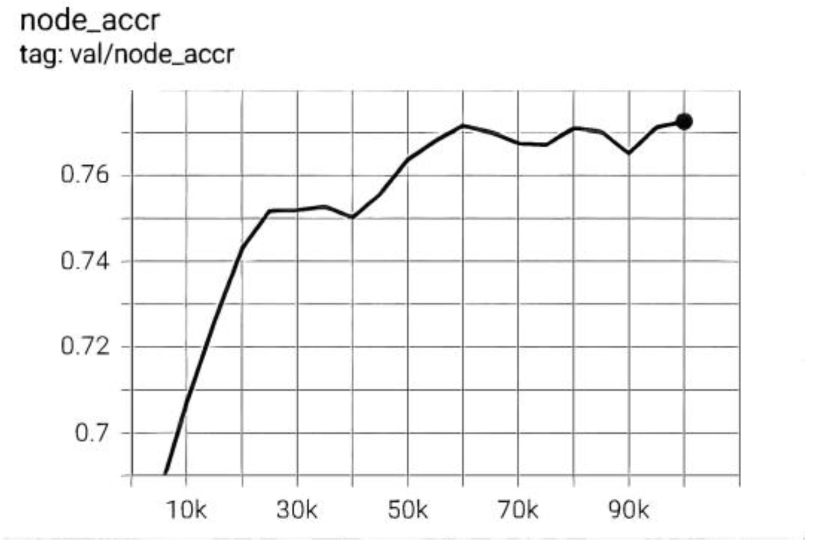
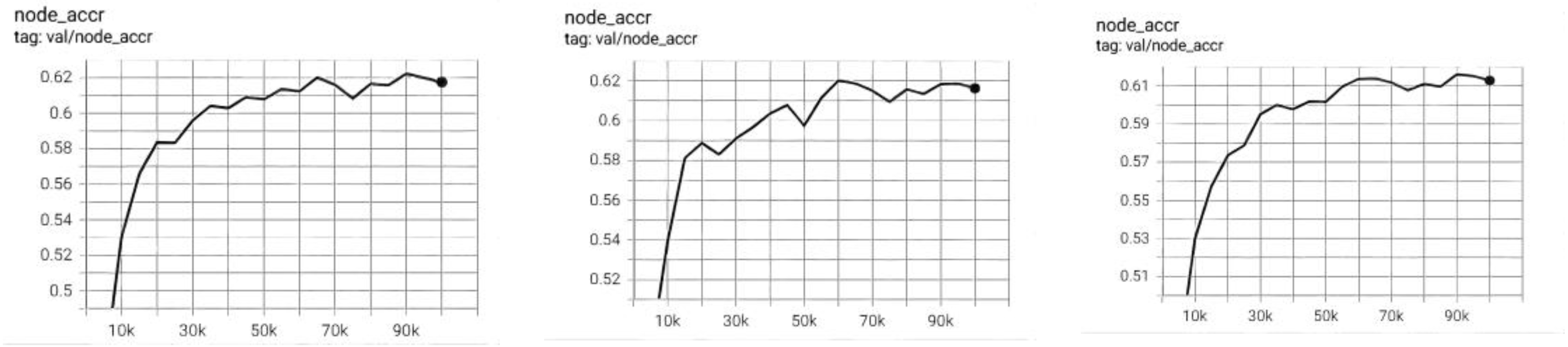
4.3. Results and Analysis

Table 1 and Table 2 present our experimental results on the mini-ImageNet and tiered-ImageNet datasets, respectively. These tables are sorted by method categories. Table 3 displays three comparative experimental results on the CBAC dataset. Note that the results only compare edge-conditioned Graph Neural Networks with prior relevant methods in few-shot image classification. The results in the table are the corresponding accuracies in %. The terms ”5-ways 1-shot” and “5-ways 5-shot” are commonly used in the context of few-shot learning. The term ”5-ways 1-shot” signifies that the model is exposed to only one sample (i.e., one image) from each class within each training set and is subsequently evaluated on its classification capability for these classes in the test set. This implies that the model needs to learn effective feature representations from a limited number of samples to correctly classify new instances. On the other hand, “5-ways 5-shot” indicates that the model is presented with five samples (i.e., five images) from each class within each training set and is then assessed on its classification performance for these classes in the test set. In contrast to “5-ways 1-shot”, “5-ways 5-shot” provides more training samples, enabling the model to acquire richer feature representations.

Table 1. The 1-shot and 5-shot classification results on the mini-ImageNet dataset under the 5-way setting.

	Mode	1-Shot	5-Shot
GNN methods	GNN [17] TPN [38] EGNN [19] EGNN [19] * wDAE-GNN [23] EGNN-NHR EGNN-NHR0	50.30 55.51 58.98 58.34 61.07 ± 0.15 61.68 61.52	66.40 69.86 76.37 76.80 76.75 ± 0.11 77.26 78.55

∗—we implemented using pre-trained feature extractor.

Table 2. The 1-shot and 5-shot classification results on the tiered-ImageNet dataset under the 5-way setting.

	Mode	1-Shot	5-Shot
GNN methods	TPN [38] EGNN [19] EGNN [19] * EGNN-NHR0	59.91 58.98 59.30 60.15	73.30 80.15 80.22 78.11

∗—we implemented using pre-trained feature extractor.

Table 3. The 1-shot and 5-shot classification results on the CBAC dataset under the 5-way setting.

	Mode	1-Shot	5-Shot
GNN methods	GNN [17] EGNN [19] EGNN-NHR0	42.36 49.47 60.61	48.79 57.58 66.88

In experiments, “5-ways 1-shot” and “5-ways 5-shot” tasks are typically employed to evaluate the performance of models, facilitating the comparison of different models in the context of few-shot learning scenarios. These tasks impose significant demands on a model’s generalization and learning capabilities as the model must learn effective feature representations from a limited number of samples and be capable of accurate classification on new instances.

In the table, “EGNN-NHR” refers to the EGNN model with convolutional residual structure (as shown in Figure 3), while “EGNN-NHR₀” refers to the EGNN model with a linear residual structure.

Result Analysis:

In the public dataset mini-ImageNet (as shown in Table 1), both residual connections with convolutional structures and linear residual structures showed significant improvements in experiments. For instance, in the 5-way 1-shot setting on the mini-ImageNet dataset, EGNN-NHR improved by 2.70% over EGNN, while EGNN-NHR₀ improved by 2.54%. In the 5-way 5-shot setting on the mini-ImageNet dataset, EGNN-NHR improved by 0.89% over EGNN, and EGNN-NHR₀ improved by 2.18%. However, an interesting phenomenon was seen: models with convolutional structures showed more improvement in the 5-way 1-shot experiments compared to the 5-way 5-shot experiments. It is possible that if different structures are appropriately designed for each layer, residual connections with convolutional structures might show more improvement with smaller support sets, while linear residual structures could provide more improvement with larger support sets.

In the public dataset tiered-ImageNet (as shown in Table 2), the experiments in the 5-way 1-shot setting showed an increase of 1.17%, while there was a slight decrease in the 5-way 5-shot setting. In tiered-ImageNet experiments, since this dataset is relatively large, it’s possible to fine-tune the knowledge learned from mini-ImageNet directly.

In the public dataset, we observed some intriguing phenomena and results that warrant further in-depth exploration and explanation. A more detailed discussion follows:

Impact of Convolutional and Linear Residual Structures: The experimental results have demonstrated a significant enhancement in model performance upon introducing convolutional and linear residual connections, marking a noteworthy finding. In the context of the 5-way 1-shot task, both EGNN-NHR and EGNN-NHR0 exhibited substantial improvements of 2.70% and 2.54%, respectively. However, in the 5-way 5-shot task, the improvements were comparatively modest, with EGNN-NHR achieving 0.89% and EGNN-NHR0 showing a 2.18% boost. This variance in performance enhancement may be attributed to the varying characteristics of different tasks and datasets. Further research can delve into the underlying reasons why convolutional structures excel in few-shot tasks, while linear residual structures prove more effective in larger-sample scenarios.

Explaining the Performance Dip: A slight decline in performance was observed in the 5-way 5-shot task. This phenomenon might be linked to the complexity of the task and the model’s capacity. More intricate tasks often demand increased learning and representation capabilities, and the relatively larger support sets in 5-shot tasks may contribute to potential overfitting by the model. Additionally, factors such as dataset properties or hyperparameter choices during training could also influence performance.

Future Research Directions: Given the substantial performance gains achieved through the introduction of residual connection structures, future research avenues could explore additional types of residual structures or combinations to further enhance model performance. Diversifying the model by experimenting with different convolutional kernel sizes, channel numbers, or other variants could be considered. Moreover, the application of this residual connection strategy to other tasks and domains warrants investigation to assess its generalizability and applicability.

Improvements in Training and Optimization: Subsequent research efforts could delve into refining the training and optimization processes to mitigate the likelihood of performance degradation. This could involve fine-tuning hyperparameters or employing more sophisticated regularization strategies to address potential overfitting issues. Furthermore, exploring more effective training methods to enhance model robustness is a promising avenue for future exploration.

The image classification accuracy of EGNN-NHR0 on mini-ImageNet-5-way-5-shot can be seen from Figure 4, and the image classification accuracy of EGNN-NHR on mini-ImageNet-5-way-5-shot can be seen from Figure 5 and Figure 6, it can be concluded that as the number of layers increases, the accuracy also increases.

Figure 4. Image classification accuracy of EGNN-NHR₀ on mini-ImageNet-5-way-5-shot.

Figure 5. Image classification accuracy of EGNN-NHR on mini-ImageNet-5-way-5-shot.

Figure 6. Image classification accuracy of EGNN-NHR0 on mini-ImageNet-5-way-1-shot. From left to right: L5, L4, L3, with the highest accuracies being 62.23%, 62.02%, 61.61% respectively.

All of the above points of discussion show improvements in both transductive and non-transductive settings. In particular, EGNN-NHR0 achieved a 1.37% improvement in the mini-ImageNet 5-way 1-shot setting at level L5.

In the self-created CBAC dataset, as shown in Table 3, to demonstrate the significant improvement of the residual structure on EGNN, a dataset was created for classifying the appearances of car brands. This dataset consists of 20,254 color images, categorized into 22 classes. Comparative experiments were conducted on three models, and it was evident that there were notable differences among these models in this small dataset. Specifically, EGNN-NHR0 achieved 60.61% and 66.88% accuracy in the 1-shot and 5-shot settings, respectively, which is a relative improvement of 11.14% and 9.3% compared to the EGNN. To ensure the robustness of this result, comparative experiments were conducted with a GNN model on this dataset.

In explaining possible underlying principles, this could be related to the residual connections in the model architecture and the nature of few-shot learning.

• More improvement with convolutional residual connections in the 5-way 1-shot experiment: This phenomenon might be due to the extremely limited data in the 5-way 1-shot task, where there was only one sample per class for training. Convolutional Residual Connections are better at capturing local features and patterns, making them beneficial for improving model performance in low-data situations. This is because convolutional layers have local receptive fields and are better suited to capturing local patterns, which are more critical in few-shot tasks.
• More significant improvement with linear residual structures with larger support sets: When the support set becomes larger, the model may need to capture global information and relationships more effectively. Linear residual structures are better at propagating global information, hence leading to more significant improvements with larger support sets. In the 5-way 5-shot task, where each class had five samples, having relatively more data allows the model to learn global relationships better.
• Hierarchical design of different structural levels: If you design different levels of residual connections intelligently, you can adapt to support sets of different sizes more effectively. At lower model layers, using convolutional residual connections can help extract local features, while at higher layers, using linear residual connections can capture global relationships better. This hierarchical design leverages the advantages of different structures and enhances performance in various data contexts.

In summary, this subtle phenomenon may be attributed to the need for the model to balance the learning of local features and global relationships in few-shot learning tasks. Different residual connection structures have different advantages in various tasks and data sizes. Therefore, by cleverly designing hierarchical structures, the model can better adapt to different few-shot learning tasks.

5. Conclusions

This study involved the introduction of residual connection structures into the Edge-Conditioned Graph Neural Network (EGNN). This innovative strategy, inspired by the principles of deep residual networks (ResNet), aimed to enhance the model’s information propagation and learning capabilities. Initially designed for few-shot image classification tasks, EGNN had demonstrated remarkable performance in handling limited data.

However, in the mimicked work, the introduction of residual connections between different graph neural layers within EGNN significantly increased the model’s depth and complexity. This adaptation allowed the model to better capture the features and relationships within the data. This mimicking approach bears resemblance to the practice of incorporating residual blocks in ResNet, a widely acknowledged innovation in the field of deep learning.

Consequently, the mimicked work involved the integration of residual connections into EGNN, leading to improved information propagation and learning capabilities. This strategy yielded substantial improvements in accuracy, particularly in the two primary benchmark metrics of 5-way 1-shot and 5-way 5-shot tasks in both public datasets and custom datasets.

As for the scope for improvement, future research can explore further extensions of this concept. Experimenting with different types of residual structures or combinations could potentially enhance the model’s performance. Additionally, investigating the applicability of this residual connection strategy in other tasks and domains would provide insights into its versatility and utility. Further improvements in model training and optimization techniques may also be explored to enhance performance while reducing computational complexity. These directions represent potential avenues for future research, offering the opportunity to advance the fields of graph neural networks and few-shot learning.

6. Innovation and Outlook

In few-shot classification, uncertainty is a critical issue as models need to better estimate the confidence of their predictions. Future research may focus on how to effectively model prediction uncertainty in Graph Neural Networks, thereby providing more reliable decision support. The model architecture of graph neural networks is still evolving, and new structures more suitable for few-shot classification may emerge in the future. These structures may better capture relationships and local patterns in graph data, thus enhancing model performance.

The integration of hierarchical residual techniques in this study injects new vitality and innovation into the field of graph neural networks for few-shot classification. By propagating residual information at each layer, the model can flexibly learn hierarchical features within the data, thereby improving its generalization and classification performance. This approach holds the promise of addressing the challenge of gradient propagation in graph data and facilitating the orderly transmission of information within complex graph structures. Hierarchical residuals also endow Graph Neural Networks with stronger transfer learning and domain adaptation capabilities, opening up greater potential for various practical application scenarios.

In the future, we believe that the innovation of different hierarchical residuals at different layers will lead the development of graph neural networks in the field of few-shot classification, providing more accurate classification results in data-scarce scenarios.

References

1. Deng, J.; Dong, W.; Socher, R.; Li, L.-J.; Li, K.; Li, F. Imagenet: A large-scale hierarchical image database. In Proceedings of the 2009 IEEE Conference on Computer Vision and Pattern Recognition, Miami, FL, USA, 20–25 June 2009; pp. 248–255. [Google Scholar]
2. Simonyan, K.; Zisserman, A. Very deep convolutional networks for large-scale image recognition. arXiv 2014, arXiv:1409.1556. [Google Scholar]
3. Lake, B.; Salakhutdinov, R.; Gross, J.; Tenenbaum, J. One shot learning of simple visual concepts. In Proceedings of the Cognitive Science Society, Boston, MA, USA, 20–23 July 2011; Volume 33. [Google Scholar]
4. Vinyals, O.; Blundell, C.; Lillicrap, T.; Kavukcuoglu, K.; Wierstra, D. Matching networks for one shot learning. In Proceedings of the Advances in Neural Information Processing Systems 29 (NIPS 2016), Barcelona, Spain, 5–10 September 2016; pp. 3630–3638. [Google Scholar]
5. Bertinetto, L.; Henriques, J.F.; Valmadre, J.; Torr, P.; Vedaldi, A. Learning feed-forward one-shot learners. In Proceedings of the Advances in Neural Information Processing Systems 29 (NIPS 2016), Barcelona, Spain, 5–10 September 2016; pp. 523–531. [Google Scholar]
6. Ravi, S.; Larochelle, H. Optimization as a model for fewshot learning. In Proceedings of the International Conference on Learning Representations, Toulon, France, 24–26 April 2017. [Google Scholar]
7. Hariharan, B.; Girshick, R. Low-shot Visual Recognition by Shrinking and Hallucinating Features. In Proceedings of the IEEE International Conference on Computer Vision (ICCV), Venice, Italy, 22–29 October 2017. [Google Scholar]
8. Snell, J.; Swersky, K.; Zemel, R. Prototypical networks for few-shot learning. In Proceedings of the Advances in Neural Information Processing Systems 30 (NIPS 2017), Long Beach, CA, USA, 4–9 December 2017; pp. 4080–4090. [Google Scholar]
9. Raza, H.; Ravanbakhsh, M.; Klein, T.; Nabi, M. Weakly supervised one shot segmentation. In Proceedings of the IEEE International Conference on Computer Vision Workshops, Soeul, Republic of Korea, 27–28 October 2019. [Google Scholar]
10. Xu, Y.; Zhang, Y. Enhancement Economic System Based-Graph Neural Network in Stock Classification. IEEE Access 2023, 11, 17956–17967. [Google Scholar] [CrossRef]
11. Chen, W.-Y.; Liu, Y.-C.; Kira, Z.; Wang, Y.-C.; Huang, J.-B. A closer look at few-shot classification. In Proceedings of the International Conference on Learning Representations, New Orleans, LA, USA, 6–9 May 2019. [Google Scholar]
12. Li, X.; Yang, X.; Ma, Z.; Xue, J. Deep metric learning for few-shot image classification: A review of recent developments. Pattern Recognit. 2023, 138, 109381. [Google Scholar] [CrossRef]
13. Xu, H.; Zhang, Y.; Xu, Y. Promoting Financial Market Development-Financial Stock Classification Using Graph Convolutional Neural Networks. IEEE Access 2023, 11, 49289–49299. [Google Scholar] [CrossRef]
14. Shiyao, X.; Yang, X. Frog-GNN: Multi-perspective aggregation based graph neural network for few-shot text classification. Expert Syst. Appl. 2021, 176, 114795. [Google Scholar]
15. Cen, C.; Kenli, L.; Wei, W.; Zhou, J.T.; Zeng, Z. Hierarchical graph neural networks for few-shot learning. IEEE Trans. Circuits Syst. Video Technol. 2021, 32, 240–252. [Google Scholar]
16. Vaswani, A.; Shazeer, N.; Parmar, N.; Uszkoreit, J.; Jones, L.; Gomez, A.N.; Kaiser, Ł.; Polosukhin, I. At-tention is all you need. In Proceedings of the Advances in Neural Information Processing Systems 30 (NIPS 2017), Long Beach, CA, USA, 4–9 December 2017; pp. 5998–6008. [Google Scholar]
17. Garcia, V.; Bruna, J. Few-shot learning with graph neural networks. arXiv 2017, arXiv:1711.04043. [Google Scholar]
18. Li, H.; Eigen, D.; Dodge, S.; Zeiler, M.; Wang, X. Finding taskrelevant features for few-shot learning by category traversal. In Proceedings of the IEEE Conference on Computer Vision and Pattern Recognition, Long Beach, CA, USA, 16–20 June 2019; pp. 1–10. [Google Scholar]
19. Kim, J.; Kim, T.; Kim, S.; Yoo, C.D. Edge-labeling graph neural network for few-shot learning. In Proceedings of the IEEE Conference on Computer Vision and Pattern Recognition, Long Beach, CA, USA, 16–20 June 2019; pp. 11–20. [Google Scholar]
20. Gori, M.; Monfardini, G.; Scarselli, F. A new model for learning in graph domains. In Proceedings of the 2005 IEEE International Joint Conference on Neural Networks, Montreal, QC, Canada, 31 July–4 August 2005; pp. 729–734. [Google Scholar]
21. Kipf, T.N.; Welling, M. Semi-supervised classification with graph convolutional networks. arXiv 2016, arXiv:1609.02907. [Google Scholar]
22. Zhou, J.; Cui, G.; Zhang, Z.; Yang, C.; Liu, Z.; Wang, L.; Li, C.; Sun, M. Graph neural networks: A review of methods and applications. arXiv 2018, arXiv:1812.08434. [Google Scholar] [CrossRef]
23. Gidaris, S.; Komodakis, N. Generating classification weights with gnn denoising autoencoders for few-shot learning. arXiv 2019, arXiv:1905.01102. [Google Scholar]
24. Kim, S.; Nowozin, S.; Kohli, P.; Yoo, C. Higher-order correlation clustering for image segmentation. In Proceedings of the Advances in Neural Information Processing Systems 24 (NIPS 2011), Granada, Spain, 12–14 December 2011; pp. 1530–1538. [Google Scholar]
25. Gong, L.; Cheng, Q. Adaptive edge features guided graph attention networks. arXiv 2018, arXiv:1809.02709. [Google Scholar]
26. Kipf, T.; Fetaya, E.; Wang, K.-C.; Welling, M.; Zemel, R. Neural relational inference for interacting systems. arXiv 2018, arXiv:1802.04687. [Google Scholar]
27. Johnson, D.D. Learning graphical state transitions. In Proceedings of the 5th International Conference on Learning Representations (ICLR 2017), Toulon, France, 24–26 April 2016. [Google Scholar]
28. Koch, G.; Zemel, R.; Salakhutdinov, R. Siamese neural networks for one-shot image recognition. In Proceedings of the ICML Deep Learning Workshop, Lille, France, 6–11 July 2015; Volume 2. [Google Scholar]
29. Sung, F.; Yang, Y.; Zhang, L.; Xiang, T.; Torr, P.H.; Hospedales, T.M. Learning to compare: Relation network for few-shot learning. In Proceedings of the IEEE Conference on Computer Vision and Pattern Recognition, Salt Lake City, UT, USA, 18–23 June 2018; pp. 1199–1208. [Google Scholar]
30. Cai, Q.; Pan, Y.; Yao, T.; Yan, C.; Mei, T. Memory matching networks for one-shot image recognition. In Proceedings of the IEEE Conference on Computer Vision and Pattern Recognition, Salt Lake City, UT, USA, 18–23 June 2018; pp. 4080–4088. [Google Scholar]
31. Zhang, R.; Che, T.; Ghahramani, Z.; Bengio, Y.; Song, Y. Metagan: An adversarial approach to few-shot learning. In Proceedings of the Advances in Neural Information Processing Systems, Montreal, QC, Canada, 3–8 December 2018; pp. 2365–2374. [Google Scholar]
32. He, K.; Zhang, X.; Ren, S.; Sun, J. Deep Residual Learning for Image Recognition. In Proceedings of the 2016 IEEE Conference on Computer Vision and Pattern Recognition (CVPR), Las Vegas, NV, USA, 27–30 June 2016. [Google Scholar] [CrossRef]
33. Finn, C.; Abbeel, P.; Levine, S. Modelagnostic meta-learning for fast adaptation of deep networks. In Proceedings of the 34th International Conference on Machine Learning (ICML), Sydney, NSW, Australia, 6–11 August 2017. [Google Scholar]
34. Russakovsky, O.; Deng, J.; Su, H.; Krause, J.; Satheesh, S.; Ma, S.; Karpathy, A.; Khosla, A.; Bernstein, M.; Berg, A.C.; et al. Imagenet large scale visual recognition challenge. Int. J. Comput. Vis. 2015, 115, 211–252. [Google Scholar] [CrossRef]
35. Ren, M.; Triantafillou, E.; Ravi, S.; Snell, J.; Swersky, K.; Tenenbaum, J.B.; Zemel, R.S. Meta-learning for semi-supervised fewshot classification. arXiv 2018, arXiv:1803.00676. [Google Scholar]
36. Santoro, A.; Bartunov, S.; Botvinick, M.; Wierstra, D.; Lillicrap, T. Meta-learning with memory-augmented neural networks. In Proceedings of the 33rd International Conference on Machine Learning (ICML), New York, NY, USA, 20–22 June 2016; pp. 1842–1850. [Google Scholar]
37. Paszke, A.; Gross, S.; Chintala, S.; Chanan, G.; Yang, E.; DeVito, Z.; Lin, Z.; Desmaison, A.; Antiga, L.; Lerer, A. Automatic differentiation in pytorch. In Proceedings of the NIPS 2017 Autodiff Workshop, Long Beach, CA, USA, 9 December 2017. [Google Scholar]
38. Liu, Y.; Lee, J.; Park, M.; Kim, S.; Yang, E.; Hwang, S.J.; Yang, Y. Learning to propagate labels: Transductive propagation network for few-shot learning. arXiv 2018, arXiv:1805.10002. [Google Scholar]
Disclaimer/Publisher’s Note: The statements, opinions and data contained in all publications are solely those of the individual author(s) and contributor(s) and not of MDPI and/or the editor(s). MDPI and/or the editor(s) disclaim responsibility for any injury to people or property resulting from any ideas, methods, instructions or products referred to in the content.
Article Metrics
Citations
Article Access Statistics
Multiple requests from the same IP address are counted as one view.