Self-adaptive Artificial Bee Colony with a Candidate Strategy Pool

Abstract

As a newly developed metaheuristic algorithm, the artificial bee colony (ABC) has garnered a lot of interest because of its strong exploration ability and easy implementation. However, its exploitation ability is poor and dramatically deteriorates for high-dimension and/or non-separable functions. To fix this defect, a self-adaptive ABC with a candidate strategy pool (SAABC-CS) is proposed. First, several search strategies with different features are assembled in the strategy pool. The top 10% of the bees make up the elite bee group. Then, we choose an appropriate strategy and implement this strategy for the present population according to the success rate learning information. Finally, we simultaneously implement some improved neighborhood search strategies in the scout bee phase. A total of 22 basic benchmark functions and the CEC2013 set of tests were employed to prove the usefulness of SAABC-CS. The impact of combining the five methods and the self-adaptive mechanism inside the SAABC-CS framework was examined in an experiment with 22 fundamental benchmark problems. In the CEC2013 set of tests, the comparison of SAABC-CS with a number of state-of-the-art algorithms showed that SAABC-CS outperformed these widely-used algorithms. Moreover, despite the increasing dimensions of CEC2013, SAABC-CS was robust and offered a higher solution quality.

1. Introduction

Optimization problems are omnipresent in industrial manufacturing and science activities. In general, these problems are complex and characterized by non-convexity, non-differentiability, discontinuity, etc. These kinds of problem are hard to handle with traditional methods in mathematics because they require strict limits on mathematical properties in optimization problems. In recent years, swarm algorithms (SAs) have received much attention as a powerful tool for solving these kinds of complex optimization problem. Since the need for SAs was recognized, a wide variety of SAs have been developed, often inspired by modeling the behaviors of organisms in the natural world, including the genetic algorithm (GA) [1,2], the firefly algorithm (FA) [3], the ant colony algorithm (ACO) [4], the differential evolution algorithm (DE) [5,6,7], the particle swarm algorithm (PSO) [8,9], and artificial bee colony (ABC) [10,11], etc.

The ABC algorithm, which replicates the tight collaborative activity of employed bees, onlooker bees, and scout bees in discovering suitable food sources, was initially described by Karaboga et al. [12] in 2005. Due to its straightforward design, few variables, and strong resilience, the ABC has attracted researcher interest and is applied in route planning, resource scheduling, and other related problems. However, it is very difficult to apply a single operator to perfectly solve all kinds of optimization problem. The ABC is no exception and faces the following challenges:

• In comparison to other SAs, ABC has a sluggish convergence, due to the 1-D update in the search equation. It is crucial to figure out how to increase the convergence speed to improve ABC’s performance. One difficulty that should be addressed is how to increase the algorithm’s convergence speed, while maintaining high performance, by enhancing the method;
• The problems that can be solved using the artificial bee colony algorithm are limited in variety, due to the simplicity and singularity of the ABC algorithm’s updating method;
• According to certain pertinent literature studies [13], ABC has a significant capacity for exploration because of a single search equation in the evolution process. As a result, a popular area of research is how to improve exploitation, while maintaining exploration.

Many ABC variants have been designed to address these deficiencies, and the modified techniques can be divided into three groups: modifying search equations [14], assembling a multi-strategy [15], and hybridizing other metaheuristic search frameworks [16].

In order to resolve these difficult optimization issues, this study suggests a novel variation of ABC called SAABC-CS, which stands for self-adaptive ABC with a candidate strategy pool. Its main characteristics can be summed up as follows:

• Five alternative search methods are combined to generate a candidate strategy pool that improves ABC’s exploitation capability, without sacrificing exploration capability. In addition, we include multi-dimensional updates in each strategy, which considerably increases the frequency of individual updates and boosts the convergence speed. A self-adaptive method is also suggested for choosing the right search technique. The knowledge from the previous information is used to adaptively update the selection probability of each strategy;
• Our approach, in contrast to other algorithms, performs quite well, without adding additional control parameters when applying each strategy, which is aligned to the artificial bee colony program’s original intention—simplicity and effectiveness;
• By improving the method, we make it more useful for solving actual, practical issues in the real world.

The remaining part of this paper is divided into the following sections: The works pertaining to the fundamental ABC and its variations are detailed in Section 2. In Section 3, the suggested algorithm SAABC-CS is described. The effectiveness of our suggested approach and the analysis of the results of our algorithm in comparison to other algorithms are provided in Section 4. The last Section provides a summary of our work.

2. Related Work

2.1. ABC Algorithm

The initialization period, employed bee period, onlooker bee period, and scout bee period make up the primary foundation of the ABC. All bees have different responsibilities at different stages. It should be noted that each bee has its own food resources in each period, and the number of bees in each period is consistent. The food resource in this statement often represents a candidate solution to the optimization problem. The evolution framework of the ABC is seen in Figure 1.

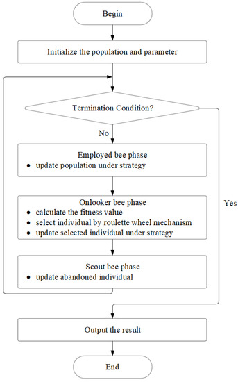
Figure 1. The ABC framework.

Like all SAs, the ABC needs to go through an initialization stage before performing the other three stages of work cyclically. The following are the relevant contents of each phase:

(i)

Initialization phase

In this phase, the entire population is randomly initialized, each individual represents a food resource and this is generated using Equation (1).

$$X_{i,j}=Lower+rand·(Upper-Lower)$$

(1)

where $i=1,2,\cdots ,SN$ and $j=1,2,\cdots ,D$. D stands for the dimension of the optimization problems, while $SN$ is the number of solutions in a swarm. $rand$ is a random number belonging to (0,1), $X_{i,j}$ represents the element of jth dimension of the ith individual. $Lower$ and $Upper$ denote the minimum value and maximum value in all dimensions of each individual, respectively.

(ii)

Employed bee phase

The evolution reaches the employed bee phase after startup. According to Equation (2), each employed bee searches the full search area for new food sources during this phase.

$$V_{i,j}=X_{i,j}+{\varphi }_{i,j}·(X_{i,j}-X_{k,j})$$

(2)

The random number ${\varphi }_{i,j}$ has the value (−1,1). Unlike $X_i$, which belongs to the whole population, $X_k$ is a randomly chosen solution. The value of $V_{i,j}$ is reinitialized using Equation (1) if it oversteps either the lower or higher barrier. $V_i$ takes the place of $X_i$ if its object function value is superior to that of $X_i$.

In addition, there are a number of updated individuals (NUI) for each solution. Thus, NUI is recorded using a 1·SN matrix. At the beginning, every element of NUI is initialized to zero. After that, once the $X_i$ has successfully been replaced by $V_i$, the ith value of NUI is reset to zero. Otherwise, the ith value of NUI is increased by one. The NUI matrix has an effect on the subsequent scout bee phase.

(iii)

Onlooker bee phase

The bee continues to search for new food sources during the onlooker bee phase. In contrast to the employed bee phase, the onlooker bee only has to seek in the vicinity of the chosen food resource, which is equivalent to expanding the utilization of the food resource. At this stage, not every food resource can be selected to search in its vicinity, but a probability search is carried out according to its fitness value. The calculation equation for the fitness value is as shown in Equation (3).

$$Fi{t}_i=\left\{\begin{array}{cc}{\displaystyle \frac{1}{1+f\left(X_i\right)}}\hfill & \mathrm{if}f\left(X_i\right)\ge 0\hfill \\ 1+abs\left(f\left(X_i\right)\right)\hfill & \mathrm{otherwise}\hfill \end{array}\right.$$

(3)

where $Fi{t}_i$ and $f\left(X_i\right)$ are the fitness values of $X_i$ and objective function result, correspondingly. $f\left(X_i\right)$ is calculated in the employed bee phase. Equation (4) determines the selection probability of each food resource.

$$p_i={\displaystyle \frac{Fi{t}_i}{{\sum }_{j=1}^{SN}Fi{t}_j}}$$

(4)

After that, the onlooker bees use the classic roulette wheel selection strategy to select a food resource. Obviously, the larger the fitness value obtained, the greater the chance the food resource is selected. Equation (2) is also used as an update equation for the onlooker bees. In addition, the same process is used as for the employed bees after generating a candidate solution.

(iv)

Scout bee phase

At scout bee phase, the element value NUI associated with each individual is checked. Once an individual’s NUI exceeds a predefined value, it is believed that this food resource has been exhausted, which implies that the individual may be trapped at a local optima. As a result, in this circumstance, the employed bee is transformed into a scout bee to help Equation (1) generate new solutions.

2.2. ABC Variants

Although the ABC algorithm has a good optimization performance, it also has certain shortcomings, such as it being easy to fall into local optimum, the imbalance between exploration and exploitation, and a slow convergence speed. Due to the existing problems with the ABC, researchers have proposed many different methods to solve them. Most solutions can be divided into three distinct categories:

(1)

Modifying the search equation

The performance of the ABC algorithm depends heavily on the solution search equation. In a basic ABC, the solution search equation does well in exploration but poorly in exploitation, since each individual $X_k$ shown in Equation (2) is chosen randomly from the overall population. Thus, inspired by [17,18], Wang and Zhou et al. [19] proposed an ABC variant (KFABC). KFABC is based on knowledge fusion and its viability was tested against 32 benchmark functions. Lu et al. [20] designed Fast ABC (FABC), which made use of two extra alternative search equations for employed bees and onlooker bees, respectively. These two equations also utilized the bees’ individual information and employed a Cauchy operator to equilibrize the global and local search capacities of individuals. In order to prove its effectiveness, the performance of FABC was compared with that of 10 benchmark functions and a genuine path planning issue. Gao et al. [21], inspired by differential evolution (DE), presented an improved search equation using a modified ABC (MABC). This variant enabled the bees to search around the best solutions found in the previous iteration, to improve the exploitation. A total of 28 benchmark functions were used in the comparison experiments. When compared to two ABC-based algorithms, the findings showed that MABC performed well when addressing complicated numerical optimization problems.The improved algorithm that Guo et al. [22] developed based on MABC is called the global artificial bee colony search algorithm. Guo incorporated all the employed bees’ historical best positions based on the information about food sources into the search equations to develop this algorithm. Yu et al. [23] proposed another form of ABC variant called the adaptive ABC (AABC). It adjusted the greedy degree of the original ABC using a novel greedy position update strategy and an adaptive control scheme. Using a set of benchmark functions, AABC outperformed the original ABC and subsequent ABC iterations in their tests.

(2)

Hybridizing another metaheuristic search framework

Hybrid algorithms are mainly based on the combination of two or more metaheuristic algorithms, so that the advantages of one algorithm can be used to offset the deficiencies of other algorithms. This method could improve the optimization performance of an algorithm. The following are some examples of hybrid ABC algorithms that combined the ABC algorithm with other heuristic algorithms. Jadon et al. [24] proposed a hybridization of ABC and DE algorithms (HABCDE), to develop a more efficient algorithm than ABC or DE individually. Over twenty test problems and four actual optimization issues were used to evaluate the performance of HABCDE. Alqattan et al. [25] presented a hybrid particle movement ABC algorithm (HPABC). This algorithm adapted the particle moving process to improve the exploitation of the original ABC variant. The algorithm variant was provided, and seven benchmark functions were utilized to validate it. Chen et al. [26], on the other hand, introduced a simulated annealing algorithm into the employed bees’ phase and proposed the simulated annealing-based ABC algorithm (SAABC). To improve algorithm exploitation, the simulated annealing algorithm was added in the employed bee search process. The experimental results were validated against a collection of numerical benchmark functions of varying size. This demonstrated that the SAABC algorithm outperformed the ABC and global best guided ABC algorithms in the majority of tests.

(3)

Assembling multi-strategy

Multi-strategy search refers to the implementation of different search strategies in the different search stages of the ABC or for different food resources. In recent years, some algorithms that introduced multi-strategy search into ABC have been proposed, but their effectiveness varied. Gao et al. [27] formed a strategy pool using three distinct search strategies and adopted an adaptive selection mechanism to further enhance the performance of the algorithm. It was evaluated using a set of 22 benchmark functions and compared against other ABCs. In almost every case, the comparison findings revealed that the suggested method provided superior results. Song et al. [28] designed a novel algorithm called MFABC. MFABC improved the search ability of the ABC algorithm with a small population by fusing multiple search strategies for both employed bees and onlooker bees. MFABC’s accuracy, stability, efficiency, and convergence rate were demonstrated experimentally on a set of benchmark functions. Chen et al. [29] proposed a new algorithm called self-adaptive differential artificial bee colony (sdABC) by incorporating multiple diverse search strategies and a self-adaptive mechanism into the original ABC algorithm. The sdABC technique was tested on 28 benchmark functions, including both common separable and difficult non-separable CEC2015 functions. The experimental findings suggested that sdABC obtained substantially better outcomes on both separable and non-separable functions than earlier ABC algorithms. In addition to the above ABC algorithm variants, Zhou et al. [30] developed a modified neighborhood search operator by utilizing an elite group, which is called MGABC. Their experiments employed 50 well-known test functions and one real-world optimization issue to validate the technique, which included 22 scalable basic test functions and 28 complicated CEC2013 test functions. The comparison included seven distinct and well-established ABC variations, and the findings suggested that the technique could obtain test results that were at least equivalent in test performance for most of the test functions.

Assessing these three improvement directions, the first is too simple and the second makes the algorithm extremely complicated. Thus, we choose the third direction as our main interest. We based our research partially on prior work from other researchers. By assembling a multi-strategy search, a wider range of issues can be tackled and the outcomes are better.

3. The Proposed Algorithm SAABC-CS

3.1. Candidate Strategy Pool

In most cases, different problems have different characteristics, and they are hard to describe clearly in advance. Thus, problems are usually black boxes. Moreover, different update strategies for ABC have unique characteristics. It is unrealistic to rely on only one strategy to solve all problems. These observations make us reconsider how to select strategies or construct novel strategies to improve the robustness when facing different problems. Based on the motivations above, we selected five search strategies with different characteristics from the relevant literature [18,31] to construct our candidate strategy pool. In addition, we employed the binomial crossover method to enable the algorithm to find optimal solutions more effectively. Considering both exploration and exploitation during the entire evolution process, five strategies were selected and are described in detail, as follows:

(i)

“rand”:

$$\begin{array}{cc}& V_{i,j}=X_{r1,j}+{\varphi }_{i,j}·(X_{r1,j}-X_{r2,j})\end{array}$$

(5)

(ii)

“pbest-1”:

$$\begin{array}{cc}& V_{i,j}=X_{e,j}+{\varphi }_{i,j}·(X_{r1,j}-X_{r2,j})\end{array}$$

(6)

(iii)

“pbest-2”:

$$\begin{array}{cc}& V_{i,j}=X_{e,j}+{\varphi }_{i,j}·(X_{r1,j}-X_{r2,j})+{\phi }_{i,j}·(X_{r3,j}-X_{r4,j})\end{array}$$

(7)

(iv)

“current-to-pbest”:

$$\begin{array}{cc}& V_{i,j}=X_{i,j}+{\varphi }_{i,j}·(X_{i,j}-X_{r1,j})+{\phi }_{i,j}·(X_{e,j}-X_{i,j})\end{array}$$

(8)

(v)

“pbest-to-rand”:

$$\begin{array}{cc}& V_{i,j}=X_{e,j}+{\varphi }_{i,j}·(X_{e,j}-X_{i,j})\end{array}$$

(9)

where $X_{r1}$, $X_{r2}$, $X_{r3}$, and $X_{r4}$ are the different individuals selected randomly in the population, and they are all distinctive from $X_i$. A homogeneous random number between [−1,1] is ${\varphi }_{i,j}$. A solution from an elite group is represented by $X_e$. The top q·SN solutions are chosen to form the elite group, after all the individuals are sorted according to their fitness values. The size of the elite group is controlled by q, which is set at 0.1. ${\phi }_{i,j}$ is a homogeneous random number between [0,1.5].

Figure 2 roughly depicts the behavior of each strategy, the individuals in ellipse are the elite individuals, and the remaining triangle icons represent other common individuals. The red circle in Figure 2 represents the new individual generated by the corresponding strategy. With the “rand” strategy, the position of the new individual in Figure 2a is between two different individuals, and it is close to the first random individual. Actually, its position falls within a circle with $X_{r1}$ as the center and $|X_{r1}-X_{r2}|$ as the radius. The behavior of the “rand” strategy makes the algorithm focus more attention on a global search. Similarly, the position of the new individual in Figure 2b is between an elite individual and two different common individuals with the “pbest-1” strategy. This strategy leads the algorithm to learn the elite’s information, while focusing on a global search. With the “pbest-2” strategy, the position of the new individual in Figure 2c is also in the center of the selected individuals, this makes our algorithm utilize more individual sampling information. As shown in Figure 2d, the position of the new individual is affected by the current individual, an elite individual, and a randomly selected individual in the “current-to-pbest" strategy. The position of the new individual in Figure 2e is based on the elite individual and current individual, which comprehensively takes the current individual and elite individual into consideration.

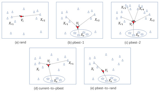
Figure 2. Schematic diagrams of five different strategies. (Stars represent elite individuals, triangles represent common individuals, red circles represent new individual, dashed arrows represent search direction).

In order to further reflect the different characteristics of the five strategies in seeking optimal solutions, we performed an experiment on the Rastrgin function [32] under the same conditions. The formula of Rastrigin is as follows, and its dimension was set to 2:

$$f\left(X\right)=10·D+{\displaystyle \sum _{i=1}^D}[X_i^2-10·\cos (2·\pi ·X_i)]$$

(10)

where X is a 2-dimensional individual.

In this experiment, we obtained the two-dimensional individual distribution for the five strategies after 20 generations, and present the results in Figure 3. The initial population size of each strategy was 100. From Figure 3a, these individuals may be seen to disperse around local maxima, although the local maxima are still distant from the global maxima. Thus, it is obvious that the “ABC/rand” strategy has a strong exploration ability but weak exploitation ability. We can see clearly that all individuals converge around one local optimum in Figure 3b, but the local optimum is not the global optimum. Thus, it has a strong exploitation ability but weak exploration ability. The “ABC/pbest-2” strategy originates from “ABC/pbest-1”, but with increased exploration ability. This modification causes most individuals to distribute around global optimum, with some individuals located around other local optima. The results in Figure 3c further demonstrate that the “ABC/pbest-2” strategy increased its exploration ability while keeping its exploitation ability. As for the results in Figure 3d, the “ABC/current-to-pbest” strategy uses the information of the current individual, a random different individual, and a random elite individual. Thus, it has a strong exploration ability during early generation and a strong exploitation ability during late generation. As we can see from Figure 3e, under the influence of “ABC/pbest-to-rand”, the individuals mainly converged around the global optimum, with others also located near local optima. This was dominated by $X_e$ but also uses the current individual information. Thus, it maintains a significant capacity for exploitation, while also having the opportunity to leave the local optima and go to a global or nearby one.

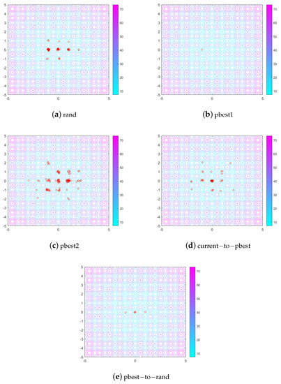
Figure 3. Five strategies’ contour graphs based on the two-dimensional Rastrigin function. (Red dots represent individuals. Subfigures (a–e) represent individual distribution map of the five strategies in the current generation, respectively).

With the exception of the “ABC/rand” technique, the other four search methods all utilize the information of the elite group. The following two benefits result from using an elite group instead of the elite with the best fitness:

(1) In the first place, this allows the entire population to fully utilize the knowledge of the elite solution group during the evolution process and evolve in a better way.

(2) Second, the whole population is prone to becoming locked in local optima if the population only uses the present global optimal solution as the search traction. However, the population may evolve in numerous good directions and are provided better solutions by the elite group. As a result of using an elite group, it is simple for the population to move away from the local optima and reach the global or approximated optimal region.

Additionally, the original ABC search approach performs poorly for some issues with variable inseparability, since it only updates one variable at a time. Therefore, to update many dimensions at once, these techniques combine mutation and crossover, as in GA. In this approach, using various update techniques inside the adaptive mechanism enhances the algorithm’s efficiency, while simultaneously strengthening its robustness. Thus, to create a trial vector $U_{i,j}$, we apply a binomial crossover operator to $X_{i,j}$ and $V_{i,j}$.

$$U_{i,j}=\left\{\begin{array}{cc}{V}_{i,j}\hfill & \mathrm{if}\mathrm{rand}\le \mathrm{M}\mathrm{or}\mathrm{j}=\mathrm{k}\hfill \\ X_{i,j}\hfill & \mathrm{Otherwise}\hfill \end{array}\right.$$

(11)

where $i=1,2,\dots ,SN$, $j=1,2,\dots ,D$. A number chosen at random between [1, D] called k is utilized to make certain that at least one element is updated. $rand$ is an arbitrary number ranging from 0 to 1 with a uniform distribution.

In our algorithm, we also precisely apply the boundary correction technique to improve the outcome. If the jth dimension element of $U_i$ is outside of the boundary, we make the following revisions:

$$U_{i,j}=\left\{\begin{array}{cc}Lower\hfill & \mathrm{if}{U}_{i,j}<\mathrm{Lower}\hfill \\ Upper\hfill & \mathrm{if}{U}_{i,j}>\mathrm{Upper}\hfill \end{array}\right.$$

(12)

To join the following generation, we choose the superior source vector $X_i$ over the trial vector $U_i$.

$$X_i^{G+1}=\left\{\begin{array}{cc}{U}_i\hfill & \mathrm{if}f\left(U_i\right)<f\left(X_i\right)\hfill \\ X_i\hfill & \mathrm{otherwise}\hfill \end{array}\right.$$

(13)

The following values are set for the strategy’s self-definition parameters: The elite community’s size is q·SN. The dimension update is controlled by parameter M, which is set at 0.5.

3.2. Self-adaptive Mechanism

To maximize the algorithm’s efficiency, we must choose a more appropriate approach in different phases of the algorithm, due to the distinctive characteristics of the aforementioned five alternative search strategies. As a result, we include an adaptive mechanism in our suggested algorithm, to choose the best strategy. The fundamental principle of self-adaptation is to dynamically modify the potential for choosing an appropriate approach, in accordance with the success information about producing superior solutions. The selection likelihood of one strategy increases when an exceptional solution is produced by this strategy. Additionally, any tactic has the chance to be picked out during the evolution, owing to the roulette selection system. Such a self-adaptive system can help the population move beyond the local ideal, as well as toward the optimal. The combination of this self-adaptive mechanism with the aforementioned five techniques is depicted in the flowchart in Figure 4.

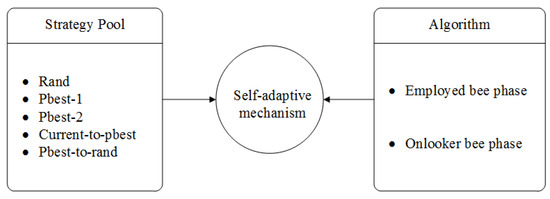
Figure 4. Flowchart of self-adaptive multiple strategies.

In the initialization phase, some variables are initialized by the self-adaptive mechanism. Prob is a 1 × 5 matrix, in which each element $Pro{b}_i$ corresponds to the selection probability for the above $strateg{y}_i$, and the sum of all elements is 1. In the beginning, their selection probability is equal, to guarantee fairness. Two 1 × SN matrices sFlag and fFlag are used, to mark whether the candidate solution is better or worse than the original solution when using a corresponding strategy. SN is a measure of population density. If the new generated solution is better, the associated sFlag matrix element is set to 1 and the corresponding fFlag matrix element is set to 0, and vice versa. We also use two 5·LP matrices, sCounter and fCounter, to count the proportion of triumphs and failures of each generation in the LP generation, after updating using the corresponding strategy. LP represents a fixed interval, and we set this to 10 here. For every LP generation, we use sCounter and fCounter to update the Prob of each strategy. The statistical data information of sCounter and fCounter are the main source for updating the Prob value. Moreover, every time the selected strategy probability is updated, every element of sFlag, fFlag, sCounter, and fCounter must be reset to 0, to avoid affecting the next LP generations. The update equation of Prob is determined using the following Equation (14), and then the probability is normalized using Equation (15).

$$Pro{b}_i=\left\{\begin{array}{c}{\displaystyle \frac{{\sum }_{k=1}^{LP}sCounter\left[i\right]\left[k\right]}{{\sum }_{k=1}^{LP}sCounter\left[i\right]\left[k\right]+{\sum }_{k=1}^{LP}fCounter\left[i\right]\left[k\right]}}\hfill \\ \\ {\sum }_{k=1}^{\mathrm{LP}}\mathrm{sCounter}\left[i\right]\left[k\right]\ne 0\hfill \\ \\ 0.5·Pro{b}_i\mathrm{Otherwise}\hfill \end{array}\right.$$

(14)

$$Pro{b}_i={\displaystyle \frac{Pro{b}_i}{{\sum }_{i=1}^{5}Prob\left(i\right)}}$$

(15)

3.3. Scout Bee and Modified Neighborhood Search Operator

In this stage, we utilize the method proposed by Wang et al. in KFABC [19], adding two methods based on opposition-based learning(OBL) and the Cauchy approach, to generate two additional solutions. Then, we select the best solution from the random solutions, OBL solution, and Cauchy solution, to replace the abandoned solution. The random operator, the OBL operator, and Cauchy disturbance operator that produce the candidate solutions are described in Equations (1), (16) and (17).

$$O{X}_j=Lower+Upper-X_{a,j}$$

(16)

where the space’s boundary is defined by Lower and Upper. j = 1, 2,…, D, and the abandoned solution is represented by $X_a$.

$$C{X}_j=X_{a,j}+Cauchy\left(\right)$$

(17)

where $j=1,2,\dots ,D$, $Cauchy\left(\right)$ return a value from the Cauchy distribution.

In addition, we use a neighborhood search operator in our method as a supplementary operator, which was suggested by Zhou et al. in MGABC [30]. The operator continues to use the data from the elite group solution and determines whether to employ the supplemental operator in this generation based on a certain possibility p (p is 0.1, as in MGABC [30]. The operator is shown in Equation (18).

$$T{X}_i=r1·X_i+r2·X_{e1}+r3·(X_{e2}-X_{e3})$$

(18)

where three solutions from the elite group, $X_{e1}$, $X_{e2}$, and $X_{e3}$, were chosen at random and must be distinct from $X_i$. As positive numbers drawn at random from (0,1), r1, r2, and r3 must also satisfy the restriction that r1 + r2 + r3 = 1. If $T{X}_i$ is superior to $X_i$, $T{X}_i$ will take the place of $X_i$.

3.4. Framework of SAABC-CS

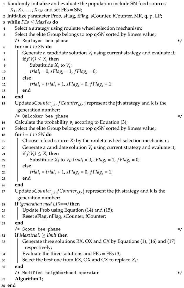
During the employed and onlooker bee phase, SAABC-CS employs five distinct search algorithms, four of which make use of knowledge from the elite group. We provide an adaptive mechanism based on prior knowledge to choose the best search technique, in order to make better use of these five tactics. To enhance the algorithm’s efficiency and speed of convergence, we update the search technique used for the scout bee and add an additional neighborhood search operator. The pseudo-code for SAABC-CS is provided in Algorithms 1 and 2 and, the flowchart for it can be viewed in Figure 5, which help to better explain the entire process.

Algorithm 1: The pseudo-code of Modified neighborhood operator

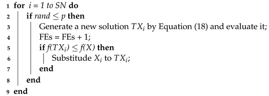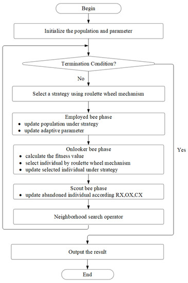
Figure 5. Flowchart of SAABC-CS.

Algorithm 2: The pseudo-code of SAABC-CS.

4. Experiments

4.1. Test Problems

We ran trials on 50 test issues that were separated into two sets of benchmarks, to demonstrate the efficacy of our suggested algorithm SAABC-CS. The first benchmark set included 22 basic functions, and the second benchmark set was referred to as CEC2013. The dimensions of the CEC2013 benchmarks were set as 30, 50, and 100. We used two values (Mean and Std) as metrics for algorithm comparison. ”Mean” represents the average value of the optimal results obtained by the algorithm for the corresponding running times, and “Std” represents the corresponding variance. Experiment 1 not only verified the effectiveness of the strategy pool but also demonstrated the effectiveness of the self-adaptive method. Experiment 2 compared the performance of SAABC-CS with that of the other five algorithms in the CEC2013 function set. All algorithms designed in this section were utilized in MATLAB R2020a. Table 1, Table 2, Table 3 and Table 4 report the compared results, in which the best result for each problem is marked in bold, and summarize the statistical findings. “+/=/−” indicate that SAABC-CS outperformed, was comparable to, or underperformed the compared algorithm in the test tasks.

Table 1. Results of five single strategies vs. multi-strategy ABC algorithms with self-adaptive/rand on basic 22 function (D = 30).

Function		ABC-Rand	ABC-Pbest-1	ABC-Pbest-2	ABC-Current-to-Pbest	ABC-Pbest-to-Rand	RABC-CS	SAABC-CS
F1	Mean	$2.248526\times {10}^{-120}$ +	$7.064515\times {10}^{-113}$ +	$6.559319\times {10}^{-98}$ +	$8.878308\times {10}^{-117}$ +	$8.129275\times {10}^{-176}$ +	$4.189678\times {10}^{-128}$ +	$\mathbf{2}.\mathbf{259275}\times {\mathbf{10}}^{-\mathbf{176}}$
	Std	$1.131182\times {10}^{-119}$	$1.988608\times {10}^{-112}$	$1.662559\times {10}^{-97}$	$4.071247\times {10}^{-116}$	$0.000000\times {10}^0$	$9.079933\times {10}^{-128}$	$0.000000\times {10}^0$
F2	Mean	$4.119521\times {10}^{-62}$ +	$3.388025\times {10}^{-90}$ +	$3.362581\times {10}^{-49}$ +	$4.777346\times {10}^{-59}$ +	$1.004464\times {10}^{-56}$ +	$4.135273\times {10}^{-65}$ +	$8.188025\times {10}^{-91}$
	Std	$8.821390\times {10}^{-62}$	$6.589025\times {10}^{-90}$	$6.925141\times {10}^{-49}$	$8.332598\times {10}^{-59}$	$2.159204\times {10}^{-56}$	$6.097771\times {10}^{-65}$	$7.509025\times {10}^{-90}$
F3	Mean	$7.906320\times {10}^{-95}$ +	$9.642783\times {10}^{-89}$ +	$8.755489\times {10}^{-83}$ +	$3.004974\times {10}^{-94}$ +	$5.845769\times {10}^{-125}$ +	$3.300380\times {10}^{-100}$ +	$6.201979\times {10}^{-130}$
	Std	$2.782121\times {10}^{-94}$	$5.162428\times {10}^{-88}$	$2.132246\times {10}^{-82}$	$1.363288\times {10}^{-93}$	$2.367933\times {10}^{-124}$	$1.234790\times {10}^{-99}$	$2.101411\times {10}^{-129}$
F4	Mean	$5.442075\times {10}^{-54}$ +	$1.176991\times {10}^{-50}$ +	$1.281191\times {10}^{-45}$+	$7.984461\times {10}^{-52}$ +	$5.442075\times {10}^{-54}$ +	$2.471204\times {10}^{-56}$+	$2.899439\times {10}^{-80}$
	Std	$6.026015\times {10}^{-54}$	$1.601701\times {10}^{-50}$	$2.159118\times {10}^{-45}$	$1.749531\times {10}^{-51}$	$6.026015\times {10}^{-54}$	$6.575316\times {10}^{-56}$	$1.518933\times {10}^{-80}$
F5	Mean	$2.466807\times {10}^1$ +	$2.575768\times {10}^1$ +	$2.523777\times {10}^1$ +	$2.543241\times {10}^0$ +	$2.076386\times {10}^1$ +	$2.402630\times {10}^1$ +	$2.352532\times {10}^0$
	Std	$8.280997\times {10}^{-2}$	$1.369552\times {10}^{-1}$	$1.217680\times {10}^{-1}$	$1.025347\times {10}^{-1}$	$1.479236\times {10}^{-1}$	$1.590104\times {10}^{-1}$	$2.352992\times {10}^0$
F6	Mean	$\mathbf{0}.\mathbf{000000}\times {\mathbf{10}}^{\mathbf{0}}$ =	$\mathbf{0}.\mathbf{000000}\times {\mathbf{10}}^{\mathbf{0}}$ =	$\mathbf{0}.\mathbf{000000}\times {\mathbf{10}}^{\mathbf{0}}$ =	$\mathbf{0}.\mathbf{000000}\times {\mathbf{10}}^{\mathbf{0}}$ =	$\mathbf{0}.\mathbf{000000}\times {\mathbf{10}}^{\mathbf{0}}$ =	$\mathbf{0}.\mathbf{000000}\times {\mathbf{10}}^{\mathbf{0}}$ =	$\mathbf{0}.\mathbf{000000}\times {\mathbf{10}}^{\mathbf{0}}$
	Std	$0.000000\times {10}^0$	$0.000000\times {10}^0$	$0.000000\times {10}^0$	$0.000000\times {10}^0$	$0.000000\times {10}^0$	$0.000000\times {10}^0$	$0.000000\times {10}^0$
F7	Mean	$9.141111\times {10}^{-4}$ +	$1.382338\times {10}^{-3}$ +	$1.491601\times {10}^{-3}$ +	$\mathbf{1}.\mathbf{119361}\times {\mathbf{10}}^{-\mathbf{4}}$ =	$5.043735\times {10}^{-4}$ +	$1.060796\times {10}^{-3}$ +	$\mathbf{1}.\mathbf{119325}\times {\mathbf{10}}^{-\mathbf{4}}$
	Std	$3.535380\times {10}^{-4}$	$5.575281\times {10}^{-4}$	$6.834976\times {10}^{-4}$	$5.475349\times {10}^{-4}$	$2.076206\times {10}^{-4}$	$4.821712\times {10}^{-4}$	$7.547842\times {10}^{-4}$
F8	Mean	$2.936318\times {10}^{-116}$ +	$1.231300\times {10}^{-109}$ +	$4.147755\times {10}^{-173}$ +	$3.719664\times {10}^{-114}$ +	$1.126064\times {10}^{-93}$ +	$8.024818\times {10}^{-125}$ +	$\mathbf{4}.\mathbf{575380}\times {\mathbf{10}}^{-\mathbf{181}}$
	Std	$1.574936\times {10}^{-115}$	$3.518575\times {10}^{-109}$	$0.000000\times {10}^0$	$9.643898\times {10}^{-114}$	$4.557991\times {10}^{-93}$	$1.676287\times {10}^{-124}$	$2.053852\times {10}^{-180}$
F9	Mean	$1.600553\times {10}^{-177}$ +	$1.534562\times {10}^{-113}$ +	$3.379257\times {10}^{-99}$ +	$1.924197\times {10}^{-117}$ +	$2.223761\times {10}^{-122}$ +	$5.549013\times {10}^{-128}$ +	$\mathbf{4}.\mathbf{336995}\times {\mathbf{10}}^{-\mathbf{185}}$
	Std	$0.000000\times {10}^0$	$5.281619\times {10}^{-113}$	$1.046764\times {10}^{-98}$	$7.117055\times {10}^{-117}$	$6.496603\times {10}^{-122}$	$2.377221\times {10}^{-127}$	$1.740039\times {10}^{-185}$
F10	Mean	$\mathbf{0}.\mathbf{000000}\times {\mathbf{10}}^{\mathbf{0}}$ =	$5.224310\times {10}^{-280}$ +	$3.861741\times {10}^{-219}$ +	$3.696811\times {10}^{-293}$ +	$\mathbf{0}.\mathbf{000000}\times {\mathbf{10}}^{\mathbf{0}}$ =	$\mathbf{0}.\mathbf{000000}\times {\mathbf{10}}^{\mathbf{0}}$=	$\mathbf{0}.\mathbf{000000}\times {\mathbf{10}}^{\mathbf{0}}$
	Std	$0.000000\times {10}^0$	$0.000000\times {10}^0$	$0.000000\times {10}^0$	$0.000000\times {10}^0$	$0.000000\times {10}^0$	$0.000000\times {10}^0$	$0.000000\times {10}^0$
F11	Mean	$\mathbf{1}.\mathbf{687530}\times {\mathbf{10}}^{-\mathbf{9}}$ =	$\mathbf{1}.\mathbf{687530}\times {\mathbf{10}}^{-\mathbf{9}}$ =	$\mathbf{1}.\mathbf{687530}\times {\mathbf{10}}^{-\mathbf{9}}$ =	$\mathbf{1}.\mathbf{687530}\times {\mathbf{10}}^{-\mathbf{9}}$ =	$\mathbf{1}.\mathbf{687530}\times {\mathbf{10}}^{-\mathbf{9}}$ =	$\mathbf{1}.\mathbf{687530}\times {\mathbf{10}}^{-\mathbf{9}}$ =	$\mathbf{1}.\mathbf{687530}\times {\mathbf{10}}^{-\mathbf{9}}$
	Std	$1.261982\times {10}^{-24}$	$1.261982\times {10}^{-24}$	$1.261982\times {10}^{-24}$	$1.261982\times {10}^{-24}$	$1.261982\times {10}^{-24}$	$1.261982\times {10}^{-24}$	$1.261982\times {10}^{-24}$
F12	Mean	$1.163545\times {10}^3$ +	$9.456324\times {10}^2$ +	$5.080409\times {10}^3$ +	$1.932564\times {10}^3$ +	$2.887515\times {10}^3$ +	$1.853151\times {10}^3$ +	$\mathbf{2}.\mathbf{090269}\times {\mathbf{10}}^{\mathbf{2}}$
	Std	$2.636002\times {10}^2$	$3.413073\times {10}^2$	$4.410889\times {10}^2$	$4.605312\times {10}^2$	$6.269367\times {10}^2$	$5.195663\times {10}^2$	$1.485411\times {10}^2$
F13	Mean	$\mathbf{0}.\mathbf{000000}\times {\mathbf{10}}^{\mathbf{0}}$ =	$6.160741\times {10}^0$ +	$\mathbf{0}.\mathbf{000000}\times {\mathbf{10}}^{\mathbf{0}}$ =	$\mathbf{0}.\mathbf{000000}\times {\mathbf{10}}^{\mathbf{0}}$ =	$\mathbf{0}.\mathbf{000000}\times {\mathbf{10}}^{\mathbf{0}}$ =	$\mathbf{0}.\mathbf{000000}\times {\mathbf{10}}^{\mathbf{0}}$ =	$\mathbf{0}.\mathbf{000000}\times {\mathbf{10}}^{\mathbf{0}}$
	Std	$0.000000\times {10}^0$	$1.150776\times {10}^1$	$0.000000\times {10}^0$	$0.000000\times {10}^0$	$0.000000\times {10}^0$	$0.000000\times {10}^0$	$0.000000\times {10}^0$
F14	Mean	$4.440892\times {10}^{-15}$ +	$4.085621\times {10}^{-15}$ +	$3.967197\times {10}^{-15}$ +	$4.440892\times {10}^{-15}$ +	$4.440892\times {10}^{-15}$ +	$4.322468\times {10}^{-15}$ +	$\mathbf{1}.\mathbf{204045}\times {\mathbf{10}}^{-\mathbf{15}}$
	Std	$0.000000\times {10}^0$	$1.084034\times {10}^{-15}$	$1.228336\times {10}^{-15}$	$0.000000\times {10}^0$	$0.000000\times {10}^0$	$6.486338\times {10}^{-16}$	$9.013523\times {10}^{-16}$
F15	Mean	$\mathbf{0}.\mathbf{000000}\times {\mathbf{10}}^{\mathbf{0}}$ =	$\mathbf{0}.\mathbf{000000}\times {\mathbf{10}}^{\mathbf{0}}$=	$\mathbf{0}.\mathbf{000000}\times {\mathbf{10}}^{\mathbf{0}}$=	$\mathbf{0}.\mathbf{000000}\times {\mathbf{10}}^{\mathbf{0}}$ =	$\mathbf{0}.\mathbf{000000}\times {\mathbf{10}}^{\mathbf{0}}$0 =	$\mathbf{0}.\mathbf{000000}\times {\mathbf{10}}^{\mathbf{0}}$ =	$\mathbf{0}.\mathbf{000000}\times {\mathbf{10}}^{\mathbf{0}}$
	Std	$0.000000\times {10}^0$	$0.000000\times {10}^0$	$0.000000\times {10}^0$	$0.000000\times {10}^0$	$0.000000\times {10}^0$	$0.000000\times {10}^0$	$0.000000\times {10}^0$
F16	Mean	$1.980643\times {10}^{-7}$ +	$3.821659\times {10}^{-32}$ +	$5.656174\times {10}^{-11}$ +	$4.240471\times {10}^{-32}$ +	$\mathbf{2}.\mathbf{617575}\times {\mathbf{10}}^{-\mathbf{32}}$=	$2.984035\times {10}^{-32}$ +	$\mathbf{2}.\mathbf{615389}\times {\mathbf{10}}^{-\mathbf{32}}$
	Std	$1.084843\times {10}^{-6}$	$4.199724\times {10}^{-32}$	$2.679150\times {10}^{-10}$	$4.577028\times {10}^{-32}$	$2.308711\times {10}^{-32}$	$3.150553\times {10}^{-32}$	$2.503190\times {10}^{-32}$
F17	Mean	$3.949367\times {10}^{-33}$ +	$6.448967\times {10}^{-33}$ +	$1.063166\times {10}^{-10}$ +	$7.719422\times {10}^{-10}$ +	$5.149175\times {10}^{-33}$ +	$4.199327\times {10}^{-33}$ +	$\mathbf{1}.\mathbf{465313}\times {\mathbf{10}}^{-\mathbf{33}}$
	Std	$4.750555\times {10}^{-33}$	$8.215939\times {10}^{-33}$	$5.062651\times {10}^{-10}$	$3.540454\times {10}^{-9}$	$6.479902\times {10}^{-33}$	$5.820550\times {10}^{-33}$	$7.798810\times {10}^{-33}$
F18	Mean	$1.241186\times {10}^1$ +	$3.539242\times {10}^1$ +	$4.627517\times {10}^1$ +	$1.172911\times {10}^1$ +	$9.657119\times {10}^{-6}$ +	$6.866667\times {10}^0$ +	$\mathbf{1}.\mathbf{996023}\times {\mathbf{10}}^{-\mathbf{6}}$
	Std	$8.701415\times {10}^0$	$1.888478\times {10}^1$	$4.945725\times {10}^1$	$1.895325\times {10}^1$	$5.289422\times {10}^{-5}$	$1.015308\times {10}^1$	$2.408278\times {10}^{-6}$
F19	Mean	$4.052816\times {10}^{-62}$ +	$1.897842\times {10}^{-57}$ +	$3.779705\times {10}^{-50}$ +	$1.364857\times {10}^{-59}$ +	$1.997167\times {10}^{-90}$ +	$4.217641\times {10}^{-65}$ +	$\mathbf{5}.\mathbf{174038}\times {\mathbf{10}}^{-\mathbf{91}}$
	Std	$5.462664\times {10}^{-62}$	$3.765824\times {10}^{-57}$	$4.345121\times {10}^{-50}$	$1.995794\times {10}^{-59}$	$3.848453\times {10}^{-90}$	$1.137639\times {10}^{-64}$	$1.715634\times {10}^{-90}$
F20	Mean	$\mathbf{1}.\mathbf{161948}\times {\mathbf{10}}^{-\mathbf{28}}$ =	$\mathbf{1}.\mathbf{161948}\times {\mathbf{10}}^{-\mathbf{28}}$ =	$\mathbf{1}.\mathbf{161948}\times {\mathbf{10}}^{-\mathbf{28}}$ =	$\mathbf{1}.\mathbf{161948}\times {\mathbf{10}}^{-\mathbf{28}}$ =	$\mathbf{1}.\mathbf{161948}\times {\mathbf{10}}^{-\mathbf{28}}$ =	$\mathbf{1}.\mathbf{161948}\times {\mathbf{10}}^{-\mathbf{28}}$ =	$\mathbf{1}.\mathbf{161948}\times {\mathbf{10}}^{-\mathbf{28}}$
	Std	$2.280406\times {10}^{-44}$	$2.280406\times {10}^{-44}$	$2.280406\times {10}^{-44}$	$2.280406\times {10}^{-44}$	$2.280406\times {10}^{-44}$	$2.280406\times {10}^{-44}$	$2.280406\times {10}^{-44}$
F21	Mean	$\mathbf{0}.\mathbf{000000}\times {\mathbf{10}}^{\mathbf{0}}$ =	$\mathbf{0}.\mathbf{000000}\times {\mathbf{10}}^{\mathbf{0}}$ =	$\mathbf{0}.\mathbf{000000}\times {\mathbf{10}}^{\mathbf{0}}$ =	$\mathbf{0}.\mathbf{000000}\times {\mathbf{10}}^{\mathbf{0}}$ =	$\mathbf{0}.\mathbf{000000}\times {\mathbf{10}}^{\mathbf{0}}$ =	$\mathbf{0}.\mathbf{000000}\times {\mathbf{10}}^{\mathbf{0}}$ =	$\mathbf{0}.\mathbf{000000}\times {\mathbf{10}}^{\mathbf{0}}$ =
	Std	$0.000000\times {10}^0$	$0.000000\times {10}^0$	$0.000000\times {10}^0$	$0.000000\times {10}^0$	$0.000000\times {10}^0$	$0.000000\times {10}^0$	$0.000000\times {10}^0$
F22	Mean	$\mathbf{0}.\mathbf{000000}\times {\mathbf{10}}^{\mathbf{0}}$ =	$\mathbf{0}.\mathbf{000000}\times {\mathbf{10}}^{\mathbf{0}}$ =	$\mathbf{0}.\mathbf{000000}\times {\mathbf{10}}^{\mathbf{0}}$ =	$\mathbf{0}.\mathbf{000000}\times {\mathbf{10}}^{\mathbf{0}}$ =	$\mathbf{0}.\mathbf{000000}\times {\mathbf{10}}^{\mathbf{0}}$ =	$\mathbf{0}.\mathbf{000000}\times {\mathbf{10}}^{\mathbf{0}}$ =	$\mathbf{0}.\mathbf{000000}\times {\mathbf{10}}^{\mathbf{0}}$ =
	Std	$0.000000\times {10}^0$	$0.000000\times {10}^0$	$0.000000\times {10}^0$	$0.000000\times {10}^0$	$0.000000\times {10}^0$	$0.000000\times {10}^0$	$0.000000\times {10}^0$
+/=/−		14/8/0	16/6/0	15/7/0	14/8/0	13/9/0	14/8/0	\

Table 2. Results of SAABC-CS vs. the other five ABC algorithms on CEC2013 function with D = 30.

Function		ABC	ABCNG	KFABC	SABC-GB	MGABC	SAABC-CS
F1	Mean	$1.045919\times {10}^{-12}$+	$1.193484\times {10}^{-10}$ +	$7.217691\times {10}^3$ +	$1.818989\times {10}^{-13}$ +	$\mathbf{0}.\mathbf{000000}\times {\mathbf{10}}^{\mathbf{0}}$ =	$\mathbf{0}.\mathbf{000000}\times {\mathbf{10}}^{\mathbf{0}}$
	Std	$2.668884\times {10}^{-13}$	$3.755755\times {10}^{-10}$	$2.219269\times {10}^4$	$1.016846\times {10}^{-13}$	$0.000000\times {10}^0$	$0.000000\times {10}^0$
F2	Mean	$1.584525\times {10}^7$ +	$2.021825\times {10}^7$ +	$3.260723\times {10}^7$ +	$2.684755\times {10}^7$ +	$1.836199\times {10}^6$ +	$\mathbf{6}.\mathbf{459514}\times {\mathbf{10}}^{\mathbf{5}}$
	Std	$3.053047\times {10}^6$	$4.651604\times {10}^6$	$5.793827\times {10}^6$	$1.144070\times {10}^7$	$6.914972\times {10}^5$	$1.937672\times {10}^5$
F3	Mean	$1.497846\times {10}^9$ +	$2.727830\times {10}^9$ +	$1.174722\times {10}^{10}$ +	$2.548842\times {10}^9$ +	$5.483760\times {10}^8$ +	$\mathbf{5}.\mathbf{004087}\times {\mathbf{10}}^{\mathbf{7}}$
	Std	$5.525781\times {10}^8$	$1.142430\times {10}^9$	$2.631946\times {10}^9$	$1.558031\times {10}^9$	$6.431569\times {10}^8$	$4.567237\times {10}^7$
F4	Mean	$6.445392\times {10}^4$ +	$8.824601\times {10}^4$ +	$7.019652\times {10}^4$ +	$8.705039\times {10}^4$ +	$3.886162\times {10}^4$ +	$\mathbf{9}.\mathbf{954682}\times {\mathbf{10}}^{\mathbf{3}}$
	Std	$8.712809\times {10}^3$	$9.121559\times {10}^3$	$1.868345\times {10}^1$	$1.561130\times {10}^4$	$4.226200\times {10}^3$	$5.997636\times {10}^3$
F5	Mean	$2.320121\times {10}^{-10}$ +	$7.825637\times {10}^{-7}$ +	$6.645994\times {10}^0$ +	$1.136868\times {10}^{-13}$ +	$8.293133\times {10}^1$ +	$\mathbf{6}.\mathbf{821210}\times {\mathbf{10}}^{-\mathbf{14}}$
	Std	$9.315427\times {10}^{-11}$	$1.813981\times {10}^{-6}$	$1.137336\times {10}^1$	$0.000000\times {10}^0$	$2.104354\times {10}^2$	$6.226885\times {10}^{-14}$
F6	Mean	$\mathbf{1}.\mathbf{942986}\times {\mathbf{10}}^{\mathbf{1}}$−	$2.343924\times {10}^1$−	$9.750413\times {10}^1$ +	$2.043955\times {10}^1$−	$4.370608\times {10}^1$−	$4.797174\times {10}^1$
	Std	$2.497262\times {10}^0$	$1.306460\times {10}^0$	$2.896130\times {10}^1$	$1.866870\times {10}^0$	$2.784367\times {10}^1$	$3.105646\times {10}^1$
F7	Mean	$1.102697\times {10}^2$ +	$1.233136\times {10}^2$ +	$9.123335\times {10}^1$ +	$1.380252\times {10}^2$ +	$1.797136\times {10}^2$ +	$\mathbf{6}.\mathbf{868069}\times {\mathbf{10}}^{\mathbf{1}}$
	Std	$1.167065\times {10}^1$	$1.915723\times {10}^1$	$9.150610\times {10}^0$	$1.887645\times {10}^1$	$1.126540\times {10}^2$	$5.374762\times {10}^1$
F8	Mean	$\mathbf{2}.\mathbf{096425}\times {\mathbf{10}}^{\mathbf{1}}$ =	$\mathbf{2}.\mathbf{096832}\times {\mathbf{10}}^{\mathbf{1}}$ =	$2.118192\times {10}^1$ +	$2.107899\times {10}^1$ +	$2.107992\times {10}^1$ +	$\mathbf{2}.\mathbf{095631}\times {\mathbf{10}}^{\mathbf{1}}$
	Std	$4.534480\times {10}^{-2}$	$7.410263\times {10}^{-2}$	$5.625405\times {10}^{-2}$	$5.680530\times {10}^{-2}$	$2.706550\times {10}^{-2}$	$3.660565\times {10}^{-2}$
F9	Mean	$3.053202\times {10}^1$−	$2.836110\times {10}^1$−	$3.278991\times {10}^1$ +	$3.176783\times {10}^1$ +	$2.785300\times {10}^1$−	$3.136165\times {10}^1$
	Std	$2.089771\times {10}^0$	$1.122232\times {10}^0$	$1.361819\times {10}^0$	$2.538868\times {10}^0$	$4.190502\times {10}^0$	$7.213594\times {10}^0$
F10	Mean	$6.111205\times {10}^0$ +	$1.573150\times {10}^1$ +	$7.155009\times {10}^1$ +	$8.302503\times {10}^0$ +	$2.671815\times {10}^{-1}$ +	$\mathbf{2}.\mathbf{607005}\times {\mathbf{10}}^{-\mathbf{1}}$
	Std	$1.180270\times {10}^0$	$5.412964\times {10}^0$	$1.259467\times {10}^1$	$2.664426\times {10}^0$	$1.315116\times {10}^{-1}$	$9.298362\times {10}^{-2}$
F11	Mean	$6.400001\times {10}^{-11}$−	$1.570459\times {10}^{-9}$−	$2.694004\times {10}^2$−	$\mathbf{5}.\mathbf{684342}\times {\mathbf{10}}^{-\mathbf{14}}$−	$1.145733\times {10}^2$−	$5.492158\times {10}^1$
	Std	$1.219411\times {10}^{-10}$	$3.338045\times {10}^{-9}$	$4.685348\times {10}^2$	$0.000000\times {10}^0$	$4.619428\times {10}^1$	$2.002800\times {10}^1$
F12	Mean	$2.454513\times {10}^2$ +	$1.618361\times {10}^2$ +	$6.321330\times {10}^2$ +	$1.721923\times {10}^2$ +	$1.541547\times {10}^2$ +	$\mathbf{1}.\mathbf{493833}\times {\mathbf{10}}^{\mathbf{2}}$
	Std	$3.657845\times {10}^1$	$2.710955\times {10}^1$	$3.283000\times {10}^2$	$3.414756\times {10}^1$	$6.149077\times {10}^1$	$7.723931\times {10}^1$
F13	Mean	$3.282447\times {10}^2$ +	$2.183721\times {10}^2$ +	$9.764368\times {10}^2$ +	$2.292618\times {10}^2$ +	$2.179081\times {10}^2$ +	$\mathbf{1}.\mathbf{307685}\times {\mathbf{10}}^{\mathbf{2}}$
	Std	$2.198303\times {10}^1$	$2.198283\times {10}^1$	$2.735796\times {10}^2$	$2.036628\times {10}^1$	$4.048664\times {10}^1$	$3.548699\times {10}^1$
F14	Mean	$6.335722\times {10}^1$−	$\mathbf{4}.\mathbf{171621}\times {\mathbf{10}}^{\mathbf{1}}$−	$3.397454\times {10}^2$−	$7.386230\times {10}^0$−	$2.407904\times {10}^3$ +	$2.392425\times {10}^3$
	Std	$3.525780\times {10}^1$	$2.524628\times {10}^0$	$4.087044\times {10}^2$	$3.475162\times {10}^0$	$9.732670\times {10}^2$	$9.783598\times {10}^2$
F15	Mean	$4.757794\times {10}^3$ +	$4.634326\times {10}^3$ +	$5.592640\times {10}^3$ +	$4.836574\times {10}^3$ +	$5.014348\times {10}^3$ +	$\mathbf{3}.\mathbf{790289}\times {\mathbf{10}}^{\mathbf{3}}$
	Std	$2.395951\times {10}^2$	$3.819604\times {10}^2$	$4.371912\times {10}^2$	$9.120662\times {10}^2$	$1.700247\times {10}^3$	$6.287230\times {10}^2$
F16	Mean	$1.848622\times {10}^0$−	$\mathbf{1}.\mathbf{682927}\times {\mathbf{10}}^{\mathbf{0}}$−	$3.968684\times {10}^0$ +	$2.375125\times {10}^0$ +	$2.244456\times {10}^0$ +	$2.225754\times {10}^0$
	Std	$1.879309\times {10}^{-1}$	$2.462413\times {10}^{-1}$	$9.809905\times {10}^{-1}$	$5.279497\times {10}^{-1}$	$1.364966\times {10}^0$	$8.320054\times {10}^{-1}$
F17	Mean	$3.342858\times {10}^1$−	$\mathbf{3}.\mathbf{044152}\times {\mathbf{10}}^{\mathbf{1}}$−	$1.298987\times {10}^2$ +	$3.046909\times {10}^1$−	$9.441017\times {10}^1$ +	$7.149418\times {10}^1$
	Std	$7.271755\times {10}^{-1}$	$9.453500\times {10}^{-3}$	$7.430159\times {10}^1$	$7.645190\times {10}^{-2}$	$1.605471\times {10}^1$	$1.131667\times {10}^1$
F18	Mean	$3.678532\times {10}^2$ +	$2.255822\times {10}^2$ +	$9.230954\times {10}^2$ +	$2.668022\times {10}^2$ +	$1.520744\times {10}^2$ +	$\mathbf{8}.\mathbf{645602}\times {\mathbf{10}}^{\mathbf{1}}$
	Std	$3.185708\times {10}^1$	$2.077005\times {10}^1$	$5.075368\times {10}^1$	$3.107039\times {10}^1$	$4.527983\times {10}^1$	$6.044520\times {10}^1$
F19	Mean	$2.635527\times {10}^0$−	$\mathbf{6}.\mathbf{979700}\times {\mathbf{10}}^{-\mathbf{1}}$−	$4.030256\times {10}^5$ +	$8.452421\times {10}^{-1}$−	$1.057998\times {10}^1$ +	$4.135579\times {10}^0$
	Std	$4.297100\times {10}^{-1}$	$2.661896\times {10}^{-1}$	$3.467954\times {10}^5$	$3.281864\times {10}^{-1}$	$3.985207\times {10}^0$	$1.752942\times {10}^0$
F20	Mean	$1.441240\times {10}^1$ +	$1.425405\times {10}^1$ +	$1.500000\times {10}^1$ +	$1.466189\times {10}^1$ +	$1.451120\times {10}^1$ +	$\mathbf{1}.\mathbf{142710}\times {\mathbf{10}}^{\mathbf{1}}$
	Std	$2.605160\times {10}^{-1}$	$5.229196\times {10}^{-1}$	$9.678038\times {10}^{-11}$	$6.368384\times {10}^{-1}$	$9.516934\times {10}^{-3}$	$7.389737\times {10}^{-1}$
F21	Mean	$\mathbf{2}.\mathbf{514810}\times {\mathbf{10}}^{\mathbf{2}}$−	$2.891845\times {10}^2$−	$2.742664\times {10}^3$ +	$3.661265\times {10}^2$ +	$3.143544\times {10}^2$−	$3.574177\times {10}^2$
	Std	$2.600244\times {10}^1$	$7.660174\times {10}^1$	$4.287399\times {10}^{-13}$	$1.117488\times {10}^2$	$4.539264\times {10}^1$	$7.862236\times {10}^1$
F22	Mean	$2.208385\times {10}^2$−	$1.568746\times {10}^2$−	$4.160514\times {10}^2$−	$\mathbf{1}.\mathbf{086814}\times {\mathbf{10}}^{\mathbf{2}}$−	$2.290799\times {10}^3$ +	$1.489146\times {10}^3$
	Std	$3.851348\times {10}^1$	$4.215301\times {10}^1$	$1.020057\times {10}^2$	$2.055194\times {10}^1$	$9.996683\times {10}^2$	$4.555037\times {10}^2$
F23	Mean	$5.492901\times {10}^3$ +	$5.268257\times {10}^3$ +	$7.665719\times {10}^3$ +	$6.149480\times {10}^3$ +	$5.556585\times {10}^3$ +	$\mathbf{4}.\mathbf{022977}\times {\mathbf{10}}^{\mathbf{3}}$
	Std	$2.729496\times {10}^2$	$4.193448\times {10}^2$	$2.084489\times {10}^2$	$4.333990\times {10}^2$	$1.489409\times {10}^3$	$7.975158\times {10}^2$
F24	Mean	$2.852008\times {10}^2$ +	$2.744805\times {10}^2$ +	$2.867909\times {10}^2$ +	$2.804525\times {10}^2$ +	$2.784434\times {10}^2$ +	$\mathbf{2}.\mathbf{517143}\times {\mathbf{10}}^{\mathbf{2}}$
	Std	$7.092098\times {10}^0$	$2.768032\times {10}^0$	$8.840250\times {10}^0$	$5.685422\times {10}^0$	$8.978342\times {10}^0$	$1.411454\times {10}^1$
F25	Mean	$3.167588\times {10}^2$ +	$2.737370\times {10}^2$ +	$3.037339\times {10}^2$ +	$2.831343\times {10}^2$ +	$2.845589\times {10}^2$ +	$\mathbf{2}.\mathbf{758435}\times {\mathbf{10}}^{\mathbf{2}}$
	Std	$5.437050\times {10}^0$	$4.131749\times {10}^0$	$2.941593\times {10}^0$	$6.008858\times {10}^0$	$1.317743\times {10}^1$	$1.523675\times {10}^1$
F26	Mean	$\mathbf{2}.\mathbf{012222}\times {\mathbf{10}}^{\mathbf{2}}$−	$2.017343\times {10}^2$−	$2.035708\times {10}^2$−	$\mathbf{2}.\mathbf{012044}\times {\mathbf{10}}^{\mathbf{2}}$−	$3.060999\times {10}^2$ +	$2.567051\times {10}^2$
	Std	$1.401790\times {10}^{-1}$	$4.463412\times {10}^{-1}$	$1.315997\times {10}^0$	$3.262038\times {10}^{-1}$	$9.151166\times {10}^1$	$7.811489\times {10}^1$
F27	Mean	$4.035857\times {10}^2$−	$4.637355\times {10}^2$−	$1.521531\times {10}^3$ +	$\mathbf{4}.\mathbf{000881}\times {\mathbf{10}}^{\mathbf{2}}$−	$1.065358\times {10}^3$ +	$9.942069\times {10}^2$
	Std	$2.438432\times {10}^0$	$1.879815\times {10}^2$	$1.429126\times {10}^2$	$1.966334\times {10}^{-1}$	$1.509388\times {10}^2$	$1.774184\times {10}^2$
F28	Mean	$3.217317\times {10}^2$ +	$\mathbf{3}.\mathbf{000450}\times {\mathbf{10}}^{\mathbf{2}}$ =	$3.548491\times {10}^3$ +	$\mathbf{3}.\mathbf{000000}\times {\mathbf{10}}^{\mathbf{2}}$ =	$3.000000\times {10}^2$ =	$\mathbf{3}.\mathbf{000000}\times {\mathbf{10}}^{\mathbf{2}}$
	Std	$9.928230\times {10}^1$	$4.776208\times {10}^{-2}$	$3.566458\times {10}^2$	$7.129640\times {10}^{-7}$	$3.259904\times {10}^{-13}$	$1.906586\times {10}^{-13}$
+/=/−		16/1/11	15/2/11	25/0/3	19/1/8	23/2/3	\

Table 3. Results of SAABC-CS vs. other five ABC algorithm on CEC2013 function with D = 50.

Function		ABC	ABCNG	KFABC	SABC-GB	MGABC	SAABC-CS
F1	Mean	$2.955858\times {10}^{-12}$+	$3.148009\times {10}^{-8}$ +	$1.018143\times {10}^4$ +	$2.273737\times {10}^{-13}$ +	$\mathbf{4}.\mathbf{547474}\times {\mathbf{10}}^{-\mathbf{14}}$ =	$\mathbf{4}.\mathbf{547474}\times {\mathbf{10}}^{-\mathbf{14}}$
	Std	$1.169250\times {10}^{-12}$	$9.954543\times {10}^{-8}$	$2.871279\times {10}^4$	$0.000000\times {10}^0$	$9.586916\times {10}^{-14}$	$1.016846\times {10}^{-13}$
F2	Mean	$3.284758\times {10}^7$ +	$4.618962\times {10}^7$ +	$1.708788\times {10}^9$ +	$4.637076\times {10}^7$ +	$1.971770\times {10}^6$ +	$\mathbf{7}.\mathbf{914809}\times {\mathbf{10}}^{\mathbf{5}}$
	Std	$5.558586\times {10}^6$	$5.790349\times {10}^6$	$2.623811\times {10}^9$	$1.114626\times {10}^7$	$7.040444\times {10}^5$	$4.080623\times {10}^7$
F3	Mean	$7.841954\times {10}^9$ +	$1.847470\times {10}^{10}$ +	$2.851026\times {10}^{10}$ +	$1.762672\times {10}^{10}$ +	$8.447470\times {10}^8$ +	$\mathbf{2}.\mathbf{542380}\times {\mathbf{10}}^{\mathbf{8}}$
	Std	$3.259891\times {10}^9$	$6.121788\times {10}^9$	$5.797317\times {10}^9$	$6.695196\times {10}^9$	$7.333293\times {10}^8$	$2.087111\times {10}^8$
F4	Mean	$1.274341\times {10}^5$ +	$1.642763\times {10}^5$ +	$2.234841\times {10}^5$ +	$1.694570\times {10}^5$ +	$8.924475\times {10}^4$ +	$\mathbf{1}.\mathbf{724965}\times {\mathbf{10}}^{\mathbf{4}}$
	Std	$7.008384\times {10}^3$	$1.489793\times {10}^4$	$3.931104\times {10}^4$	$2.075625\times {10}^4$	$1.832230\times {10}^4$	$8.075878\times {10}^3$
F5	Mean	$2.861123\times {10}^{-9}$ +	$7.562626\times {10}^{-6}$ +	$3.134081\times {10}^4$ +	$2.046363\times {10}^{-13}$ +	$1.783583\times {10}^1$ +	$\mathbf{1}.\mathbf{136868}\times {\mathbf{10}}^{-\mathbf{13}}$
	Std	$1.875903\times {10}^{-9}$	$1.770777\times {10}^{-5}$	$2.634133\times {10}^4$	$5.084230\times {10}^{-14}$	$5.640184\times {10}^1$	$0.000000\times {10}^0$
F6	Mean	$4.277263\times {10}^1$−	$4.490482\times {10}^1$−	$2.040206\times {10}^3$ +	$4.249225\times {10}^1$−	$\mathbf{4}.\mathbf{220742}\times {\mathbf{10}}^{\mathbf{1}}$−	$4.458985\times {10}^1$
	Std	$3.912023\times {10}^0$	$1.407079\times {10}^0$	$5.172172\times {10}^3$	$1.429593\times {10}^0$	$3.628206\times {10}^0$	$2.554739\times {10}^0$
F7	Mean	$1.622092\times {10}^2$ +	$1.592080\times {10}^2$ +	$1.414640\times {10}^2$ +	$1.666456\times {10}^2$ +	$1.179465\times {10}^2$ +	$\mathbf{5}.\mathbf{708652}\times {\mathbf{10}}^{\mathbf{1}}$
	Std	$1.449257\times {10}^1$	$1.083587\times {10}^1$	$8.759337\times {10}^0$	$1.962182\times {10}^1$	$2.313107\times {10}^1$	$1.366854\times {10}^1$
F8	Mean	$2.115074\times {10}^1$ +	$2.115255\times {10}^1$ +	$2.132399\times {10}^1$ +	$2.125988\times {10}^1$ +	$2.123293\times {10}^1$ +	$\mathbf{2}.\mathbf{114303}\times {\mathbf{10}}^{\mathbf{1}}$
	Std	$4.048518\times {10}^{-2}$	$3.072095\times {10}^{-2}$	$4.592058\times {10}^{-2}$	$2.544278\times {10}^{-2}$	$3.146337\times {10}^{-2}$	$3.860337\times {10}^{-2}$
F9	Mean	$5.897591\times {10}^1$ +	$5.745982\times {10}^1$ +	$6.670232\times {10}^1$ +	$6.076537\times {10}^1$ +	$5.754785\times {10}^1$ +	$\mathbf{4}.\mathbf{684075}\times {\mathbf{10}}^{\mathbf{1}}$
	Std	$1.893957\times {10}^0$	$1.483945\times {10}^0$	$1.662834\times {10}^0$	$1.559200\times {10}^0$	$7.347343\times {10}^0$	$1.497032\times {10}^1$
F10	Mean	$1.347232\times {10}^1$ +	$4.771359\times {10}^1$ +	$3.118192\times {10}^2$ +	$2.049230\times {10}^1$ +	$3.413696\times {10}^1$ +	$\mathbf{2}.\mathbf{517742}\times {\mathbf{10}}^{-\mathbf{1}}$
	Std	$2.002235\times {10}^0$	$1.767519\times {10}^1$	$9.390496\times {10}^1$	$3.725336\times {10}^0$	$1.072055\times {10}^2$	$1.011803\times {10}^{-1}$
F11	Mean	$4.159881\times {10}^{-4}$−	$1.963591\times {10}^{-8}$−	$2.184322\times {10}^2$ +	$\mathbf{5}.\mathbf{684342}\times {\mathbf{10}}^{-\mathbf{14}}$−	$2.335787\times {10}^2$ +	$1.392530\times {10}^2$
	Std	$1.312952\times {10}^{-3}$	$6.206800\times {10}^{-8}$	$4.393977\times {10}^1$	$0.000000\times {10}^0$	$6.621192\times {10}^1$	$5.118038\times {10}^1$
F12	Mean	$7.178075\times {10}^2$ +	$4.917360\times {10}^2$ +	$1.086795\times {10}^0$ +	$5.622186\times {10}^2$ +	$2.735126\times {10}^2$ +	$\mathbf{1}.\mathbf{388959}\times {\mathbf{10}}^{\mathbf{2}}$
	Std	$6.373474\times {10}^1$	$5.148087\times {10}^1$	$1.126136\times {10}^1$	$5.881967\times {10}^1$	$4.636084\times {10}^1$	$1.758279\times {10}^1$
F13	Mean	$7.814717\times {10}^2$ +	$5.461840\times {10}^2$ +	$1.387675\times {10}^3$ +	$5.990427\times {10}^2$ +	$4.531404\times {10}^2$ +	$\mathbf{3}.\mathbf{072911}\times {\mathbf{10}}^{\mathbf{2}}$
	Std	$6.938212\times {10}^1$	$3.117511\times {10}^1$	$8.629146\times {10}^1$	$6.079101\times {10}^1$	$7.781740\times {10}^1$	$7.755705\times {10}^1$
F14	Mean	$2.575095\times {10}^2$−	$\mathbf{1}.\mathbf{101760}\times {\mathbf{10}}^{\mathbf{1}}$−	$8.542596\times {10}^2$−	$2.786400\times {10}^1$−	$5.347860\times {10}^3$ +	$4.776190\times {10}^3$
	Std	$1.129973\times {10}^2$	$4.446142\times {10}^0$	$7.478447\times {10}^2$	$1.652054\times {10}^1$	$1.308783\times {10}^3$	$1.761472\times {10}^3$
F15	Mean	$9.827417\times {10}^3$ +	$8.907545\times {10}^3$ +	$1.171550\times {10}^4$ +	$1.086651\times {10}^4$ +	$1.137648\times {10}^4$ +	$\mathbf{8}.\mathbf{412513}\times {\mathbf{10}}^{\mathbf{3}}$
	Std	$3.921616\times {10}^2$	$4.483995\times {10}^2$	$5.934273\times {10}^2$	$1.734875\times {10}^3$	$3.282637\times {10}^3$	$1.422399\times {10}^3$
F16	Mean	$2.701649\times {10}^0$−	$\mathbf{2}.\mathbf{242826}\times {\mathbf{10}}^{\mathbf{0}}$−	$4.081204\times {10}^0$−	$3.954293\times {10}^0$−	$3.699498\times {10}^0$−	$2.867917\times {10}^0$
	Std	$9.149871\times {10}^{-2}$	$2.512675\times {10}^{-1}$	$1.280502\times {10}^0$	$4.807582\times {10}^{-1}$	$6.058890\times {10}^{-1}$	$1.508652\times {10}^{-1}$
F17	Mean	$6.261697\times {10}^1$−	$5.086540\times {10}^1$−	$3.152645\times {10}^2$ +	$\mathbf{5}.\mathbf{084679}\times {\mathbf{10}}^{\mathbf{1}}$−	$2.824810\times {10}^2$ +	$1.423049\times {10}^2$
	Std	$2.765426\times {10}^0$	$3.099526\times {10}^{-2}$	$8.177475\times {10}^1$	$1.352002\times {10}^{-1}$	$6.248677\times {10}^1$	$2.138828\times {10}^1$
F18	Mean	$9.238280\times {10}^2$ +	$5.295994\times {10}^2$ +	$1.238050\times {10}^3$ +	$6.694845\times {10}^2$ +	$2.891465\times {10}^2$ +	$\mathbf{1}.\mathbf{295341}\times {\mathbf{10}}^{\mathbf{2}}$
	Std	$4.428796\times {10}^1$	$4.794994\times {10}^1$	$9.605859\times {10}^0$	$6.861874\times {10}^1$	$1.143260\times {10}^2$	$3.810039\times {10}^1$
F19	Mean	$6.997984\times {10}^1$−	$\mathbf{1}.\mathbf{608722}\times {\mathbf{10}}^{\mathbf{0}}$−	$8.691579\times {10}^4$ +	$1.969550\times {10}^0$−	$3.695087\times {10}^1$ +	$1.020953\times {10}^1$
	Std	$7.562652\times {10}^{-1}$	$2.366303\times {10}^{-1}$	$2.742856\times {10}^5$	$5.667733\times {10}^{-1}$	$2.164269\times {10}^1$	$3.568900\times {10}^0$
F20	Mean	$2.451305\times {10}^1$ +	$2.443238\times {10}^1$ +	$2.500000\times {10}^1$ +	$2.479311\times {10}^1$ +	$2.484394\times {10}^1$ +	$\mathbf{1}.\mathbf{906000}\times {\mathbf{10}}^{\mathbf{1}}$
	Std	$6.179035\times {10}^{-2}$	$1.913468\times {10}^{-1}$	$3.626571\times {10}^{-8}$	$4.626115\times {10}^{-1}$	$4.935189\times {10}^{-1}$	$4.442649\times {10}^{-1}$
F21	Mean	$3.002346\times {10}^2$−	$2.331136\times {10}^2$−	$3.937298\times {10}^2$+	$\mathbf{2}.\mathbf{000024}\times {\mathbf{10}}^{\mathbf{2}}$−	$1.007922\times {10}^3$ +	$7.091540\times {10}^0$
	Std	$3.655648\times {10}^1$	$5.858767\times {10}^1$	$8.291218\times {10}^2$	$4.499760\times {10}^{-3}$	$1.475861\times {10}^2$	$2.846257\times {10}^2$
F22	Mean	$5.182953\times {10}^2$−	$1.075276\times {10}^2$−	$1.553978\times {10}^3$−	$\mathbf{6}.\mathbf{506353}\times {\mathbf{10}}^{\mathbf{1}}$−	$5.641707\times {10}^3$ +	$3.417625\times {10}^3$
	Std	$1.260235\times {10}^2$	$5.535060\times {10}^1$	$4.507743\times {10}^2$	$5.047782\times {10}^1$	$1.105454\times {10}^3$	$6.778751\times {10}^2$
F23	Mean	$1.159107\times {10}^4$ +	$1.063746\times {10}^4$ +	$1.287130\times {10}^4$ +	$1.272815\times {10}^4$ +	$1.166782\times {10}^0$ +	$\mathbf{7}.\mathbf{758915}\times {\mathbf{10}}^{\mathbf{3}}$
	Std	$6.086164\times {10}^2$	$7.287601\times {10}^2$	$1.599906\times {10}^3$	$1.319689\times {10}^3$	$2.959131\times {10}^3$	$7.102152\times {10}^2$
F24	Mean	$3.744423\times {10}^2$ +	$3.510602\times {10}^2$ +	$4.166738\times {10}^2$ +	$3.583240\times {10}^2$ +	$3.667745\times {10}^2$ +	$\mathbf{2}.\mathbf{967712}\times {\mathbf{10}}^{\mathbf{2}}$
	Std	$5.975679\times {10}^0$	$5.223262\times {10}^0$	$9.890606\times {10}^0$	$1.308944\times {10}^1$	$1.378969\times {10}^1$	$1.829007\times {10}^1$
F25	Mean	$4.374945\times {10}^2$ +	$3.483497\times {10}^0$ +	$3.759264\times {10}^2$ +	$3.555845\times {10}^2$ +	$3.658872\times {10}^0$ +	$\mathbf{3}.\mathbf{445000}\times {\mathbf{10}}^{\mathbf{2}}$
	Std	$3.011667\times {10}^0$	$4.612998\times {10}^0$	$1.557984\times {10}^1$	$1.369593\times {10}^1$	$1.160330\times {10}^1$	$3.316366\times {10}^1$
F26	Mean	$\mathbf{2}.\mathbf{030621}\times {\mathbf{10}}^{\mathbf{2}}$−	$2.046948\times {10}^2$−	$2.100765\times {10}^2$−	$2.035836\times {10}^2$−	$4.238846\times {10}^2$ +	$4.035065\times {10}^2$
	Std	$5.837760\times {10}^{-1}$	$1.270617\times {10}^0$	$1.407218\times {10}^0$	$6.566464\times {10}^{-1}$	$8.086476\times {10}^1$	$2.080650\times {10}^1$
F27	Mean	$8.799567\times {10}^2$−	$1.648409\times {10}^3$ +	$1.906722\times {10}^3$ +	$\mathbf{7}.\mathbf{090895}\times {\mathbf{10}}^{\mathbf{2}}$−	$1.828519\times {10}^3$ +	$1.277921\times {10}^3$
	Std	$7.316749\times {10}^2$	$4.377836\times {10}^2$	$6.292964\times {10}^1$	$6.907071\times {10}^2$	$1.516850\times {10}^2$	$2.410391\times {10}^2$
F28	Mean	$\mathbf{4}.\mathbf{000096}\times {\mathbf{10}}^{\mathbf{2}}$−	$\mathbf{4}.\mathbf{000096}\times {\mathbf{10}}^{\mathbf{2}}$−	$9.274103\times {10}^3$ +	$\mathbf{4}.\mathbf{000000}\times {\mathbf{10}}^{\mathbf{2}}$−	$7.603380\times {10}^2$−	$1.095181\times {10}^3$
	Std	$8.593386\times {10}^{-3}$	$4.890569\times {10}^{-5}$	$2.656043\times {10}^3$	$3.405390\times {10}^{-12}$	$1.139489\times {10}^3$	$1.554472\times {10}^3$
+/=/−		17/0/11	19/0/9	25/0/3	19/0/9	25/1/2	\

Table 4. Results of SAABC-CS vs. the other five ABC algorithms on CEC2013 function with D = 100.

Function		ABC	ABCNG	KFABC	SABC-GB	MGABC	SAABC-CS
F1	Mean	$1.973604\times {10}^{-11}$+	$4.128162\times {10}^{-7}$ +	$2.451098\times {10}^4$ +	$2.451098\times {10}^4$ +	$1.118425\times {10}^{-4}$ +	$\mathbf{2}.\mathbf{273737}\times {\mathbf{10}}^{-\mathbf{13}}$
	Std	$3.802877\times {10}^{-12}$	$7.287129\times {10}^{-7}$	$5.990424\times {10}^4$	$1.016846\times {10}^{-13}$	$2.530758\times {10}^{-4}$	$0.000000\times {10}^0$
F2	Mean	$8.834536\times {10}^7$ +	$1.240612\times {10}^8$ +	$1.198907\times {10}^8$ +	$1.285546\times {10}^8$ +	$5.389145\times {10}^6$ +	$\mathbf{1}.\mathbf{785271}\times {\mathbf{10}}^{\mathbf{6}}$
	Std	$1.184489\times {10}^7$	$1.967212\times {10}^7$	$1.284506\times {10}^7$	$3.465274\times {10}^7$	$1.021979\times {10}^6$	$1.982445\times {10}^5$
F3	Mean	$4.482419\times {10}^{10}$ +	$7.905068\times {10}^{10}$ +	$3.991188\times {10}^{23}$ +	$6.912422\times {10}^{10}$ +	$1.350896\times {10}^{10}$ +	$\mathbf{1}.\mathbf{334383}\times {\mathbf{10}}^{\mathbf{9}}$
	Std	$9.027770\times {10}^9$	$1.791850\times {10}^{10}$	$1.262124\times {10}^{24}$	$1.232375\times {10}^{10}$	$8.226565\times {10}^9$	$1.222671\times {10}^9$
F4	Mean	$3.094007\times {10}^5$ +	$3.681476\times {10}^5$ +	$2.615840\times {10}^5$ +	$3.890927\times {10}^5$ +	$2.173122\times {10}^5$ +	$\mathbf{3}.\mathbf{952361}\times {\mathbf{10}}^{\mathbf{4}}$
	Std	$1.303058\times {10}^4$	$2.133351\times {10}^4$	$5.347582\times {10}^2$	$1.611143\times {10}^4$	$6.106829\times {10}^4$	$2.153741\times {10}^4$
F5	Mean	$8.254081\times {10}^{-7}$ +	$2.557590\times {10}^{-5}$ +	$3.772101\times {10}^4$ +	$4.547474\times {10}^{-13}$ +	$8.518334\times {10}^{-6}$ +	$\mathbf{1}.\mathbf{591616}\times {\mathbf{10}}^{-\mathbf{13}}$
	Std	$7.529267\times {10}^{-7}$	$7.720090\times {10}^{-5}$	$5.419016\times {10}^4$	$8.038873\times {10}^{-14}$	$2.693720\times {10}^{-5}$	$6.226885\times {10}^{-14}$
F6	Mean	$2.142622\times {10}^2$ +	$9.698993\times {10}^1$ +	$1.709420\times {10}^3$ +	$1.009548\times {10}^2$ +	$1.488648\times {10}^2$ +	$\mathbf{8}.\mathbf{023747}\times {\mathbf{10}}^{\mathbf{1}}$
	Std	$2.430805\times {10}^1$	$2.907379\times {10}^0$	$6.999790\times {10}^2$	$1.889868\times {10}^1$	$4.056920\times {10}^1$	$5.311755\times {10}^1$
F7	Mean	$3.054039\times {10}^3$ +	$3.234884\times {10}^2$ +	$9.620188\times {10}^3$ +	$2.147341\times {10}^3$ +	$2.733054\times {10}^3$ +	$\mathbf{1}.\mathbf{237953}\times {\mathbf{10}}^{\mathbf{2}}$
	Std	$9.462866\times {10}^2$	$9.118325\times {10}^1$	$3.860683\times {10}^3$	$1.146374\times {10}^3$	$5.572922\times {10}^3$	$2.587804\times {10}^1$
F8	Mean	$2.128398\times {10}^1$ +	$2.128740\times {10}^1$ +	$2.142877\times {10}^1$ +	$2.140472\times {10}^1$ +	$2.135731\times {10}^1$ +	$\mathbf{2}.\mathbf{123126}\times {\mathbf{10}}^{\mathbf{1}}$
	Std	$3.115940\times {10}^{-2}$	$3.286301\times {10}^{-2}$	$3.175913\times {10}^{-2}$	$2.885485\times {10}^{-2}$	$2.906741\times {10}^{-2}$	$2.846930\times {10}^{-2}$
F9	Mean	$1.424419\times {10}^2$ +	$1.382971\times {10}^2$ +	$1.650088\times {10}^2$ +	$1.420014\times {10}^2$ +	$1.438865\times {10}^2$ +	$\mathbf{1}.\mathbf{225657}\times {\mathbf{10}}^{\mathbf{2}}$
	Std	$1.991745\times {10}^0$	$2.798468\times {10}^0$	$4.284012\times {10}^0$	$2.512077\times {10}^0$	$9.806690\times {10}^0$	$2.133002\times {10}^1$
F10	Mean	$2.923123\times {10}^1$ +	$1.539758\times {10}^2$ +	$5.712395\times {10}^3$ +	$6.950258\times {10}^1$ +	$\mathbf{7}.\mathbf{182894}\times {\mathbf{10}}^{-\mathbf{2}}$−	$1.660239\times {10}^{-1}$
	Std	$6.475596\times {10}^0$	$2.389479\times {10}^1$	$1.551510\times {10}^4$	$1.957730\times {10}^1$	$3.627664\times {10}^{-2}$	$8.312484\times {10}^{-2}$
F11	Mean	$6.092375\times {10}^{-1}$−	$3.784635\times {10}^{-11}$−	$8.378384\times {10}^2$ +	$\mathbf{1}.\mathbf{477929}\times {\mathbf{10}}^{-\mathbf{13}}$−	$5.465159\times {10}^2$ +	$2.845364\times {10}^2$
	Std	$5.116787\times {10}^{-1}$	$8.196940\times {10}^{-11}$	$1.395362\times {10}^3$	$3.113442\times {10}^{-14}$	$1.112934\times {10}^2$	$2.537027\times {10}^1$
F12	Mean	$2.198673\times {10}^3$ +	$1.517617\times {10}^3$ +	$2.697353\times {10}^3$ +	$1.955326\times {10}^3$ +	$8.101987\times {10}^2$ +	$\mathbf{3}.\mathbf{768888}\times {\mathbf{10}}^{\mathbf{2}}$
	Std	$7.354249\times {10}^1$	$9.996793\times {10}^1$	$2.658300\times {10}^2$	$2.338236\times {10}^2$	$1.770356\times {10}^2$	$4.834688\times {10}^1$
F13	Mean	$2.503947\times {10}^3$ +	$1.733014\times {10}^3$ +	$3.265827\times {10}^3$ +	$2.047888\times {10}^3$ +	$1.215428\times {10}^3$ +	$\mathbf{6}.\mathbf{376625}\times {\mathbf{10}}^{\mathbf{2}}$
	Std	$7.441021\times {10}^1$	$9.697171\times {10}^1$	$1.733385\times {10}^2$	$2.217272\times {10}^2$	$1.815931\times {10}^2$	$1.038178\times {10}^2$
F14	Mean	$1.249470\times {10}^3$−	$\mathbf{4}.\mathbf{918872}\times {\mathbf{10}}^{\mathbf{1}}$−	$3.312805\times {10}^3$−	$1.564673\times {10}^2$−	$1.566715\times {10}^4$ +	$1.164011\times {10}^4$
	Std	$2.042146\times {10}^2$	$1.145955\times {10}^1$	$7.614969\times {10}^2$	$3.933930\times {10}^1$	$6.336429\times {10}^3$	$1.692848\times {10}^3$
F15	Mean	$2.139087\times {10}^4$ +	$1.804621\times {10}^4$ +	$1.986577\times {10}^4$ +	$2.182511\times {10}^4$ +	$1.969055\times {10}^4$ +	$\mathbf{1}.\mathbf{546327}\times {\mathbf{10}}^{\mathbf{4}}$
	Std	$7.133549\times {10}^2$	$1.644285\times {10}^3$	$9.934635\times {10}^2$	$4.009070\times {10}^3$	$4.438910\times {10}^3$	$1.456028\times {10}^3$
F16	Mean	$3.245700\times {10}^0$−	$\mathbf{2}.\mathbf{433718}\times {\mathbf{10}}^{\mathbf{0}}$−	$5.258963\times {10}^0$ +	$4.341247\times {10}^0$ +	$4.146268\times {10}^0$ +	$3.412060\times {10}^0$
	Std	$1.671285\times {10}^{-1}$	$1.727265\times {10}^{-1}$	$4.145646\times {10}^{-1}$	$3.074977\times {10}^{-1}$	$9.278684\times {10}^{-1}$	$1.300912\times {10}^0$
F17	Mean	$1.455926\times {10}^2$−	$\mathbf{1}.\mathbf{018400}\times {\mathbf{10}}^{\mathbf{2}}$−	$4.054080\times {10}^2$−	$\mathbf{1}.\mathbf{020771}\times {\mathbf{10}}^{\mathbf{2}}$−	$8.785634\times {10}^2$ +	$4.476043\times {10}^2$
	Std	$5.280956\times {10}^0$	$1.063732\times {10}^{-1}$	$7.338916\times {10}^1$	$5.371392\times {10}^{-1}$	$1.398662\times {10}^2$	$4.923496\times {10}^1$
F18	Mean	$3.032877\times {10}^3$ +	$1.667279\times {10}^3$ +	$3.006562\times {10}^3$ +	$2.012308\times {10}^3$ +	$1.132124\times {10}^3$ +	$\mathbf{3}.\mathbf{217418}\times {\mathbf{10}}^{\mathbf{2}}$
	Std	$1.321905\times {10}^2$	$6.506401\times {10}^1$	$2.211562\times {10}^3$	$2.035596\times {10}^2$	$3.637035\times {10}^2$	$7.163749\times {10}^1$
F19	Mean	$1.868629\times {10}^1$−	$\mathbf{3}.\mathbf{529313}\times {\mathbf{10}}^{\mathbf{0}}$−	$9.648661\times {10}^2$ +	$4.940257\times {10}^0$−	$1.570489\times {10}^2$ +	$3.911692\times {10}^1$
	Std	$1.710116\times {10}^0$	$6.629051\times {10}^{-1}$	$8.586362\times {10}^2$	$1.085188\times {10}^0$	$6.816761\times {10}^1$	$9.322297\times {10}^0$
F20	Mean	$5.000000\times {10}^1$ +	$5.000000\times {10}^1$ +	$5.000000\times {10}^1$ +	$5.000000\times {10}^1$ +	$5.000000\times {10}^1$ +	$\mathbf{4}.\mathbf{922633}\times {\mathbf{10}}^{\mathbf{1}}$
	Std	$0.000000\times {10}^0$	$0.000000\times {10}^0$	$0.000000\times {10}^0$	$0.000000\times {10}^0$	$0.000000\times {10}^0$	$1.729981\times {10}^0$
F21	Mean	$4.266808\times {10}^2$ +	$4.139761\times {10}^2$ +	$6.277225\times {10}^3$ +	$\mathbf{3}.\mathbf{755167}\times {\mathbf{10}}^{\mathbf{2}}$−	$4.00023\times {10}^2$ =	$4.000230\times {10}^2$
	Std	$2.009050\times {10}^{-2}$	$4.003411\times {10}^1$	$2.459363\times {10}^3$	$6.893975\times {10}^1$	$7.239635\times {10}^{-2}$	$8.023434\times {10}^{-12}$
F22	Mean	$1.826683\times {10}^3$−	$2.272431\times {10}^2$−	$2.441767\times {10}^3$−	$\mathbf{2}.\mathbf{082828}\times {\mathbf{10}}^{\mathbf{2}}$−	$1.642002\times {10}^4$ +	$9.973881\times {10}^3$
	Std	$2.498711\times {10}^2$	$4.141507\times {10}^1$	$1.709820\times {10}^3$	$6.767953\times {10}^1$	$3.497406\times {10}^3$	$1.449154\times {10}^3$
F23	Mean	$2.644424\times {10}^4$ +	$2.296186\times {10}^4$ +	$2.573263\times {10}^4$ +	$2.612368\times {10}^4$ +	$2.415738\times {10}^4$ +	$\mathbf{1}.\mathbf{705627}\times {\mathbf{10}}^{\mathbf{4}}$
	Std	$4.200315\times {10}^2$	$1.326126\times {10}^3$	$3.682603\times {10}^2$	$2.487084\times {10}^3$	$4.569038\times {10}^3$	$2.441021\times {10}^3$
F24	Mean	$6.252343\times {10}^2$ +	$5.569459\times {10}^2$ +	$6.226265\times {10}^2$ +	$5.770593\times {10}^2$ +	$5.814677\times {10}^2$ +	$\mathbf{4}.\mathbf{186013}\times {\mathbf{10}}^{\mathbf{2}}$
	Std	$1.190408\times {10}^1$	$9.093040\times {10}^0$	$4.713148\times {10}^1$	$1.216896\times {10}^1$	$1.995748\times {10}^1$	$2.670765\times {10}^1$
F25	Mean	$7.700743\times {10}^2$ +	$5.390881\times {10}^2$ +	$6.198248\times {10}^2$ +	$5.628228\times {10}^2$ +	$5.650778\times {10}^2$ +	$\mathbf{5}.\mathbf{586434}\times {\mathbf{10}}^{\mathbf{2}}$
	Std	$1.579620\times {10}^1$	$1.433180\times {10}^1$	$8.338052\times {10}^0$	$7.234443\times {10}^0$	$2.894703\times {10}^1$	$5.314425\times {10}^1$
F26	Mean	$\mathbf{2}.\mathbf{098754}\times {\mathbf{10}}^{\mathbf{2}}$−	$2.146916\times {10}^2$−	$7.292073\times {10}^2$ +	$2.109556\times {10}^2$−	$6.618175\times {10}^2$ +	$5.612805\times {10}^2$
	Std	$9.910123\times {10}^{-1}$	$2.330025\times {10}^0$	$1.252176\times {10}^1$	$1.674934\times {10}^0$	$2.288813\times {10}^1$	$5.874442\times {10}^1$
F27	Mean	$2.891602\times {10}^3$−	$3.912540\times {10}^3$ +	$4.681923\times {10}^3$ +	$\mathbf{1}.\mathbf{216460}\times {\mathbf{10}}^{\mathbf{3}}$−	$3.961627\times {10}^3$ +	$3.188342\times {10}^3$
	Std	$1.942001\times {10}^3$	$7.631826\times {10}^1$	$8.980030\times {10}^1$	$1.565963\times {10}^3$	$2.252456\times {10}^2$	$2.514344\times {10}^2$
F28	Mean	$6.594381\times {10}^3$ +	$3.911700\times {10}^3$ +	$1.316997\times {10}^4$ +	$3.765292\times {10}^3$ +	$7.956850\times {10}^3$ +	$\mathbf{2}.\mathbf{721174}\times {\mathbf{10}}^{\mathbf{3}}$
	Std	$9.182439\times {10}^2$	$8.363343\times {10}^2$	$9.754517\times {10}^2$	$1.311856\times {10}^2$	$2.886238\times {10}^3$	$1.197070\times {10}^2$
+/=/−		20/0/8	20/0/8	25/0/3	19/0/9	26/1/1	\

4.2. Effectiveness Analysis of the Proposed Strategy Pool and Self-adaptive Mechanism

In experiment 1, we wanted to probe the following two problems:

• Problem 1: Is it necessary to assemble the five different strategies?
• Problem 2: Is the self-adaptive mechanism required and are the results affected when the self-adaptive selection mechanism is replaced by a random selection mechanism?

To solve problem 1, each single strategy was embedded into the original ABC, to make a result comparison between each strategy and SAABC-CS. As for problem 2, we tested two different strategy selections. One was the random strategy selection mechanism, and the other was the self-adaptive selection mechanism. The ABC algorithms including various search methods mentioned below examined the efficacy of the strategy pool and the self-adaptive mechanism.

• ABC-rand: the original ABC with rand strategy;
• ABC-pbest-1: the original ABC with pbest-1 strategy;
• ABC-pbest-2: the original ABC with pbest-2 strategy;
• ABC-current-to-pbest: the original ABC with current-to-pbest strategy;
• ABC-pbest-to-rand: the original ABC with pbest-to-rand strategy;
• SAABC-CS: ABC with self-adpative selection mechanism in the strategy pool;
• RABC-CS: ABC with random selection mechanism in the strategy pool.

The fundamental settings for the seven algorithms listed above were as follows: the SN, D, limit, MaxFEs, and running times were set to 100, 30, 100, 5000·D, and 30, respectively. Table 1 displays the outcomes of the ABC using the RABC-CS and SAABC-CS single search techniques on the fundamental 22 functions. SAABC-CS in Table 1 outperformed ABC-rand, ABC-pbest-1, ABC-pbest-2, ABC-current-to-pbest, and ABC-pbest-to-rand on 14, 16, 15, 14, and 13 of the 22 test functions, respectively. This demonstrated that the combination of five techniques increased the test function accuracy. SAABC-CS outperformed RABC-CS, which chooses methods at random, on 14 functions, while being comparable for 8 of them. In this test suite, the self-adaptive selection mechanism performed better than the random selection method.

To determine the contribution of each strategy, we counted the use times of each strategy during the whole processes for two multimodal functions ($f14$, $f17$) and three unimodal functions ($f2$, $f3$, $f7$). The outcomes are displayed in Figure 6. As shown in the figure, the strategies with the highest frequency for f2, f3, f7, f14, and f17 were “pbest-1”, “pbest-to-rand”, “current-to-pbest”, “pbest-2”, and “rand”, respectively. Among the five single strategies in Table 1, “pbest-1”, “pbest-to-rand”, “current-to-pbest”, “pbest-2”, and “rand” produced the best results for the f2, f3, f7, f14, and f17 functions, respectively. Taking function f7 as an example, “current-to-pbest” had the best performance and “pbest-to-rand” came second among the results of the five single techniques shown in Table 1. According to Figure 6, the suggested self-adaptive mechanism chose the strategy “current-to-pbest” most, followed by “pbest-to-rand”. This phenomenon explains why the adaptive selection approach worked so well. The self-adaptive mechanism had the capability to adaptively choose the best approach in accordance with the requirements of the problem, so that the quality of the solutions was improved.

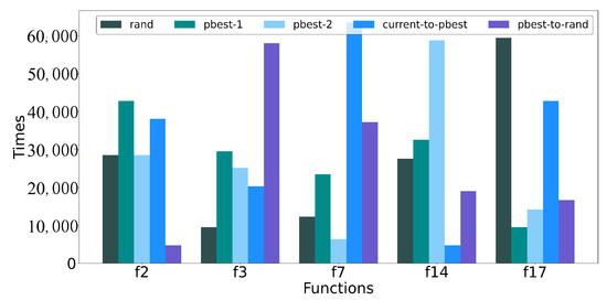
Figure 6. The frequency of strategies by function.

4.3. Comparison for CEC2013 Functions

In this section, we used the CEC2013 testing suite in experiment 2, to further illustrate the effectiveness of our algorithm SAABC-CS in handling complicated functions and high-dimensional issues. Since the CEC2013 test functions are more complicated than the 22 fundamental scalar functions, it was challenging to find the global best solution for CEC2013. We compared our algorithm SAABC-CS with the original ABC [12] and four additional cutting-edge ABC algorithms (ABCNG [33], KFABC [19], SABC-GB [15], and MGABC [30]). We measured the outcomes on D = 30, 50, and 100, to examine the comprehensive performance of these algorithms in several dimensions. For the fairness of the experiments, the methods were evaluated using the same parameters, SN = 100, limit = 1000, and MaxFEs = 10,000·D. The final statistical outcomes of the six related algorithms are encapsulated in Table 2, Table 3 and Table 4 based on 30 independent runs.

For D = 30, the results of the above ABC variations are reported in Table 2. For 21, 17, 25, 20, and 25 of the 28 test functions, our algorithm SAABC-CS outperformed or equaled the ABC, ABCNG, KFABC, SABC-GB, and MGABC in terms of outcomes. Additionally, SAABC-CS achieved the best results on 17 functions of F1–F5, F7, F8, F10, F12, F13, F15, F18, F20, F23-F25, and F28 when it was compared with the other algorithms. The statistical results of all algorithms on CEC2013 with the dimension D = 50 are shown in Table 3. SAABC-CS outperformed or equaled the ABC, ABCNG, KFABC, SABC-GB, and MGABC on 21, 17, 25, 20, and 25 out of 28 functions, respectively. The outcomes of all algorithms with the criterion D = 100 are displayed in Table 4. On 24, 20, 25, 19, and 25 out of 28 functions, SAABC-CS outperformed or equaled the ABC, ABCNG, KFABC, SABC-GB, and MGABC, with comparable or superior performance. Moreover, on F1–F9, F12–F13, F15–F20, F23–F25, and F28, SAABC-CS always achieved the best value out of all algorithms. As a result, SAABC-CS had the highest overall performance of the six algorithms that were examined.

To be more intuitive, we used the Friedman test [34] to rank all algorithms across all test problems, with the results shown in Table 5 and Figure 7. It is worth noting that the Friedman test uses the post hoc technique [35,36,37,38], and the lower the ranking, the better the overall performance of the algorithm. From the data, we can see the average rank of SAABC-CS was always the first for 30, 50, and 100 dimensions. Therefore, SAABC-CS’s effectiveness was always superior to the others on all dimensions.

Table 5. Average Ranking.

Function	D = 30	D = 50	D = 100
ABC	2.93	3.25	3.64
ABCNG	2.68	2.89	2.75
KFABC	5.20	5.32	5.00
SABC-GB	3.18	3.00	3.03
MGABC	3.50	3.42	3.57
SAABC-CS	2.17	2.07	1.92

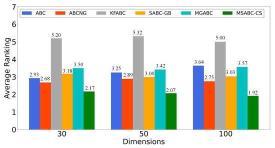
Figure 7. Illustration of Average Ranking.

We can further demonstrate the efficacy of our approach in finding the optimal for the complicated functions, based on the comparison findings mentioned above for the CEC2013 functions.

4.4. SAABC-CS for Practical Engineering Problems

In real-world engineering, parameter estimation of frequency-modulated (FM) sound waves [39] is frequently investigated. In this section, we performed tests to make comparisons between SAABC-CS and other ABC variants. We ran each algorithm 30 times independently and compared the results of the top outcomes of each algorithm.

4.4.1. Parameter Estimation for Frequency-Modulated (FM) Sound Waves

Frequency-modulated (FM) sound wave synthesis plays an important role in various modern music systems. To estimate the parameter of a FM synthesizer and to optimize the results, we solved a six-dimensional optimization problem, where we tried to optimize the vector $X=\{a_1,{\omega }_1,a_2,{\omega }_2,a_3,{\omega }_3\}$ given in Equation (19). The goal of this optimization problem was to generate a sound (19) similar to the target sound (20). This problem highly complex and multi-modal, having strong epistasis, with a minimum value $f\left(\overrightarrow{X_{sol}}\right)=0$. The expressions for the estimated sound and the target sound waves are given as

$$y\left(t\right)=a_1·sin({\omega }_1·t·\theta +a_2·sin({\omega }_2·t·\theta +a_3·sin({\omega }_3·t·\theta )\left)\right)$$

(19)

$$y_0\left(t\right)=1.0·sin(5.0·t·\theta -1.5·sin(4.8·t·\theta +2.0·sin(4.9·t·\theta )\left)\right)$$

(20)

where $\theta =(2·\pi )/100$ and the parameters are defined in the range $[-6.4,6.35]$. The fitness function is the summation of the square errors between the estimated wave (19) and the target wave (20), as follows:

$$minf\left(\overrightarrow{X}\right)={\displaystyle \sum _{t=0}^{100}}{(y\left(t\right)-y_0\left(t\right))}^2$$

(21)

4.4.2. Results of SAABC-CS Compared with Other Algorithms

Table 6 is a summary of the final results of our experiments, including the six parameters and the optimal cost. SAABC-CS obtained the minimum cost in solving the parameter estimation for frequency-modulated (FM) sound waves problem.

Table 6. SAABC-CS vs. other algorithms for parameter estimation of FM sound waves.

Algorithms	The Best Value of Six Parameters						Error Variance
	${\mathbf{a}}_{\mathbf{1}}$	${\mathbf{\omega }}_{\mathbf{1}}$	${\mathbf{a}}_{\mathbf{2}}$	${\mathbf{\omega }}_{\mathbf{2}}$	${\mathbf{a}}_{\mathbf{3}}$	${\mathbf{\omega }}_{\mathbf{3}}$
ABC	0.3559	0.0316	1.0678	0.1394	5.0670	4.9233	$1.659715\times {10}^1$
ABCNG	0.5546	0.0627	1.5207	0.1437	4.3253	4.9361	$1.460573\times {10}^1$
KFABC	0.1414	0.2657	0.1414	0.1414	0.1414	0.1414	$2.901492\times {10}^1$
MGABC	0.6894	14.6861	0.7746	9.7434	1.0506	5.1230	$1.226273\times {10}^1$
SABC-GB	0.7306	14.5462	0.6579	4.6106	5.7068	4.8736	$1.177162\times {10}^1$
SAABC-CS	0.3370	4.7477	0.4820	0.2280	1.2430	3.2447	$\mathbf{1}.\mathbf{024282}\times {\mathbf{10}}^{\mathbf{1}}$

5. Conclusions

In this paper, we proposed a new self-adaptive ABC algorithm with candidate strategies (SAABC-CS) to balance the exploration and exploitation of the evolution. Compared with the original ABC, SAABC-CS has three modifications, without adding any extra parameters: (1) five strategies are selected and assembled in a strategy pool; (2) a self-adaptive mechanism was designed to make the algorithm universal; (3) three neighbor mutations work together to enhance the scout phase. The aforementioned additions enhance ABC’s overall performance by allowing it to tackle complicated issues with more features, while balancing its exploration and development capabilities.

Comprehensive experiments were performed on two groups of functions: 22 basic benchmark functions and CEC2013 test suites. The experiment results for the 22 basic test functions showed that SAABC-CS obtained a much better performance than an ABC with one strategy. Furthermore, the self-adaptive selection mechanism in SAABC-CS was well-turned to select an appropriate strategy for facing problems of a different nature. For the complex and difficult CEC2013 benchmark suite, SAABC-CS still achieved promising results and surpassed four state-of-the-art ABCs. With the increasing dimensions of CEC2013, the performance of SAABC-CS did not deteriorate. The method also produced positive results when it was used to tackle real-world engineering challenges, demonstrating that it can solve real-world optimization problems as well as test functions.

Although extensive experiments were conducted to demonstrate the performance of SAABC-CS, we hope to theoretically analyze the algorithm, inspired by the literature [40,41,42]. We also wish to extend the use of SAABC-CS to certain large and expensive problems in the future.

References

- Whitley, D. A genetic algorithm tutorial. Stat. Comput. 1994, 4, 65–85. [Google Scholar] [CrossRef]
- Houck, C.R.; Joines, J.; Kay, M.G. A genetic algorithm for function optimization: A Matlab implementation. Ncsu-Ie Tr 1995, 95, 1–10. [Google Scholar]
- Wang, H.; Zhou, X.; Sun, H.; Yu, X.; Zhao, J.; Zhang, H.; Cui, L. Firefly algorithm with adaptive control parameters. Soft Comput. 2017, 21, 5091–5102. [Google Scholar] [CrossRef]
- Dorigo, M.; Birattari, M.; Stutzle, T. Ant colony optimization. IEEE Comput. Intell. Mag. 2006, 1, 28–39. [Google Scholar] [CrossRef]
- Qin, A.K.; Huang, V.L.; Suganthan, P.N. Differential evolution algorithm with strategy adaptation for global numerical optimization. IEEE Trans. Evol. Comput. 2008, 13, 398–417. [Google Scholar] [CrossRef]
- Qin, A.K.; Suganthan, P.N. Self-adaptive differential evolution algorithm for numerical optimization. In Proceedings of the 2005 IEEE Congress on Evolutionary Computation, Scotland, UK, 2–5 September 2005; Volume 2, pp. 1785–1791. [Google Scholar]
- Mallipeddi, R.; Suganthan, P.N.; Pan, Q.K.; Tasgetiren, M.F. Differential evolution algorithm with ensemble of parameters and mutation strategies. Appl. Soft Comput. 2011, 11, 1679–1696. [Google Scholar] [CrossRef]
- Kennedy, J.; Eberhart, R. Particle swarm optimization. In Proceedings of the ICNN’95—International Conference on Neural Networks, Perth, Australia, 27 November–1 December 1995; Volume 4, pp. 1942–1948. [Google Scholar]
- Shi, Y. Particle swarm optimization: Developments, applications and resources. In Proceedings of the 2001 Congress on Evolutionary Computation (IEEE Cat. No. 01TH8546), Seoul, Republic of Korea, 27–30 May 2001; Volume 1, pp. 81–86. [Google Scholar]
- Karaboga, D.; Basturk, B. On the performance of artificial bee colony (ABC) algorithm. Appl. Soft Comput. 2008, 8, 687–697. [Google Scholar] [CrossRef]
- Karaboga, D.; Akay, B. A comparative study of artificial bee colony algorithm. Appl. Math. Comput. 2009, 214, 108–132. [Google Scholar] [CrossRef]
- Karaboga, D. An Idea Based on Honey Bee Swarm for Numerical Optimization; Technical Report, Technical Report-tr06; Engineering Faculty, Erciyes University: Kayseri, Turkey, 2005. [Google Scholar]
- Bajer, D.; Zorić, B. An effective refined artificial bee colony algorithm for numerical optimisation. Inf. Sci. 2019, 504, 221–275. [Google Scholar] [CrossRef]
- Kumar, D.; Mishra, K. Co-variance guided artificial bee colony. Appl. Soft Comput. 2018, 70, 86–107. [Google Scholar] [CrossRef]
- Xue, Y.; Jiang, J.; Zhao, B.; Ma, T. A self-adaptive artificial bee colony algorithm based on global best for global optimization. Soft Comput. 2018, 22, 2935–2952. [Google Scholar] [CrossRef]
- Cui, L.; Li, G.; Zhu, Z.; Lin, Q.; Wen, Z.; Lu, N.; Wong, K.C.; Chen, J. A novel artificial bee colony algorithm with an adaptive population size for numerical function optimization. Inf. Sci. 2017, 414, 53–67. [Google Scholar] [CrossRef]
- Wang, H.; Wu, Z.; Rahnamayan, S.; Sun, H.; Liu, Y.; Pan, J.S. Multi-strategy ensemble artificial bee colony algorithm. Inf. Sci. 2014, 279, 587–603. [Google Scholar] [CrossRef]
- Gao, W.; Liu, S.; Huang, L. A novel artificial bee colony algorithm based on modified search equation and orthogonal learning. IEEE Trans. Cybern. 2013, 43, 1011–1024. [Google Scholar] [PubMed]
- Wang, H.; Wang, W.; Zhou, X.; Zhao, J.; Wang, Y.; Xiao, S.; Xu, M. Artificial bee colony algorithm based on knowledge fusion. Complex Intell. Syst. 2021, 7, 1139–1152. [Google Scholar] [CrossRef]
- Lu, R.; Hu, H.; Xi, M.; Gao, H.; Pun, C.M. An improved artificial bee colony algorithm with fast strategy, and its application. Comput. Electr. Eng. 2019, 78, 79–88. [Google Scholar] [CrossRef]
- Gao, W.; Liu, S. A modified artificial bee colony algorithm. Comput. Oper. Res. 2012, 39, 687–697. [Google Scholar] [CrossRef]
- Guo, P.; Cheng, W.; Liang, J. Global artificial bee colony search algorithm for numerical function optimization. In Proceedings of the 2011 Seventh International Conference on Natural Computation, Shanghai, China, 26–28 July 2011; Volume 3, pp. 1280–1283. [Google Scholar]
- Yu, W.J.; Zhan, Z.H.; Zhang, J. Artificial bee colony algorithm with an adaptive greedy position update strategy. Soft Comput. 2018, 22, 437–451. [Google Scholar] [CrossRef]
- Jadon, S.S.; Tiwari, R.; Sharma, H.; Bansal, J.C. Hybrid artificial bee colony algorithm with differential evolution. Appl. Soft Comput. 2017, 58, 11–24. [Google Scholar] [CrossRef]
- Alqattan, Z.N.; Abdullah, R. A hybrid artificial bee colony algorithm for numerical function optimization. Int. J. Mod. Phys. C 2015, 26, 1550109. [Google Scholar] [CrossRef]
- Chen, S.M.; Sarosh, A.; Dong, Y.F. Simulated annealing based artificial bee colony algorithm for global numerical optimization. Appl. Math. Comput. 2012, 219, 3575–3589. [Google Scholar] [CrossRef]
- Gao, W.f.; Huang, L.l.; Liu, S.y.; Chan, F.T.; Dai, C.; Shan, X. Artificial bee colony algorithm with multiple search strategies. Appl. Math. Comput. 2015, 271, 269–287. [Google Scholar] [CrossRef]
- Song, X.; Zhao, M.; Xing, S. A multi-strategy fusion artificial bee colony algorithm with small population. Expert Syst. Appl. 2020, 142, 112921. [Google Scholar] [CrossRef]
- Chen, X.; Tianfield, H.; Li, K. Self-adaptive differential artificial bee colony algorithm for global optimization problems. Swarm Evol. Comput. 2019, 45, 70–91. [Google Scholar] [CrossRef]
- Zhou, X.; Lu, J.; Huang, J.; Zhong, M.; Wang, M. Enhancing artificial bee colony algorithm with multi-elite guidance. Inf. Sci. 2021, 543, 242–258. [Google Scholar] [CrossRef]
- Zhu, G.; Kwong, S. Gbest-guided artificial bee colony algorithm for numerical function optimization. Appl. Math. Comput. 2010, 217, 3166–3173. [Google Scholar] [CrossRef]
- Mühlenbein, H.; Schomisch, M.; Born, J. The parallel genetic algorithm as function optimizer. Parallel Comput. 1991, 17, 619–632. [Google Scholar] [CrossRef]
- Xiao, S.; Wang, H.; Wang, W.; Huang, Z.; Zhou, X.; Xu, M. Artificial bee colony algorithm based on adaptive neighborhood search and Gaussian perturbation. Appl. Soft Comput. 2021, 100, 106955. [Google Scholar] [CrossRef]
- Derrac, J.; García, S.; Molina, D.; Herrera, F. A practical tutorial on the use of nonparametric statistical tests as a methodology for comparing evolutionary and swarm intelligence algorithms. Swarm Evol. Comput. 2011, 1, 3–18. [Google Scholar] [CrossRef]
- Wang, B.C.; Li, H.X.; Li, J.P.; Wang, Y. Composite differential evolution for constrained evolutionary optimization. IEEE Trans. Syst. Man, Cybern. Syst. 2018, 49, 1482–1495. [Google Scholar] [CrossRef]
- Wang, Y.; Li, J.P.; Xue, X.; Wang, B.C. Utilizing the correlation between constraints and objective function for constrained evolutionary optimization. IEEE Trans. Evol. Comput. 2019, 24, 29–43. [Google Scholar] [CrossRef]
- Wang, Y.; Wang, B.C.; Li, H.X.; Yen, G.G. Incorporating objective function information into the feasibility rule for constrained evolutionary optimization. IEEE Trans. Cybern. 2015, 46, 2938–2952. [Google Scholar] [CrossRef]
- Fan, Q.; Jin, Y.; Wang, W.; Yan, X. A performancE—driven multi-algorithm selection strategy for energy consumption optimization of sea-rail intermodal transportation. Swarm Evol. Comput. 2019, 44, 1–17. [Google Scholar] [CrossRef]
- Das, S.; Suganthan, P.N. Problem Definitions and Evaluation Criteria for CEC 2011 Competition on Testing Evolutionary Algorithms on Real World Optimization Problems; Jadavpur University, Nanyang Technological University: Kolkata, India, 2010; pp. 341–359. [Google Scholar]
- KhalafAnsar, H.M.; Keighobadi, J. Adaptive Inverse Deep Reinforcement Lyapunov learning control for a floating wind turbine. Sci. Iran. 2023, in press. [Google Scholar] [CrossRef]
- Keighobadi, J.; KhalafAnsar, H.M.; Naseradinmousavi, P. Adaptive neural dynamic surface control for uniform energy exploitation of floating wind turbine. Appl. Energy 2022, 316, 119132. [Google Scholar] [CrossRef]
- Keighobadi, J.; Nourmohammadi, H.; Rafatania, S. Design and Implementation of GA Filter Algorithm for Baro-inertial Altitude Error Compensation. In Proceedings of the Conference: ICLTET-2018, Istanbul, Turkey, 21–23 March 2018; pp. 21–23. [Google Scholar]
Disclaimer/Publisher’s Note: The statements, opinions and data contained in all publications are solely those of the individual author(s) and contributor(s) and not of MDPI and/or the editor(s). MDPI and/or the editor(s) disclaim responsibility for any injury to people or property resulting from any ideas, methods, instructions or products referred to in the content. |
© 2023 by the authors. Licensee MDPI, Basel, Switzerland. This article is an open access article distributed under the terms and conditions of the Creative Commons Attribution (CC BY) license (https://creativecommons.org/licenses/by/4.0/).