Abstract
This paper secures solitary waves and conservation laws to the familiar Korteweg–de Vries equation and Gardner’s equation with three dispersion sources. The traveling wave hypothesis leads to the emergence of such waves. The three sources of dispersion are spatial dispersion, spatio–temporal dispersion and the dual-emporal–spatial dispersion. The conservation laws are enumerated for these models, evolved from the multiplier approach. The conserved quantities are computed with the solitary wave solutions that were recovered.
1. Introduction
One of the several forms of pre–existing models for shallow water waves is the Korteweg–de Vries (KdV) equation, which has been extensively investigated [1,2,3,4,5,6,7,8,9,10,11,12,13,14,15,16,17,18,19,20]. A deluge of results has appeared from a variety of sources, ranging from its integrability, numerical schemes, and vector forms of the model for addressing multi-layered flow. The KdV equation was handled with various forms of nonlinearity, including arbitrary power–law. The model was also addressed with logarithmic law of nonlinearity, which yielded Gaussian solitary waves [3]. Later, multi-layered fluid flow along lake–shores and beaches was studied with the Gear–Grimshaw model as well as the Zareamoghaddam model, which were successfully handled both analytically and numerically together with the recovery of solitary wave solutions and their conservation laws [2,3,6]. Subsequently, the KdV equation was extended/generalized to incorporate dual nonlinear effects. This is Gardner’s equation (GE), which was later studied extensively to address shallow water wave effects. It is not out of place to point out the fact that apart from the KdV equation and Gardner’s equation, there are several other forms of nonlinear wave equations that gave way to N–soliton solutions. The method of integrability for such models is the Riemann–Hilbert approach. although there is yet another well-known and well-established scheme to locate N–soliton solutions including soliton radiation [11,12,13]. This is the Inverse Scattering Transform (IST).
The current paper will revisit both models with the inclusion of triple dispersive effects that stem from triple spatial dispersion, spatio–temporal dispersion and dual-temporal–spatial dispersion. This gives an extension to the familiar couple of models that have been studied with third-order dispersion only. While the spatio–temporal dispersion is addressed in shallow water waves with Benjamin–Bona–Mahoney equation, the dual-temporal-spatial dispersive effect was first proposed in 1977 by Joseph and Egri and was never seen again after its first appearance [4]. The current work incorporates all three dispersive effects, and the solitary waves for both models are recovered. The relation between the inverse width and the soliton velocity are also analyzed. The simulations finally led to the visual effect of behind-the-scenes, mathematical analysis of the models. The conservation laws for all models are exhibited as well.
Governing Model
The generalized form of the KdV equation and its type are all incorporated in the following structure:
Here, and are the independent variables that respectively depict spatial and temporal variables. Then, the dependent variable represents the wave profile. The first term is the temporal evolution of the wave. The second term is from the effect of nonlinearity, which contains a single effect for the KdV equation and dual nonlinear terms that give GE. The three dispersion terms carry the coefficients for , from triple spatial dispersion, spatio–temporal dispersion, and dual-temporal–spatial dispersion effects, respectively. The KdV equation and GE has , which has exhausted the journals [1,3,5,7,16].
In order to study the model expressed by Equation (1) with traveling wave hypothesis, one would choose the following hypothesis:
Here, the function denotes the solitary wave profile, with being the velocity of the wave. This assumption would transform (1) into the following ordinary differential equation (ODE):
which itegrates to
upon choosing the integration constant to be zero, as relevant for solitary waves. Next, multiplying (3) by and integrating leads to
The final integration that would lead to the solitary wave solution would be possible once the exact form of nonlinearity is considered. This study would therefore be classified into the subsequent three subsections depending on the type of nonlinearity.
The study will be split into two sections that detail the KdV equation and GE in sequence. The first section contains three subsections based on the structure of the nonlinear term while the second section has two subsections based on the structure of the two nonlinear terms. The details on traveling waves and the conservation laws are also extracted.
2. Single Nonlinearity (KdV Equations)
Equation (1) will now be studied with a single nonlinear term of three different types. The traveling wave hypothesis will lead to the solitary waves to be derived, and the corresponding parameter constraints will be enlisted for all three cases. The respective conservation laws will be retrieved by the multiplier method, and the conserved quantities will be computed using the derived solitary wave solution.
2.1. KdV Equation
For this model, for any real-valued constant . From (1), this leads to [4]
which would mean that (5) transforms into
Finally, separating variables and integrating yields a solitary wave solution as follows:
Here, the inverse width is and is the amplitude of the wave; they are presented below as
and
The width of the wave therefore introduces the following parameter constraint:
Figure 1 depicts the surface plot of a solitary wave (8) of the KdV equation with triple dispersion terms. The parameter values chosen are , , , , and .
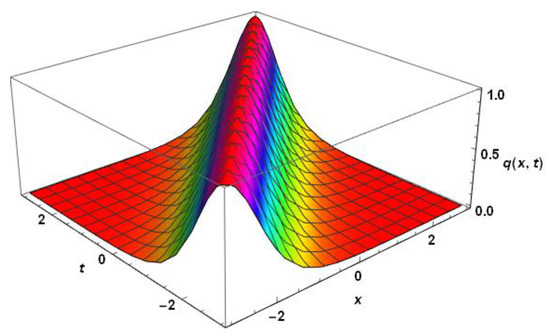
Figure 1.
Profile of a solitary wave for the KdV equation, without radiation.
Conservation Laws
For the conserved flow that renders a closed form of the respective models, satisfies along the solutions. represents the conserved density and is the conserved flux [2,4,5,9,14,15]. We present the various densities that arise from the multipliers when
Case 1:
Case 2:
Case 3:
and
Therefore, the respective conserved quantities are
and
Here, gives the Hamiltonian, stems from linear momentum, and is from mass. To evaluate the integrals in (17)–(19), the solitary wave solution given by (8) is utilized.
2.2. Modified KdV Equation
Here, for any real-valued constant . From (1), this leads to [8]
which means that (5) transforms into
Thus, Equation (20) is the generalization of Equation (6) for the mKdV equation with the dispersion triplet. This is also the generalized version of the KdV equation that was first proposed during 1977 [8]. Finally, separating variables and integrating yields a solitary wave solution as follows:
Here, the inverse width is and is the amplitude of the wave; they are defined as
and
which would once again imply the parameter constraint as given by (11). This time, the amplitude of the solitary wave imposes the restriction
Figure 2 displays the surface plot of a solitary wave (22) of the mKdV equation with triple dispersion terms. The parameter values chosen are , , , , and .
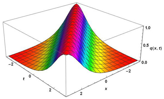
Figure 2.
Profile of a solitary wave for the mKdV equation, without radiation.
Conservation laws
In this case, the multipliers, conserved densities, and fluxes are given as
Case 1:
Case 2:
Case 3:
and
Thus, for mKdV equation, the conserved quantities are
2.3. Power–Law KdV Equation
Now, for any real-valued constant . From (1), this leads to
which means that (5) transforms into
Finally, separating variables and integrating yields a solitary wave solution as follows:
Here, the inverse width is and is the amplitude of the wave; they are indicated below as
and
which would once again imply the parameter constraint as given by (11). Figure 3 indicates the surface plot of a solitary wave (35) of the power–law KdV equation with triple dispersion terms with . The parameter values chosen are , , , , and .
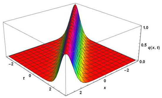
Figure 3.
Profile of a solitary wave for the power–law KdV equation, without radiation.
Conservation Laws
For the power–law KdV equation, the multipliers, densities, and fluxes are given as
Case 1:
Case 2:
Case 3:
and
For power–law, the conserved quantities are
and
3. Dual-Nonlinearity (Gardner’s Equation)
This section studies Equation (1), which carries two nonlinear terms and is typically referred to as Gardner’s equation, alternatively known as the KdV–mKdV equation. The dispersion triplet remains. The two subsections study Gardner’s equation and its generalization to power–law nonlinearity. In each of these subsections, the traveling wave hypothesis would yield the solitary wave solutions along with the corresponding conservation laws that are derived using the multiplier approach.
3.1. KdV–mKdV Equation
Here, for any real-valued constants for . From (1), this leads to [8]
which means that (5) transforms into
Equation (45) is the familiar KdV–mKdV equation that is here being addressed with three sources of dispersion for the first time. This equation was studied in the past, but only with spatial dispersion, using the semi-inverse variational principle [8]. Finally, separating variables and integrating yields a solitary wave solution as follows:
Here, the inverse width is with an external parameter , while is the amplitude of the wave. The amplitude can be expressed as
and the inverse width is the same as (10). The parameter is given as
The inverse width and the parameter pose the constraint
Figure 4 depicts the surface plot of a solitary wave (47) of Gardner’s equation with triple dispersion terms. The parameter values chosen are , , , , , and .
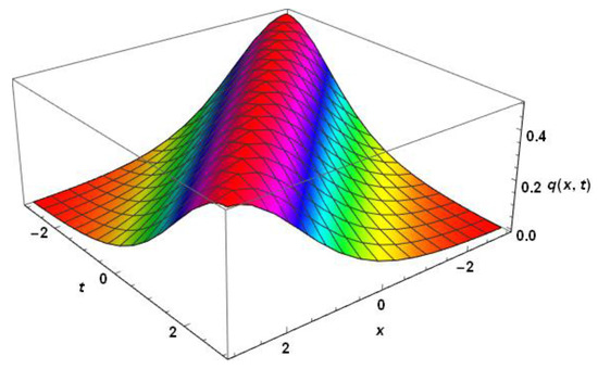
Figure 4.
Profile of a solitary wave for Gardner’s equation without radiation.
Conservation Laws
Here, the multipliers, densities, and the fluxes are
Case 1:
Case 2:
Case 3:
and
For Gardner’s equation, the three conserved quantities are
and
where in (55)–(57), the Gauss’ hypergeometric function is indicated below as [1]
with the Pochhammer symbol being
The convergence of the series is defined provided
which translates to
Finally, Rabbe’s test of convergence yields the convergence criterion
which is valid for (55)–(57).
3.2. Power–Law Nonlinearity
Here, for any real-valued constant . From (1), this leads to
which means that (5) transforms into
Finally, separating variables and integrating yields a solitary wave solution as follows:
Here, the inverse width is with an external parameter , while is the amplitude of the wave. The amplitude is introduced below as
while the inverse width is
which poses the same constraint as in (11). The parameter is given as
The inverse width and the parameter must maintain the condition
for the solitary waves to exist. Figure 5 displays the surface plot of a solitary wave (65) for the power–law Gardner’s equation with triple dispersion terms with . The parameter values chosen are , , , , , and .
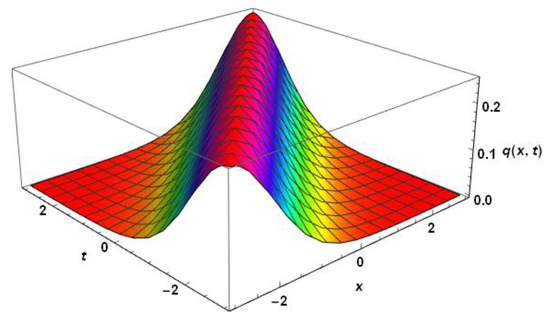
Figure 5.
Profile of a solitary wave for the power–law Gardner’s equation, without radiation.
Conservation Laws
Here, the multipliers, densities, and fluxes are
Case 1:
Case 2:
Case 3:
The corresponding conserved density and flux are too cumbersome to construct. The first two conservation laws are
and
4. Conclusions
The current work recovered solitary wave solutions to the KdV and Gardner’s equation, appearing with algebraic-type nonlinearities. The two model equations carry three forms of dispersion that are a combination of spatial and temporal types. The novelty of the work is the inclusion of these three forms of dispersion, yielding different relations for the amplitude and inverse width of the wave with its velocity. These results collapse to the pre-existing results that appear with third-order spatial dispersion only. The conservation laws are also computed for both models with all forms of nonlinearity addressed in the present paper. One of the inherent shortcomings of the traveling waves hypothesis approach to retrieve solitary waves is its failure to retrieve soliton radiation. This is only achievable with the usage of IST, which is outside the scope of the current work.
Thus, these results pave the way for several new avenues. In the future, the model would be studied with transcendental nonlinearities, and the perturbation terms would be included to address the models from an advanced standpoint. Such works would include the application of the semi-inverse variational algorithms, the application of soliton perturbation theory, and the study of multi-layered fluid flow, not to mention handling the models numerically with the application of the Laplace–Adomian scheme, the variational iteration approach, and others. These research works are very much anticipated and will be presented in succession.
Author Contributions
Conceptualization, A.B. and N.C.; methodology, A.H.K. and S.K.; software, Y.Y.; writing—original draft preparation, S.M.; writing—review and editing, C.I.; project administration, L.M. All authors have read and agreed to the published version of the manuscript.
Funding
This research received no external funding.
Institutional Review Board Statement
Not applicable.
Informed Consent Statement
Not applicable.
Data Availability Statement
Not applicable.
Acknowledgments
The authors thank the anonymous referees whose comments helped to improve the paper.
Conflicts of Interest
The authors declare no conflict of interest.
References
- Antonova, M.; Biswas, A. Adiabatic parameter dynamics of perturbed solitary waves. Commun. Nonlinear Sci. Numer. Simul. 2009, 14, 734–748. [Google Scholar] [CrossRef]
- Biswas, A.; Kara, A.H. 1–soliton solution and conservation laws for nonlinear wave equation in semiconductors. Appl. Math. Comput. 2010, 217, 4289–4292. [Google Scholar] [CrossRef]
- Biswas, A.; Ismail, M.S. 1–soliton solution of the coupled KdV equation and Gear–Grimshaw model. Appl. Math. Comput. 2010, 216, 3662–3670. [Google Scholar] [CrossRef]
- Biswas, A.; Krishnan, E.V.; Suarez, P.; Kara, A.H.; Kumar, S. Solitary waves and conservation laws of Bona—Chen equation. Indian J. Phys. 2013, 87, 169–175. [Google Scholar] [CrossRef]
- Collins, T.; Kara, A.H.; Bhrawy, A.H.; Triki, H.; Biswas, A. Dynamics of shallow water waves with logarithmic nonlinearity. Rom. Rep. Phys. 2016, 68, 943–961. [Google Scholar]
- Gepreel, K.A. Exact soliton solutions for nonlinear perturbed Schrödinger equations with nonlinear optical media. Appl. Sci. 2020, 10, 8929. [Google Scholar] [CrossRef]
- Girgis, L.; Biswas, A. A study of solitary waves by He’s semi–inverse variational principle. Waves Random Complex Media 2011, 21, 96–104. [Google Scholar] [CrossRef]
- Joseph, R.I.; Egri, R. Another possible model equation for long waves in nonlinear dispersive system. Phys. Lett. A 1977, 61, 429–430. [Google Scholar] [CrossRef]
- Khan, S. Conservation laws of Biswas–Arshed equation in optical fibers (filling in the gap). Optik 2019, 194, 163037. [Google Scholar] [CrossRef]
- Kudryashov, N.A. A note on solutions of the Korteweg–de Vries hierarchy. Commun. Nonlinear Sci. Numer. Simul. 2011, 16, 1703–1705. [Google Scholar] [CrossRef]
- Ma, W. Riemann–Hilbert problems and soliton solutions of nonlocal reverse-time NLS hierarchies. Acta Math. Sci. 2022, 42, 127–140. [Google Scholar] [CrossRef]
- Ma, W. Riemann–Hilbert problems and inverse scattering of nonlocal real reverse--spacetime matrix AKNS hierarchies. Phys. D 2022, 430, 133078. [Google Scholar] [CrossRef]
- Ma, W. Riemann–Hilbert problems and soliton solutions of type (,) reduced nonlocal integrable mKdV hierarchies. Mathematics 2022, 10, 870. [Google Scholar] [CrossRef]
- Masemola, P.; Kara, A.H.; Bhrawy, A.H.; Biswas, A. Conservation laws for coupled wave equations. Rom. J. Phys. 2016, 61, 367–377. [Google Scholar]
- Krishnan, E.V.; Kara, A.H.; Kumar, S.; Biswas, A. Topological solitons, cnoidal waves and conservation laws of coupled wave equations. Indian J. Phys. 2013, 87, 1233–1241. [Google Scholar] [CrossRef]
- Triki, H.; Kara, A.H.; Bhrawy, A.; Biswas, A. Soliton solutions and conservation laws for Gear–Grimshaw model for shallow water waves. Acta Phys. Pol. A 2014, 125, 1099–1106. [Google Scholar] [CrossRef]
- Wazwaz, A.M. Analytic study on the generalized fifth–order KdV equation: New solitons and periodic solutions. Commun. Nonlinear Sci. Numer. Simul. 2007, 12, 1172–1180. [Google Scholar] [CrossRef]
- Wazwaz, A.M. Integrability of coupled KdV equations. Cent. Eur. J. Phys. 2011, 9, 835–840. [Google Scholar] [CrossRef]
- Wazwaz, A.M. New (3+1)–dimensional nonlinear equations with KdV equation constituting its main part: Multiple soliton solutions. Math. Methods Appl. Sci. 2016, 39, 886–891. [Google Scholar] [CrossRef]
- Wazwaz, A.M. Multiple soliton solutions and other exact solutions for a two–mode KdV equation. Math. Methods Appl. Sci. 2016, 40, 2277–2283. [Google Scholar] [CrossRef]
Publisher’s Note: MDPI stays neutral with regard to jurisdictional claims in published maps and institutional affiliations. |
© 2022 by the authors. Licensee MDPI, Basel, Switzerland. This article is an open access article distributed under the terms and conditions of the Creative Commons Attribution (CC BY) license (https://creativecommons.org/licenses/by/4.0/).