An Overview of the Seismic Elastic Response Spectra and Their Application According to Mexican, U.S., and International Building Codes

Abstract

The design of earthquake-resistant structures by applying traditional or performance-based seismic analysis methods involves two large variables: the seismic risk of the area and the physical characteristics of the structure. Before analyzing any building, it is required to determine the seismicity in the location to evaluate the accelerations that the structure must withstand by deterministic or probabilistic methods. The typical results of a seismic study are the uniform hazard spectra in the rock layer related to a specific return period and structural damping. The building codes use different methods to obtain the elastic response spectra, seeking to offer simple procedures by using parametric factors to consider the soil type; however, the procedure tends to return conservative estimates. On the other hand, site-specific spectra offer accurate and less conservative acceleration values, with the disadvantage of an extensive and costly mathematical process, justifying their application mostly to important structures. This review article gives the state of the art of seismic elastic response spectra using probabilistic seismic hazard maps as inputs, taking into account the importance of the structure and the soil type, according to Mexican, U.S., and international building codes.

1. Introduction

Seismic response spectra and their application to any structure require knowledge of the seismicity at the location, the geological fault types, the path of the measured seismic waves from the focus to the site of interest, and the attenuation of the wave amplitudes through the Earth’s crust. The result of the study is the uniform seismic hazard spectra in a rock layer, represented as a graph of accelerations vs. structural periods, related to a specific return period.

Spectral accelerations in a rock layer are used to create seismic hazard maps and regionalization of seismic zones, which are the initial inputs required to obtain the elastic seismic spectrum. To consider site effects due to soft soils, the dynamic amplification factors must be analyzed according to the physical characteristics of the soil in the site of interest, taking into account the stiffness difference between the rock and soft soil layers.

Many countries have seismic hazard maps incorporated in their building codes, applying the probabilistic approach according to the seismic engineering methods. In addition, these codes allow for the analysis of a specific earthquake with a deterministic approach for special cases, such as earthquakes of very high magnitude applied to structures of high importance.

With the seismic hazard maps and the soil mechanics studies at the site of interest available, including the dynamic properties of the soil, an elastic response spectrum can be obtained, showing, as a result, the spectral accelerations for many structural periods. Its application is directly related to the study of buildings’ behavior under different seismic loads. Therefore, it is important to define all the parameters to obtain the seismic intensities and propose structural solutions to adequately support these seismic loads.

There are several methods of structural analysis and design that are used to evaluate the displacements and stresses in a building under seismic loads where the force and displacement methods are the most common. The force-based method determines the seismic loads and applies them to the structure to obtain the stresses and displacements on each element. On the other hand, the displacement-based method shows results as global displacements in the first step and, thus, obtains the strain and stresses on each individual element. Traditional seismic engineering and performance-based seismic engineering can use any force-based or displacement-based methods, applying the seismic response spectra as an external load input.

National and international building codes establish the minimum requirements for earthquake-resistant structures, including the procedures to obtain the elastic response spectrum and the design spectrum, where the latter depends on different reduction factors according to the characteristics of each building. Mexico has the Design Manual for Civil Works, Seismic Design (in Spanish, Manual de Diseño de Obras Civiles, Diseño por Sismo), developed by the Comision Federal de Electricidad, or MDOC Sismo CFE 2015 [1]; the USA has the American Society of Civil Engineers/Structural Engineering Institute or ASCE/SEI 7-16 [2]. For international reference, the International Building Code or IBC 2018 [3] is used. There are more local and international codes that have similar methodologies, showing the procedures to obtain the spectral acceleration in rock layers according to the country’s seismic hazard maps.

This review article will provide an overview of the methods developed by Mexico, the USA, and IBC to obtain the seismic elastic response spectra according to the seismic hazard variables. The process includes the constant acceleration, regional spectra, and site-specific response spectra procedures, considering as inputs the spectral accelerations in rock layers related to a probabilistic approach. The seismic spectrum obtained with a deterministic approach is mentioned as a global method, since it requires the local seismicity, the distance from the seismic source to the site of interest, and the attenuation of the seismic waves using the ground motion prediction equations (GMPE). Finally, the seismic spectrum named acceleration displacement response spectra (ADRS) with $S_d \mathrm{vs}. S_a$ format, used in performance-based seismic engineering, is shown.

2. Criteria for Seismic Elastic Response Spectra

There are two criteria used to obtain the seismic elastic response spectra at the site of interest: the descriptive method and the calculated method. The descriptive method follows the equations established by the different seismic codes to obtain seismic elastic response spectra, using as inputs the rock acceleration from the seismic hazard maps and the ground fundamental vibration period. The calculated method uses the same seismic hazard maps to create simulations of compatible synthetic accelerograms, applying all dynamic properties of the soil layers, either by equations or by modeling using a finite element method (FEM) procedure.

The seismic codes of each country contain the seismic hazard maps according to the probabilistic approach, offering the elastic response spectra in rock layers without any type of modification, either by soil characteristics or by the nature of the structure. In the following sections, the procedure to obtain the seismic elastic response spectra are reviewed according to MDOC Sismo CFE 2015 [1], ASCE/SEI 7-16 [2], and IBC 2018 [3].

3. Seismic Response Spectra in Mexico

According to MDOC Sismo CFE 2015 [1], a seismic hazard map for Mexico is presented with a scale of maximum accelerations in the rock layer according to the probabilistic seismic hazard study, as shown in Figure 1. The map shows zones with high spectral acceleration values in a dark blue color, which corresponds to the subduction fault in the southern side of the country and the transcurrent fault in the peninsula area of Baja California. The objective of the map is to provide the rock acceleration as initial input showing the Reference Spectrum graph, or in Spanish, Espectro de Referencia (ER), used to obtain the seismic elastic response spectrum. The map does not show a specific return period, $T_r$, since an optimal design is considered depending on the expected losses in the buildings after the seismic event, taking into account the economic aspect.

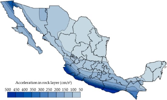
Figure 1. Maximum acceleration in the rock layer used for the reference spectrum ER, reproduced with permission from Ulises Mena, Comisión Federal de Electricidad Manual de Diseño de Obras Civiles; published by Comision Federal de Electricidad (CFE), 2015 [1].

In order to simplify the levels of seismic hazard, Figure 2 shows the seismic zones classification and Table 1 contains the spectral values in rock according to each seismic zone, where zone A corresponds to areas with low seismic hazard and zone D corresponds to high seismic hazard, matching the acceleration values in Figure 1.

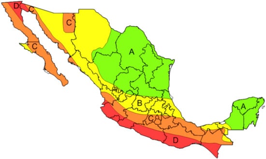
Figure 2. Seismic hazard zones classification in Mexico, reproduced with permission from Ulises Mena, Comisión Federal de Electricidad Manual de Diseño de Obras Civiles; published by Comision Federal de Electricidad (CFE), 2015 [1].

Table 1. Maximum acceleration, velocity, and displacement in the rock layer for each seismic zone, adapted with permission from Ulises Mena, Comisión Federal de Electricidad Manual de Diseño de Obras Civiles; published by Comision Federal de Electricidad (CFE), 2015 [1].

Zone	$\mathbf{Maximum}\mathbf{Acceleration}\mathbf{in}\mathbf{Rock},{\mathit{a}}_{0\mathit{r}} {\left(cm/s^2\right)}^1$	$\mathbf{Maximum}\mathbf{Velocity}\mathbf{in}\mathbf{Rock},{\mathit{v}}_{\mathit{r}\_\mathit{m}\mathit{a}\mathit{x}} {\left(cm/s\right)}^2$	$\mathbf{Maximum}\mathbf{Displacement}\mathbf{in}\mathbf{Rock},{\mathit{d}}_{\mathit{r}\_\mathit{m}\mathit{a}\mathit{x}} {\left(cm\right)}^2$	Seismic Intensity
A	$a_{0r}\le 50$	$4\le v_{r\_max}<10$	$1\le d_{r\_max}\le 21$	Low
B	$50\le a_{0r}<100$	$6\le v_{r\_max}<18$	$6\le d_{r\_max}<50$	Moderate
C	$100\le a_{0r}<200$	$11\le v_{r\_max}<27$	$6\le d_{r\_max}<50$	High
D	$a_{0r}\ge 200$	$21\le v_{r\_max}<62$	$35\le d_{r\_max}<99$	Very high

¹ The maximum acceleration in the rock layer, $a_{0r}$ corresponds to the reference spectrum ER used to obtain the seismic elastic spectra. ² The maximum velocity, $v_{r\_max}$, and the maximum displacement, $d_{r\_max}$, in the rock layer correspond to the reference spectrum ER and depend on the site location in the seismic hazard map using PRODISIS software [4].

Table 1 shows the spectral acceleration values in the rock layer related to each seismic zone, scaling the seismic intensities from low to very high. Values greater than $200 \mathrm{cm}/{\mathrm{s}}^2$ correspond to a very high seismic intensity with zone D classification.

3.1. Initial Inputs for the Elastic Design Spectrum According to MDOC Sismo CFE 2015

For the seismic elastic design spectrum, it is required to know the importance of the structure, the reference spectrum ER in the rock layer, and the soil physical properties, which include the dynamic amplification factors due to the site effects.

The first step would be defining the importance of the structure, assigning a group and/or subgroup according to Table 2, which depends on the occupancy of the building. Group A+ contains buildings of great importance that require a very high safety level in the presence of a strong earthquake, where the failure can be related to major environmental or economic disasters. Group A refers to structures of high importance that require a high safety level, and group B includes all other ordinary structures with moderate safety level. Buildings related to the energy sector are classified within groups A+ and A, while ordinary structures such as offices, houses, and industrial buildings are classified within group B.

Table 2. Importance of buildings and their requirements related to the elastic design spectrum, adapted with permission from Ulises Mena, Comisión Federal de Electricidad Manual de Diseño de Obras Civiles; published by Comision Federal de Electricidad (CFE), 2015 [1].

Group	Description	Building Examples	Subgroup	Building Classification
A+	Structures of great importance	Dams and nuclear plants	--	Energy or industrial sector of great importance
A	Structures with high safety level	Electric power generators, bridges, water treatment plants, and buildings	A1	Belong to the energy or industrial sector
			A2	Do not belong to the energy or industrial sector
B	Structures with ordinary safety level	Industrial buildings, offices, houses, and other common structures	B1	Buildings with height $H>13 \mathrm{m}$ or built area $A>400 {\mathrm{m}}^2$
			B2	Buildings with height $H\le 13 \mathrm{m}$ and or built area $A\le 400 {\mathrm{m}}^2$

By selecting the group and/or subgroup according to the structure’s importance, three variables can be defined: the structural importance factor, $F_{IE}$, the seismic elastic design spectra procedure, and the soil dynamic properties data of the site.

The structural importance factor, $F_{IE}$, is applied directly to the spectrum by multiplying the acceleration values to ensure structural safety. The seismic elastic design spectra procedure can be classified into three types: constant acceleration spectra, regional spectra, and site-specific spectra. The soil dynamic properties of the site show the required data from the soil layers to obtain different solutions, either numerically or mathematically. Therefore, the above three factors depend on the group and/or subgroup.

Table 3 shows the different seismic elastic design spectrum procedures to be used, according to the group and/or subgroup selected, where the structural importance factor, $F_{IE}$, and the soil dynamic analysis have different combinations.

Table 3. Spectra types, importance factors, and soil properties for each group and subgroup, adapted with permission from Ulises Mena, Comisión Federal de Electricidad Manual de Diseño de Obras Civiles; published by Comision Federal de Electricidad (CFE), 2015 [1].

Group	Sub Group	Soil Data	Soil Dynamic Analysis	Spectrum Type in Rock Layer 1	Elastic Design Spectrum Type	FIE
A+	--	Soil study by layers, topography and dynamic properties	Dynamic analysisby finite elementsor similar methods	Probabilistic spectrum with a specific return period, $T_r$, called return period reference spectrum (EPR)	Site-specific spectrum	1.0
				Deterministic spectrum for a maximum considered earthquake (MCE), less than a probabilistic spectrum with $T_r=\mathrm{10,000} \mathrm{years}$	Site-specific spectrum	1.0
				Probabilistic reference spectrum (ER)	Site-specific spectrum	1.75
A	A1	Soil study by layers and dynamic properties	Analysis of soil transfer functions	Probabilistic spectrum with a specific return period, $T_r$, called return period reference spectrum (EPR)	Site-specific spectrum	1.0
				Deterministic spectrum for a maximum considered earthquake (MCE), less than a probabilistic spectrum with $T_r=2475 \mathrm{years}$	Site-specific spectrum	1.0
				Probabilistic reference spectrum (ER)	Site-specific spectrum	1.5
	A2	Soil study by layers and shear wave velocity	Fundamental vibration period	Probabilistic reference spectrum (ER)	Regional spectrum	1.5
B	B1	Soil study by layers and shear wave velocity	Fundamental vibration period	Probabilistic reference spectrum (ER)	Regional spectrum	1.0
	B2	Not required	Not required	Probabilistic reference spectrum (ER)	Constant acceleration spectrum	1.0

¹ For A+ and A groups, any seismic spectrum type can be selected for the envelope.

According to Table 3, the structures of subgroup B2 have been assigned the constant acceleration spectrum, where the soil studies are not required due to the limited budget of small projects, simplifying the spectral acceleration procedure but with the disadvantage of conservative results. For subgroups B1 and A2, the structures have been assigned the regional spectrum, using a basic soil study to obtain the fundamental vibration period. For subgroups A1 and A+, the buildings have been assigned the site-specific spectrum, which requires a detailed soil study of the site to obtain data related to the dynamic properties.

The spectral accelerations in the rock layer at the site of interest can be obtained using the PRODISIS program, developed by the Comision Federal de Electricidad, where the probabilistic seismic hazard map of Mexico is shown [4]. The software contains the mapped seismic spectral acceleration in the rock layer, requiring the location of the structure as input, and the program will show the acceleration graph and named reference spectrum ER with an optimal return period, $T_r$. In addition, the software allows us to modify the return period using a specific value, where the spectral acceleration values will be adjusted, showing a graph called return period reference spectrum, or in Spanish, Espectro de Referencia a un Periodo de Retorno (EPR).

Figure 3 shows an example of PRODISIS response spectra results, where the city of Puebla is located on the map and the software automatically displays the reference spectrum (ER) with an optimal return period of $T_r=408 \mathrm{years}$, showing in blue color the maximum spectral acceleration in a rock layer of $391\mathrm{cm}/{\mathrm{s}}^2$ at a structural period of $T_e=0.15 \mathrm{s}$. Additionally, a return period reference spectrum (EPR) is obtained using a return period value of $T_r=975 \mathrm{years}$, where the software displays the graph of spectral accelerations in green with a maximum spectral acceleration in the rock layer of $588\mathrm{cm}/{\mathrm{s}}^2$ at a structural period of $T_e=0.15 \mathrm{s}$.

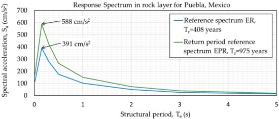
Figure 3. Seismic spectra results obtained from PRODISIS software for the city of Puebla, Mexico.

The constant acceleration spectrum, regional spectrum, and site-specific spectrum are procedures available to obtain the seismic elastic design spectrum according to Table 3. Therefore, the following sections explain the steps used to obtain the seismic elastic spectral accelerations using each of the three procedures, taking into account the dynamic amplification factors of the site.

3.2. Constant Acceleration Spectrum According to MDOC Sismo CFE 2015

According to Table 3, the structures of the B2 subgroup include small and ordinary buildings, for which the budget is limited. Therefore, performing a detailed soil study of the site with a modal-spectral analysis may be economically nonviable. Hence, a constant acceleration spectrum procedure is selected, where the calculated spectral acceleration has a constant value for any structural period, proving that the structure vibration modes are not required and the acceleration will have a conservative result.

The constant acceleration spectrum is obtained with the following equation:

$$S_a=c\beta$$

(1)

where $S_a$ is the spectral acceleration ($\mathrm{cm}/{\mathrm{s}}^2$), $c$ is the maximum spectral acceleration ($\mathrm{cm}/{\mathrm{s}}^2$), and $\beta$ is the damping factor (dimensionless). The value of $c$ is obtained according the following equation:

$$c=F_{sit}{F}_{res}{a}_{0r}$$

(2)

where $F_{sit}$ is the site factor, $F_{res}$ is the response factor, and $a_{0r}$ is the maximum acceleration in the rock layer according to the reference spectrum (ER), which is obtained directly from PRODISIS [4]. The factors $F_{sit}$ and $F_{res}$ correspond to the dynamic amplifications due to the soil physical conditions at the site, with values shown in Table 4.

Table 4. Site and response factors for the B2 subgroup structures, reproduced with permission from Ulises Mena, Comisión Federal de Electricidad Manual de Diseño de Obras Civiles; published by Comision Federal de Electricidad (CFE), 2015 [1].

Seismic Zone	${\mathit{F}}_{\mathit{s}\mathit{i}\mathit{t}}$	${\mathit{F}}_{\mathit{r}\mathit{e}\mathit{s}}$
A	3.0	4.2
B	3.0	4.2
C	2.7	3.9
D	2.3	3.6

The damping factor $\beta$ is obtained using the following equation:

$$\beta ={\left(\frac{0.05}{{\xi }_e}\right)}^{0.45}$$

(3)

where ${\xi }_e$ is the structural damping ratio. According to the previous equation, if the damping ratio used is ${\xi }_e=0.05$, then the damping factor is $\beta =1$.

According to the procedure, the spectral acceleration, $S_a$, shows a single value, since the described equations do not require the fundamental vibration periods, $T_e$, avoiding any modal analysis on the structure. Therefore, the graph $S_a \mathrm{vs}. T_e$ is not required.

3.3. Regional Spectrum According to MDOC Sismo CFE 2015

According to Table 3, the structures of subgroups B1 and A2 are related to buildings with a high degree of safety, without any restriction regarding their built area and height. Therefore, a basic dynamic analysis of the ground is required to classify it into soil types I, II, and III, depending on three variables: the fundamental period of the soil, $T_S$, the average shear wave velocity, $v_s$, and the thickness of the equivalent homogeneous soil layer, $H_s$. With the basic dynamic properties of the soil and the reference spectrum (ER) in the rock layer available, the seismic elastic design spectrum can be obtained by the regional spectrum procedure [1].

The fundamental period of the soil, $T_S$, using an equivalent homogeneous layer is obtained according to the following equation:

$$T_s=\frac{4H_s}{v_s}$$

(4)

where $H_s$ is the thickness of the equivalent homogeneous layer and $v_s$ is the average shear wave velocity; both were previously obtained from soil studies through physical tests, such as wave dispersion, cross hole, or any equivalent method.

If a soil with multiple layers is present, the value of $H_s$ considers an equivalent homogeneous layer according to the following equation:

$$H_s={\displaystyle \sum }_{i=1}^N{h}_i$$

(5)

where $h_i$ is the thickness of layer i. The average shear wave velocity, $v_s$, is obtained using the most unfavorable criterion of the equations:

$$\mathrm{Average}\mathrm{Velocity}: v_s=\frac{{{\displaystyle \sum }}_{i=1}^N{v}_i{h}_i}{H_s}$$

(6)

$$\mathrm{Average}\mathrm{Slowness}: v_s=\frac{H_s}{{{\displaystyle \sum }}_{i=1}^N\frac{h_i}{v_i}}$$

(7)

where $v_i$ is the shear wave velocity of layer i. To calculate the fundamental soil period, $T_s$, with multiple layers, the following equations are used:

$$T_s=\frac{4}{\sqrt{g}}\sqrt{\left({\displaystyle \sum }_{i=1}^M\frac{h_i}{G_i}\right)\left({\displaystyle \sum }_{i=1}^M{\gamma }_i{h}_i\left(w_i^2+w_i{w}_{i-1}+w_{i-1}^2\right)\right)}$$

(8)

$$G_i=\frac{{\gamma }_i{v}_i}{g}$$

(9)

where $\mathrm{g}$ is gravity, $i$ refers to a soil layer, $h_i$ is the thickness of the layer $i$, $G_i$ is the shear modulus of layer $i$, ${\gamma }_i$ is the volumetric weight of layer $i$, $v_i$ is the shear wave velocity of layer $i$, and $M$ is the total number of layers. The dimensionless values of each layer, $w_i$, are considered $w_o=0$ for the basal rock layer and $w_M=1$ for the superficial layer. The dimensionless value, $w_m$, in the intermediate layer is calculated with the following equation:

$$w_m=\frac{{{\displaystyle \sum }}_{i=1}^m\frac{h_i}{{\gamma }_i{v}_i^2}}{{{\displaystyle \sum }}_{i=1}^M\frac{h_i}{{\gamma }_i{v}_i^2}}$$

(10)

Once the values of $T_s$, $H_s$, and $v_s$ are obtained, the next step is to classify the soil into types I, II, and III according to the stiffness of the equivalent layer, where soil type I refers to a rock layer and soil type III to a soft layer.

According to Table 5, the variables $T_s$, $H_s$, and $v_s$ must be combined into three different cases, locating the coordinates of each case on the microzoning graph shown in Figure 4, where the values of $v_s=720 \mathrm{m}/\mathrm{s}$, $v_c=360 \mathrm{m}/\mathrm{s}$, $H_s=2 \mathrm{m}$, and $H_c=30 \mathrm{m}$ are the limits between soil types I, II, and III. Finally, the most unfavorable point location is chosen to assign the soil type.

Table 5. Combination values of the homogeneous layer for soil microzoning, adapted with permission from Ulises Mena, Comisión Federal de Electricidad Manual de Diseño de Obras Civiles; published by Comision Federal de Electricidad (CFE), 2015 [1].

Case	Layer Data to Combine 1	$\mathbf{Thickness}{\mathit{H}}_{\mathit{s}}\mathbf{to}\mathbf{Obtain}$	$\mathbf{Velocity}{\mathit{v}}_{\mathit{s}}\mathbf{to}\mathbf{Obtain}$
1	$H_s y v_s$	$H_s$	$v_s$
2	$T_s y v_s$	$H_s=v_s{T}_s/4$	$v_s$
3	$H_s y T_s$	$H_s$	$v_s=4H_s/T_s$

¹ The data used to combine are the values obtained from Equations (5)–(10).

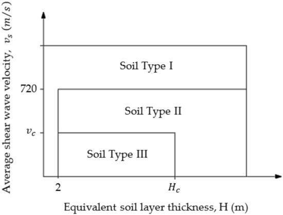
Figure 4. Soil microzoning using thickness, $H_s$, and average shear wave velocity, $v_s$, adapted with permission from Ulises Mena, Comisión Federal de Electricidad Manual de Diseño de Obras Civiles; published by Comision Federal de Electricidad (CFE), 2015 [1].

Soil type I is a rigid layer with low dynamic amplifications at the site, soil type II is a medium rigid layer that presents intermediate dynamic amplifications, and soil type III is a soft layer with high dynamic amplifications.

With the location of the seismic zone related to Figure 2 and the soil type assignment according to Figure 4, the site factor, $F_{sit}$, and the response factor, $F_{res}$, can be selected using the values shown in Table 6, where the reference spectrum (ER) and the spectral acceleration in the rock layer, $a_{0r}$, are provided by PRODISIS.

Table 6. $F_{sit}$ and $F_{res}$ factors for dynamic amplification factors at the site, reproduced with permission from Ulises Mena, Comisión Federal de Electricidad Manual de Diseño de Obras Civiles; published by Comision Federal de Electricidad (CFE), 2015 [1].

Zone	Soil Type I 1	Soil Type II	Soil Type III
A	$F_{sit}=1.0$ $F_{res}=PRODISIS$	$F_{sit}=2.6$ $F_{res}=3.8$	$F_{sit}=3.0$ $F_{res}=4.2$
B	$F_{sit}=1.0$ $F_{res}=PRODISIS$	$F_{sit}=2.6-0.2\left(\frac{a_{0r}-50}{50}\right)$ $F_{res}=3.8-0.2\left(\frac{a_{0r}-50}{50}\right)$	$F_{sit}=3.0-0.3\left(\frac{a_{0r}-50}{50}\right)$ $F_{res}=4.2-0.3\left(\frac{a_{0r}-50}{50}\right)$
C	$F_{sit}=1.0$ $F_{res}=PRODISIS$	$F_{sit}=2.4-0.3\left(\frac{a_{0r}-100}{100}\right)$ $F_{res}=3.6-0.2\left(\frac{a_{0r}-100}{100}\right)$	$F_{sit}=2.7-0.4\left(\frac{a_{0r}-100}{100}\right)$ $F_{res}=3.9-0.3\left(\frac{a_{0r}-100}{100}\right)$
D	$F_{sit}=1.0$ $F_{res}=PRODISIS$	$F_{sit}=2.1-0.5\left(\frac{a_{0r}-200}{290}\right)$ $F_{res}=3.4-0.5\left(\frac{a_{0r}-200}{290}\right)$	$F_{sit}=2.3-0.6\left(\frac{a_{0r}-200}{290}\right)$ $F_{res}=3.6-0.6\left(\frac{a_{0r}-200}{290}\right)$

¹ The response factor, $F_{res}$, for soil type I soil requires the geographic location using the seismic hazard map. Therefore, PRODISIS is required to obtain the value [4].

With the seismic zone and soil dynamic factors available, the seismic elastic design spectrum can be obtained. First, it is required to obtain the maximum accelerations, $a_0$ and $c$, by applying the following equations:

$$a_0=F_{sit}{a}_{0r}$$

(11)

$$c=F_{res}{a}_0$$

(12)

where $a_0$ is the maximum acceleration on the ground and $c$ is the maximum spectral acceleration. Due to the empirical origin of the dynamic amplification factors shown in Table 6, a few restrictions related to the spectral accelerations values are added to avoid any oversizing result, using the limits shown in Table 7.

Table 7. Limits for the spectral accelerations $a_0$ and $c$, reproduced with permission from Ulises Mena, Comisión Federal de Electricidad Manual de Diseño de Obras Civiles; published by Comision Federal de Electricidad (CFE), 2015 [1].

Acceleration	Soil Type I	Soil Type II	Soil Type III
$a_0 \left(\mathrm{cm}/{\mathrm{s}}^2\right)$	$32\le a_0\le 490$	$80\le a_0\le 690$	$94\le a_0\le 752$
$c \left(\mathrm{cm}/{\mathrm{s}}^2\right)$	$80\le c\le 1225$	$320\le c\le 2000$	$390\le c\le 2256$

The seismic elastic design spectrum is obtained with the following equations:

$$S_a\frac{\mathrm{cm}}{{\mathrm{s}}^2}=\left\{\begin{array}{ll}{a}_0+\left(c\beta -a_0\right)\frac{T_e}{T_a}& for T_e<T_a\\ c\beta & for T_a\le T_e<T_b\\ c\beta {\left(\frac{T_b}{T_e}\right)}^r& for T_b\le T_e<T_c\\ c\beta {\left(\frac{T_b}{T_e}\right)}^r{p}_c{\left(\frac{T_c}{T_e}\right)}^2& for T_e\ge T_c\end{array}\right.$$

(13)

where $S_a$ is the spectral acceleration, $\beta$ is the structural damping factor, $r$ is a spectral decay parameter, $T$ is the vibration period of the structure, and $T_a$, $T_b$, and $T_c$ are the limits of the spectral acceleration graph. The results are shown in Figure 5.

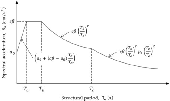
Figure 5. Seismic elastic design spectrum for structures of importance B1 and A2.

The damping factor $\beta$ is obtained with the following equation:

$$\beta =\left\{\begin{array}{cc}{\left(\frac{0.05}{{\xi }_e}\right)}^{0.45}& for T_e<T_c\\ {\left(\frac{0.05}{{\xi }_e}\right)}^{0.45\left(\frac{T_c}{T_e}\right)}& for T_e\ge T_c\end{array}\right.$$

(14)

where ${\xi }_e$ is the structural damping ratio. According to Equation (14), if ${\xi }_e=0.05$ is used, then the calculated damping factor is $\beta =1$, proving that the seismic elastic design spectrum has a default damping radio value of 5%. The $p_c$ factor is obtained with the following equation:

$$p_c=k+\left(1-k\right){\left(\frac{T_c}{T_e}\right)}^2$$

(15)

where $k$ is a spectral decay parameter for acceleration values after period $T_c$. The parameters $T_a$, $T_b$, $T_c$, $k$, and $r$ in previous equations are obtained by using the values shown in Table 8, according to the seismic zone and the soil type.

Table 8. Values of periods and exponents for the elastic design spectrum, reproduced with permission from Ulises Mena, Comisión Federal de Electricidad Manual de Diseño de Obras Civiles; published by Comision Federal de Electricidad (CFE), 2015 [1].

Zone	Soil Type	${\mathit{T}}_{\mathit{a}} \left(\mathit{s}\right)$	${\mathit{T}}_{\mathit{b}} \left(\mathit{s}\right)$	${\mathit{T}}_{\mathit{c}} \left(\mathit{s}\right)$	$\mathit{k}$	$\mathit{r}$
A	I	0.1	0.6	2.0	1.5	0.5
	II	0.2	1.4	2.0	1.0	2/3
	III	0.3	2.0	2.0	0.5	1.0
B	I	0.1	0.6	2.0	1.5	0.5
	II	0.2	1.4	2.0	1.0	2/3
	III	0.3	2.0	2.0	0.5	1.0
C	I	0.1	0.6	2.0	1.5	0.5
	II	0.2	1.4	2.0	1.0	2/3
	III	0.2	2.0	2.0	0.5	1.0
D	I	0.1	0.6	2.0	1.5	0.5
	II	0.1	1.4	2.0	1.0	2/3
	III	0.1	2.0	2.0	0.5	1.0

The seismic elastic design spectrum using the regional spectrum procedure can be modified by applying different return periods, $T_r$, and structural damping ratios, ${\xi }_e$. PRODISIS allows us to apply a specific return period, $T_r$, providing the return period reference spectrum EPR, with values used as initial inputs to apply on the procedure described instead of the reference spectrum ER inputs.

To obtain the seismic elastic design spectrum with vertical load, the spectral acceleration values are obtained using the following equation:

$$S_{av}=\left\{\begin{array}{ll}1.4 F_d{S}_a& for T_v<0.05 \mathrm{s}\\ 1.4 F_d{S}_a{\left(\frac{0.05}{T_v}\right)}^{2/3}& for T_v\ge 0.05 \mathrm{s}\end{array}\right.$$

(16)

where $S_{av}$ is the vertical spectral acceleration, $S_a$ is the horizontal spectral acceleration previously calculated, $F_d$ is the distance factor obtained as $a_{0r}/200$ with a value not greater than 1.0, $a_{0r}$ is the maximum acceleration in the rock layer of the reference spectrum ER or the return period reference spectrum EPR, and $T_v$ is the vertical vibration period of the structure.

Finally, all the spectral acceleration values, $S_a$ and $S_{av}$, must be multiplied by the structural importance factor, $F_{IE}$, previously determined in Table 3.

3.4. Site-Specific Spectrum According to MDOC Sismo CFE 2015

According to Table 3, the structures of importance A1 and A+ are related to buildings intended for the power generation industry, whose failure due to seismic events could have major negative consequences. Therefore, the spectral acceleration values require an accurate result, obtained by applying the site-specific spectrum procedure. The steps are extensive compared with the regional spectrum procedure and need different support tools, including specialized software and numerical methods. The steps for the site-specific spectrum procedure are given below.

Step 1: Obtain the reference spectrum ER or EPR in the rock layer and perform at least five synthetic accelerograms adjusted to the target spectrum.

PRODISIS requires the geographic coordinates to locate the site and obtain the reference spectrum ER or the return period reference spectrum EPR in the rock layer. Figure 3 presents the ER spectrum related to the city of Puebla, showing an optimal return period of $T_r=408 \mathrm{years}$ and its spectral acceleration graph in blue. Additionally, the EPR spectrum is shown for a provided return period of $T_r=975 \mathrm{years}$ with a spectral acceleration graph in green.

Moreover, PRODISIS has a specific section related to synthetic accelerogram calculations, where simulations are performed by applying an assigned target spectrum, either the reference spectrum ER or the return period reference spectrum EPR, with the values previously obtained. The software performs a numerical process to obtain different accelerogram simulations, compatible with the seismic spectrum input used [4].

At least five synthetic accelerogram simulations should be performed, including a compatibility check, by performing a comparison between the response spectrum of each simulation and the target spectrum used, showing a match between the results. Figure 6 gives examples of 10 synthetic accelerograms using the reference spectrum ER related to the city of Puebla, as shown previously in Figure 3.

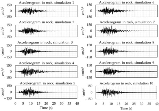
Figure 6. Synthetic accelerograms based on the reference spectrum ER in Puebla, Mexico.

There are other programs such as SeismoArtif, developed by Seismosoft Earthquake Engineering Software Solutions [5], that can be used to perform simulations of synthetic accelerograms using any target spectrum as initial input, substituting for the process performed by PRODISIS. Any number of synthetic accelerogram results can be used; the only restriction is the need to perform a compatibility check by matching the values between the response spectrum of each simulation with the target spectrum.

For each of the synthetic accelerograms in Figure 6, the response spectra are obtained and compared with the reference spectrum ER to ensure the compatibility check. This comparison can be performed within PRODISIS or SeismoArtif, providing graph results as shown in Figure 7, where the thin black lines represent the response spectrum of each synthetic accelerogram, the blue line represents the mean average of the response spectra, and the red line represents the target spectrum used. The simulation process requires the Fourier transform and wavelets methods [4,5].

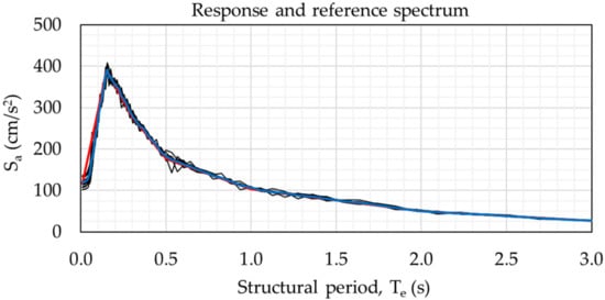
Figure 7. Response and reference spectra comparison for the city of Puebla, Mexico.

Step 2: Use the soil layers data from the site to perform the transfer function and obtain the dynamic amplification of the ground.

To perform a dynamic analysis of the soil, data on the physical properties of each layer $i$ in the site are required, focused on the thickness $h_i$, the volumetric weight ${\rho }_i$, the shear wave velocity $v_{si}$, the damping ratio ${\xi }_i$, and the total depth $H_s$. The goal is to obtain the dynamic amplification of the seismic waves at the site from the rock layer to the surface layer, according to the different frequencies. Figure 8 shows the seismic wave path from the fault to the site of interest, where the surface layer tends to amplify the seismic wave amplitudes [6].

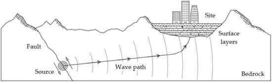
Figure 8. Path of vibrational waves from the seismic source to the surface layers.

A first approximation to study the dynamic behavior of the surface soil and the frequencies is made by applying a 1D model and taking as inputs the rock layer at the base and the thickness of each surface layer where the seismic waves can travel. The formulation used for 1D models considers the harmonic motion, where their amplitude is measured on the free surface. Figure 9 shows a scheme of wave propagation in the soil layer with thickness H, applying the functions $A{e}^{i\left(\omega t+kz\right)}$ and $B{e}^{i\left(\omega t-kz\right)}$, which are related to the wave movement in the z-axis direction.

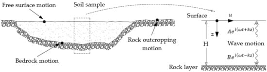
Figure 9. 1D model for the dynamic analysis between the rock and surface layers.

The functions shown in Figure 9 have different variables that define the equations of motion, where $\omega$ is the circular frequency of the ground, k is the wave number expressed as $k=\omega /v_s$, A and B are the wave amplitudes in each direction, $z$ is the height measured from the free surface layer, and $t$ is the time.

Considering the thickness of the surface soil as an equivalent layer, with damping and elastic rock at the base, the 1D model is modified according to the variables shown in Figure 10, where $H$ is the equivalent layer thickness, the subscript $s$ refers to the equivalent soil layer, and the subscript $r$ refers to the rock layer at the base. Thus, the transfer function $F_1\left(\omega \right)$ is defined as follows [6]:

$$F_1\left(\omega \right)=\frac{1}{cos\left(\frac{\omega H}{v_{ss}^{*}}\right)+i{\alpha }_z^{*}sin\left(\frac{\omega H}{v_{ss}^{*}}\right)}$$

(17)

where $v_{ss}^{*}$ is the complex wave velocity in the soil layer, defined as $v_{ss}^{*}=v_{ss}\left(1-i\xi \right)$; ${\alpha }_z^{*}$ is the complex impedances ratio, defined as ${\alpha }_z^{*}={\rho }_s{v}_{ss}^{*}/{\rho }_r{v}_{sr}^{*}$; ${\rho }_s$ is the volumetric weight of the soil layer; ${\rho }_r$ is the volumetric weight of the rock layer; and $v_{sr}^{*}$ is the complex wave velocity in the rock layer, defined as $v_{sr}^{*}=v_{sr}\left(1-i\xi \right)$.

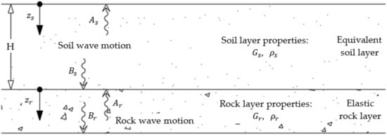
Figure 10. 1D model related to the transfer function $F_1\left(\omega \right)$ for an equivalent layer.

Now, instead of a single layer with equivalent thickness, it is convenient to consider multiple layers as damped soil over the elastic rock, modifying the 1D model according to Figure 11 to improve the results. Therefore, the transfer function, $F_2\left(\omega \right)$, related to the motion, $u\left(z,t\right)$, at layer $m$, is expressed according to the following equations:

$$u\left(z,t\right)=A{e}^{i\left(\omega t+k^{*}z\right)}+B{e}^{i\left(\omega t-k^{*}z\right)}$$

(18)

$$F_2\left(\omega \right)=\frac{\left|u_i\right|}{\left|u_j\right|}$$

(19)

where $k^{*}$ is the complex wave value, defined as $k^{*}=k\left(1-i\xi \right)$ and the subscripts $i$ and $j$ are related to the layer number.

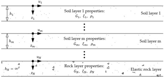
Figure 11. 1D model and the transfer function $F_2\left(\omega \right)$ for a layered soil.

The amplitude is obtained with the absolute value of the transfer function represented as $\left|F\left(\omega \right)\right|$. The described equations are applicable for a single-degree-of-freedom (SDF) system to perform a linear analysis. Now, with an iterative process, the equations can be used to perform a nonlinear analysis.

There are programs available that can numerically obtain the soil transfer functions $F\left(\omega \right)$ using 1D models, including multiple layers methods with the possibility to perform a linear or non-linear analysis. Some examples are DeepSoil, developed by the University of Illinois in Urbana, IL, USA [7], or ProShake, developed by EduPro Civil Systems Inc. in Sammamish, WA, USA [8], where the interface allows us to assign the soil layer properties using the variables shown in Figure 11 and the program calculates the transfer function, $F\left(\omega \right)$, displaying the results with a $\left|F\left(\omega \right)\right|$ vs. frequency (Hz) graph.

Figure 12 shows the transfer function $\left|F\left(\omega \right)\right|$ graph and its amplitudes for a layered soil, where the inputs are provided by MDOC Sismo CFE 2015 in its design aids section [9], showing the total thickness $H_s=30 \mathrm{m}$, layers with thickness $h_m=1 \mathrm{m}$, layer volumetric weight ${\rho }_m$ between $1420 \mathrm{and} 1800 \mathrm{kg}/{\mathrm{m}}^3$, shear wave velocities $v_m$ between $170 \mathrm{and} 340 \mathrm{m}/\mathrm{s}$, damping ratio ${\xi }_m=0.05$, rock volumetric weight ${\rho }_r=2000 \mathrm{kg}/{\mathrm{m}}^3$, and shear wave velocity in the rock layer $v_r=720 \mathrm{m}/\mathrm{s}$.

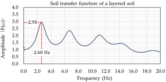
Figure 12. Transfer function graph $\left|F\left(\omega \right)\right|$ and amplitudes for a layered soil.

In Figure 12, multiple amplitudes are represented by peaks at different frequencies; the maximum value occurs in the first peak with a frequency of $f=2.6 \mathrm{Hz}$ and an amplitude of $\left|F\left(\omega \right)\right|=2.95$.

The soil can be classified into type I, II, or III according to Figure 4 and Table 5, by applying the fundamental period or the layered soil obtained with the first peak of the graph. Therefore, the inputs required are $T_s=1/f=1/2.6 \mathrm{Hz}=0.384 \mathrm{s}$, $H_s=30 \mathrm{m}$, and $v_s=4H_s/T_s=\left(4\right)\left(30 \mathrm{m}\right)/0.384 \mathrm{s}=313\mathrm{m}/\mathrm{s}$. Finally, the soil microzoning graph can be used, showing a type III soil as a result according to the values obtained from Figure 12.

For structures of the A+ subgroup, any 1D model may be insufficient to obtain the dynamic behavior of the layered soil due to the simplicity of the mathematical procedure because all wave directions must be considered and not only the vertical component. Therefore, detailed soil layer and topography data are required to create a 3D model and perform an improved dynamic analysis, using a finite element technique or similar numerical methods.

Step 3: Amplification of the synthetic accelerogram amplitudes using the previously calculated ground transfer function $F\left(\omega \right)$.

Once the synthetic accelerograms in the rock layer of step 1 and the transfer function $F\left(\omega \right)$ of step 2 are available, the amplification of the synthetic accelerograms can be obtained on the free surface of the site. To perform this step, the following equation is applied:

$$A_s\left(\omega \right)=A_r\left(\omega \right)\times F\left(\omega \right)$$

(20)

where $A_s\left(\omega \right)$ is the soil motion on the free surface of the layer as a function of the angular frequency, obtained according to the mathematical convolution process between the functions $A_r\left(\omega \right)$ and $F\left(\omega \right)$. To apply Equation (20), the accelerograms as a function of time, previously obtained via step 1, must be modified as a function of their angular frequencies, $A_r\left(\omega \right)$. To perform this step, a Fourier transform technique must be applied on each of the synthetic accelerograms previously obtained in step 1.

Once the acceleration on the free surface of the soil $A_s\left(\omega \right)$ is available, an inverse Fourier transform must be performed to modify the acceleration, now as a function of time. DeepSoil [7] and ProShake [8] can perform this mathematical process, displaying as a result each of the accelerograms modified by the transfer function.

Figure 13 shows the synthetic accelerograms modified by the Fourier transform technique according to the example presented by applying the convolution process between the functions $A_r\left(\omega \right)$ and $F\left(\omega \right)$. The maximum acceleration value of each simulation is near $200 \mathrm{cm}/{\mathrm{s}}^2$, while the accelerograms shown in Figure 6 are near $100 \mathrm{cm}/{\mathrm{s}}^2$, showing the dynamic amplification of the amplitudes due to the difference in stiffness between the surface soil and the rock layer. This phenomenon is known as site-specific conditions.

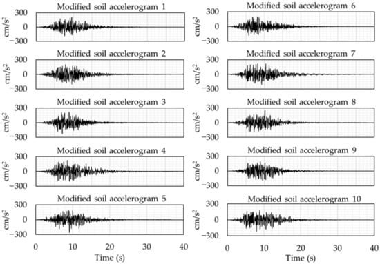
Figure 13. Synthetic accelerograms modified by the soil transfer function.

Step 4: Obtain the response spectrum geometric mean using all modified accelerogram and define periods, $T_a$ and $T_b$.

Once the modified accelerogram simulations obtained from step 3 are available, the next step is to obtain the response spectrum with a structural damping ratio ${\xi }_e=0.05$. The common methods used for this process are Newmark, Nigan–Jennings, Duhamel integral, or Fourier transform [10]. With the response spectra available, the geometric mean of all spectral acceleration values can be obtained. DeepSoil [7] and ProShake [8] can perform this numerical process, showing the result as a response spectra graph of each accelerogram including the geometric mean.

Figure 14 shows the response spectra graph of the modified accelerograms for structural periods between 0.0 and 3.0 s. The results of each simulation are represented by thin black lines and the geometric mean values by a red line.

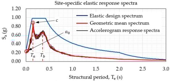
Figure 14. Graph of site-specific seismic elastic response spectra for Puebla, Mexico.

The maximum values are defined according to the geometric mean response spectrum graph shown in Figure 14 (represented in red), where the structural periods of the peak acceleration are $T_a=0.154 \mathrm{s}$ and $T_b=0.368 \mathrm{s}$. Thus, the maximum spectral acceleration coefficient values $a_0$ and $c$ correspond to $a_0=0.226 \mathrm{g}=222\mathrm{cm}/{\mathrm{s}}^2$ and $c=0.854 \mathrm{g}=838\mathrm{cm}/{\mathrm{s}}^2$.

Since the soil properties data obtained previously in step 2 can have different uncertainties, all spectral accelerations and the space between $T_a$ and $T_b$ should be increased to consider these variations, with a minimum value of 15%. Therefore, the previous variables are modified as $T_a=\left(0.85\right)\left(0.154 \mathrm{s}\right)=0.131 \mathrm{s}$, $T_b=\left(1.15\right)\left(0.368 \mathrm{s}\right)=0.423 \mathrm{s}$, $a_0=\left(1.15\right)\left(0.226 \mathrm{g}\right)=0.260 \mathrm{g}=255 \mathrm{cm}/{\mathrm{s}}^2$, and $c=\left(1.15\right)\left(0.854 \mathrm{g}\right)=0.982 \mathrm{g}=963 \mathrm{cm}/{\mathrm{s}}^2$. If an accurate precision is required, the Monte Carlo simulation technique should be performed, using the values $v_s$, ${\rho }_s$, and ${\xi }_s$ as random variables with a log-normal distribution process [9].

Step 5: Obtain the site-specific elastic design spectrum.

With the values of $a_0$, $c$, $T_a$, and $T_b$ available from step 4 and the soil type III classification from step 2, the seismic elastic design spectrum can be obtained by applying Equation (13). Figure 14 shows the results of the site-specific elastic design spectrum with a blue line.

Finally, all the spectral acceleration values, $S_a$, must be multiplied by the structural importance factor, $F_{IE}$, previously determined in Table 3.

3.5. Deterministic Spectrum According to MDOC Sismo CFE 2015

A deterministic spectrum implies a procedure to obtain the spectral accelerations as a function of a specific earthquake event, particularly of high magnitude with a shorter distance between the seismic source and the specific site. Therefore, we need the seismic records data near the site of interest to identify the appropriate seismic events and perform the analysis.

The initial inputs required to perform a deterministic spectrum are the magnitude of the earthquake, $M$, the focal length, $R$, the fault type related to the seismic event, and the distance from the hypocenters to the surface. The general analysis process is explained in MDOC Sismo CFE 2015 in its comments section [11].

The deterministic method suggests the application of the local seismicity with an appropriate attenuation of the seismic waves, by using the ground motion prediction equations (GMPE), to obtain the spectral acceleration, $S_a$, at the site of interest.

Local seismicity shows the recurrence of earthquakes according to the magnitudes registered at a particular site. The recurrence is measured with the exceedance rate $\lambda \left(M\right)$ and can be obtained by applying the modified Gutenberg–Richter relationship [12] for most seismic sources in Mexico and the characteristic seismic model [13], which works adequately for the subduction fault zone located between the Cocos and North American plates in southern Mexico. The parameters for both models are mapped for different seismic-generator zones across the country and can be found in the MDOC Sismo CFE 2015 in its comments section [11].

The ground motion prediction equations (GMPE) are models developed for seismic zones with a particular geological fault type, considering a decrease in the amplitudes of the seismic waves by getting away from the epicenter. For Mexico, three types of models are used, depending on the fault type and the hypocenter’s depth. The model of Abrahamson and Silva [14] is applied to shallow earthquakes, while the model of Zhao et al. [15] is applied to earthquakes of intermediate depth, and the model of Arroyo et al. [16] is related to interplate earthquakes according to the subduction fault. These models can be modified according to data on recent earthquakes.

Once the local seismicity has been assessed for an earthquake of magnitude, $M$, an appropriate GMPE model, and a focal length, $R$, the maximum spectral acceleration, $A_m$, can be obtained deterministically. However, there are uncertainties in the magnitude, $M$, and the focal length, $R$, that affect the spectral acceleration, $S_a$. Therefore, a log-normal distribution must be applied due to the nature of earthquakes, according to the following equation:

$$S_a=A_m\left(M,R\right)e^{\epsilon {\sigma }_{lnA}}$$

(21)

where $A_m\left(M,R\right)$ is the mean spectral acceleration for an earthquake of magnitude, M, and focal length, R, with an appropriate GMPE model, ${\sigma }_{lnA}$ is the standard deviation, and $\epsilon$ is the percentile used, with a value of $\epsilon =1$ for an 84% percentile according to the log-normal distribution.

4. Seismic Response Spectra in the USA

According to ASCE/SEI 7-16 [2], U.S. seismic hazard maps are required as initial input to obtain the seismic elastic design spectrum, with their acceleration values in terms of gravity, $\mathrm{g}$, and related to structural periods of 0.2 and 1.0 s.

Figure 15 shows the seismic hazard levels for the USA, developed by the U.S. Geological Survey (USGS) in 2018: high-seismicity zones are represented in red and low-seismicity zones in gray. The western zone has high levels of seismic hazard due to the limits between the Pacific and North American plates together with the Juan de Fuca plate. In addition, there is an intraplate fault located in the central–east zone showing high levels of seismicity [17].

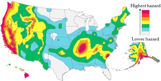
Figure 15. Seismic hazard map for the USA according to the USGS [17].

The seismic hazard maps developed for the USA consider the risk-targeted maximum considered earthquake, $MC{E}_R$, with an exceedance probability of 1% in 50 years, or a return period, $T_r=4975 \mathrm{years}$, offering the spectral acceleration values in the rock layer for different structural periods.

The code uses the spectral acceleration parameters $S_S$ and $S_1$ as inputs, which are obtained directly from the seismic hazard maps. The value of $S_S$ is related to the spectral acceleration in rock layer for a short structural period of $T=0.2 \mathrm{s}$, representing the peak in the graph of spectral accelerations; the value of $S_1$ is related to a structural period of $T=1.0 \mathrm{s}$, representing the descending part of the graph. Both parameters use a damping ratio of ${\xi }_e=0.05$.

The USGS offers the seismic hazard maps on its website, where the interface requests the geographic coordinates or the city and the interface show the spectral acceleration values related to a $MC{E}_R$ [18].

4.1. Initial Inputs for the Elastic Design Spectrum According to ASCE/SEI 7-16

To obtain the seismic elastic design spectrum, we need to have the importance of the structure, the spectral accelerations parameters, $S_S$ and $S_1$, according to the seismic hazard map related to an earthquake, $MC{E}_R$, and the soil physical properties, used to perform the dynamic amplifications due to the site effects.

The risk category classification applied to each structure depends of the use of the structure, where a probability of failure by $MC{E}_R$ and a structural importance factor, $I_e$, are assigned [2].

Risk category I is related to common structures with a probability of failure by $MC{E}_R$ of 10% in 50 years and an importance factor of 1.0; risk category III is focused on the energy sector, such as hydroelectric and nuclear plants, where their failure can have negative economic impacts and lead to environmental catastrophes, using a probability of failure by $MC{E}_R$ of 5% in 50 years and an importance factor of 1.25; risk category IV is related to the same structures of category III with a very high risk, using a probability of failure of 2.5% and an importance factor of 1.5; finally, risk category II is related to all other structures except of the previous risk categories, using the same probability of failure and importance factor assigned in category I.

To consider the dynamic amplification of the ground due to the site effects, a physical soil study must be performed on the field using available methods, such as cross hole or the equivalent, to obtain the dynamic properties of the layers and assign a site class.

As in Figure 11, previously shown as an example, the physical properties of each layer, $i$, are required, such as the thickness, $d_i$, the shear wave velocity, $v_{si}$, the volumetric weights, ${\rho }_i$, the damping ratio, ${\xi }_i$, the number of blows of the standard penetration resistance, $N_i$, and the shear stress, $s_{ui}$. A minimum soil thickness $H=30 \mathrm{m}$ is required to obtain the dynamic properties [2].

According to ASCE/SEI 7-16, the soil can be classified from site class A to F, where class A is very stiff rock and class F very soft soil. The variables used to classify the soil are the average shear wave velocity ${\overline{v}}_s$, the average standard penetration resistance $\overline{N}$ and the average undrained shear stress ${\overline{s}}_u$.

Site class A and B are related to rock soils where ${\overline{v}}_s$ is used; site class C and D are related to dense and stiff soils, using one of the different values of ${\overline{v}}_s$, $\overline{N}$ and ${\overline{s}}_u$; site class E and F are related to soft soils where different mechanical and dynamic properties are required. The values of ${\overline{v}}_s$, $\overline{N}$ and ${\overline{s}}_u$ required to classify the site are located in chapter 20 of ASCE/SEI 7-16 [2].

Therefore, for a layered soil, as shown in Figure 11, the average shear wave velocity, $v_s$, is obtained according to the following equation:

$${\overline{v}}_s=\frac{{{\displaystyle \sum }}_{i=1}^n{d}_i}{{{\displaystyle \sum }}_{i=1}^n\frac{d_i}{v_{si}}}$$

(22)

where subscript $i$ refers to a layer, $d_i$ is the thickness of layer $i$, $v_{si}$ is the shear wave velocity of layer $i$, and $n$ is the number of layers. To obtain the average standard penetration resistance for cohesionless soils, $\overline{N}$, the following equation is used:

$$\overline{N}=\frac{{{\displaystyle \sum }}_{i=1}^n{d}_i}{{{\displaystyle \sum }}_{i=1}^n\frac{d_i}{N_i}}$$

(23)

where $N_i$ is the standard penetration resistance for layer $i$; the values $N_i$ and $d_i$ are related to cohesionless soil, cohesive soil, and rock layers. Now, exclusively for cohesionless soils, the value of ${\overline{N}}_{ch}$ is obtained with the following equation:

$${\overline{N}}_{ch}=\frac{d_s}{{{\displaystyle \sum }}_{i=1}^m\frac{d_i}{N_i}}$$

(24)

where $m$ is the number of cohesionless layers; the values of $N_i$ and $d_i$ are related exclusively to cohesionless soil. The value $d_s$ is obtained with the following equation:

$${{\displaystyle \sum }}_{i=1}^m{d}_i=d_s$$

(25)

where $d_s$ is the total thickness of the cohesionless soil. The average undrained shear stress ${\overline{s}}_u$ is determined by the following equation:

$${\overline{s}}_u=\frac{d_c}{{{\displaystyle \sum }}_{i=1}^k\frac{d_i}{s_{ui}}}$$

(26)

where $s_{ui}$ is the shear stress in layer $i$ and $d_c$ is the total thickness of cohesive soil layers, whose value is obtained via the following equation:

$${{\displaystyle \sum }}_{i=1}^k{d}_i=d_c$$

(27)

where $k$ is the number of cohesive soil layers and $d_i$ is the thickness of cohesive soil layer $i$.

4.2. Regional Spectrum According to ASCE/SEI 7-16

To obtain the seismic elastic design spectrum, we must know the location of the site and the physical properties of the soil as initial inputs. With the geographical location of the site on the U.S. seismic hazard map, it is possible to obtain the spectral accelerations in rock for a risk-targeted maximum considered earthquake, $MC{E}_R$, using the parameter $S_s$ for a short structural period of $T_e=0.2 \mathrm{s}$ and the parameter $S_1$ for periods of $T_e=1.0 \mathrm{s}$.

With the soil properties available, the site can be classified between classes A and F. If the soil properties are not available, ASCE/SEI 7-16 recommends applying class D, unless a study is required due to the nature of the structure or the soil physical conditions can be classified as site class E or F [2].

First, the spectral accelerations parameters, $S_S$ and $S_1$, related to an earthquake, $MC{E}_R$, need to be modified by using the site class coefficients to obtain the modified response spectral acceleration parameter, $S_{MS}$, for short structural periods of 0.2 s and $S_{M1}$ for periods of 1.0 s, according to the following equations:

$$S_{MS}=F_a{S}_S$$

(28)

$$S_{M1}=F_v{S}_1$$

(29)

where $S_S$ and $S_1$ are the spectral response acceleration parameters obtained from the $MC{E}_R$ at short and long periods, $F_a$ is the site coefficient for short periods, and $F_v$ is the site coefficient for long periods. The coefficients $F_a$ and $F_v$ are obtained using different tables provided in chapter 11 of ASCE/SEI 7-16, depending on the site class and the mapped spectral acceleration parameters [2].

The design spectral acceleration parameters, $S_{DS}$ for short periods and $S_{D1}$ for long periods, are determined via the following equations:

$$S_{DS}=\frac{2}{3}{S}_{MS}$$

(30)

$$S_{D1}=\frac{2}{3}{S}_{M1}$$

(31)

where the $S_{MS}$ and $S_{M1}$ values, multiplied by the factor of 2/3, indirectly modify the $MC{E}_R$ from a return period of $T_r=4975 \mathrm{years}$ (with a 1% probability of failure in 50 years) to an $MCE$ with a return period of $T_r=475 \mathrm{years}$ (with a 10% probability of failure in 50 years).

To obtain the seismic elastic design spectrum with a 5% of structural damping ratio, the following equations are used:

$$S_a\left(g\right)=\left\{\begin{array}{l}\begin{array}{cc}{S}_{DS}\left(0.4+0.6\frac{T}{T_0}\right) & 0<T<T_0\end{array}\\ \begin{array}{cc} S_{DS} & T_0\le T\le T_S\\ \frac{S_{D1}}{T} & T_S<T\le T_L\\ \frac{S_{D1}{T}_L}{T^2} & T>T_L\end{array}\end{array}\right.$$

(32)

Figure 16 shows the spectral acceleration according to the previous equations with the location of parameters $S_{DS}$ and $S_{D1}$. According to the graph, $T$ is the structural period in seconds; $T_0$ and $T_S$ are the periods used as limits between the maximum acceleration value, obtained with the following equations:

$$T_0=0.2\frac{S_{D1}}{D_{DS}}$$

(33)

$$T_S=\frac{S_{D1}}{S_{DS}}$$

(34)

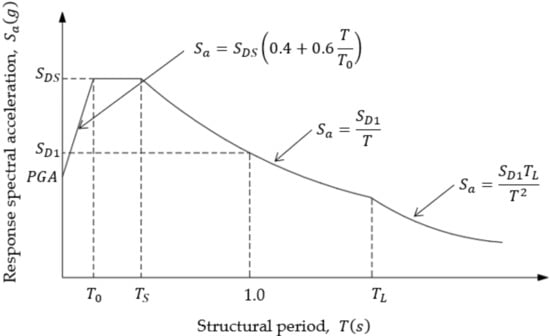
Figure 16. Seismic elastic design spectrum for site class A to D.

$T_L$ is the long transition period, which is assigned depending on the geographical location of the site. Since $T_L\ge 4 \mathrm{s}$, its application is related to structures with seismic isolators or damping systems, where the calculated structural periods usually have high values.

PGA is the peak ground acceleration value at period $T=0 \mathrm{s}$. The seismic elastic design spectrum obtained with the previous equations corresponds to a $MCE$ with a return period of $T_r=475 \mathrm{years}$. If a design spectrum for a $MC{E}_R$ with a return period of $T_r=4975 \mathrm{years}$ is required, the $S_a\left(g\right)$ values in Equation (32) must be multiplied by 1.5. Additionally, to consider the importance factor, $I_e$, all $S_a\left(g\right)$ values must be multiplied by the factor provided according to the risk category.

If a structural damping ratio value other than 5% is required, ASCE/SEI 41-17 presents the modified spectral accelerations, $S_a\left(g\right)$, by applying the provided damping value according to the following equations [19]:

$$S_a\left(g\right)=\left\{\begin{array}{c}\begin{array}{cc}{S}_{DS}\left[\left(\frac{5}{B_1}-2\right)\frac{T}{T_S}+0.4\right] & 0<T<T_0\end{array}\\ \begin{array}{cc}\frac{S_{DS}}{B_1} & T_0\le T\le T_S\\ \frac{S_{D1}}{B_{1}T} & T_S<T\le T_L\\ \frac{S_{D1}{T}_L}{B_1{T}^2} & T>T_L\end{array}\end{array}\right.$$

(35)

where $B_1$ is the effective damping coefficient, with a value of $B_1=1.0$ for an effective damping ratio of $\xi =0.05$. For calculated values of $B_1$, the following equation should be used:

$$B_1=\frac{4}{5.6-ln\left(100\xi \right)}$$

(36)

4.3. Constant Acceleration Spectrum According to ASCE/SEI 7-16

When the design of earthquake-resistant structures applies simplified methods and the dynamic properties of the soil or structure are not required, the constant acceleration spectrum procedure can be selected for a damping ratio of 5%. Using the spectral acceleration parameter for short periods, $S_S$, the following equation is applied:

$$S_a\left(g\right)=S_{DS}=\frac{2}{3}{F}_a{S}_S$$

(37)

where $S_S$ is the spectral acceleration parameter of $MC{E}_R$ for short periods and $F_a$ is the site factor for short periods, using a value of 1.0 for rock soils and 1.4 for other soil types, or the factors of chapter 11 of ASCE/SEI 7-16 for an adjusted value [2]. A rock soil is when there is a maximum thickness of 3 m between the free surface and the rock base at the site.

The constant acceleration spectrum procedure is usually applied to structures of risk category I or II, including the importance factor $I_e=1.0$, which multiplies the value of $S_{DS}$.

Finally, if a damping ratio with a value other than 5% is required, the following equation is applied:

$$S_a\left(g\right)=\frac{S_{DS}}{B_1}$$

(38)

where $B_1$ is the effective damping coefficient obtained via Equation (36).

4.4. Site-Specific Spectrum According to ASCE/SEI 7-16

For soils previously determined to be with site class E or F, it is required to obtain the seismic elastic design spectrum by taking into account the dynamic amplifications of the ground for specific sites. Additionally, a dynamic soil analysis must be performed when $S_S\ge 1.0$ for site class E, $S_1\ge 0.2$ for site classes D and E [2].

Similar to MDOC Sismo CFE 2015 code, we must follow a few steps to obtain the dynamic amplifications of the ground and apply them to a series of accelerograms in the rock layer to modify the spectral acceleration values. The process is shown below.

Step 1: Obtain the spectrum using an $MC{E}_R$ in the rock layer and simulate at least five synthetic accelerograms adjusted to the target spectrum, or select five representative accelerograms of real earthquakes.

First, the geographic site location is required to obtain the spectral acceleration parameters, $S_S$ and $S_1$, to create the seismic elastic design spectrum for an $MC{E}_R$, with the soil factors $F_a$ and $F_v$ in rock related to site class B, using the same process for the regional spectrum procedure previously described. A class A site can be used when the average shear wave velocity in the ground is ${\overline{v}}_s\ge 1524 \mathrm{m}/\mathrm{s}$ [2].

With the $MC{E}_R$ spectrum in rock available, the graph will be used as a target spectrum and at least five synthetic accelerograms should be performed, similar to step 1 of the site-specific spectrum procedure of the MDOC Sismo CFE 2015 described in Section 3.4. SeismoArtif can be used to simulate the synthetic accelerogram, reviewing whether the response spectra of each simulation are compatible with the target spectrum [5].

Alternatively, at least five real recorded earthquakes can be selected to perform an appropriate scaling process to fit the target spectrum. The selection of the accelerograms must consider the conditions of the site, such as the magnitude, the geological fault type, and the distance between the seismic event and the site location. The Pacific Earthquake Engineering Research Center, or PEER, has a database of accelerogram records on its website, with the option to select real earthquakes using a target spectrum, either defined by the user, PEER, and/or ASCE recommendations [20].

Figure 17 shows an example of a response spectral acceleration graph with a logarithmic scale, taking as a target spectrum the location of El Centro, California, and the scaling results of the selected 10 real earthquakes, including a geometric mean spectrum with a damping ratio of 5%.

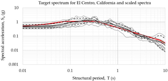
Figure 17. Example of the target spectrum for El Centro, CA, and scaled real earthquakes.

According to the previous figure, the red line represents the target spectrum, the thick black line represents the geometric mean spectrum of the real earthquakes, and the thin gray lines represent the spectra of the 10 adjusted earthquakes. A good fit between the target spectrum and the mean values can be observed between 0.1 to 10 s.

Step 2: Obtain the soil layer inputs and perform the transfer function to consider the dynamic site effects.

The inputs related to the physical properties of the soil layers and the procedure to obtain the transfer function, $F\left(\omega \right)$, are explained in step 2 previously presented in the site-specific spectrum of the MDOC Sismo CFE 2015 code in Section 3.4. Programs such as DeepSoil [7] or ProShake [8] can be used to create a 1D model of the soil layers to obtain the graph of the transfer function, $F\left(\omega \right)$, by applying linear or non-linear analysis procedures.

Step 3: Perform the amplification of the scaled synthetic and/or real accelerograms by applying the ground transfer function $F\left(\omega \right)$.

Once the graph of the soil transfer function, $F\left(\omega \right)$, is available from step 2, the accelerograms obtained in step 1 must be scaled. The process is similar to step 3, previously presented in the site-specific spectrum of MDOC Sismo CFE 2015 in Section 3.4.

The accelerograms must be modified from a time function to a frequency function, $A_r\left(\omega \right)$, by applying the Fourier transform technique, performing the mathematical convolution process between the functions $A_r\left(\omega \right)$ and $F\left(\omega \right)$, and then, applying an inverse Fourier transform to return the accelerations as a function of time. DeepSoil [7] and ProShake [8] can perform this mathematical process and obtain scaled accelerograms according to the soil dynamic properties related to the transfer function.

Step 4: Obtain the mean response spectrum for all accelerograms and define the structural periods, $T_0$ and $T_s$.

For each accelerogram previously modified with the transfer function, the response spectrum of each accelerogram and the geometric mean can be obtained. The process is similar to step 4 previously presented in Section 3.4.

Using DeepSoil [7] or ProShake [8] programs, the geometric mean response spectrum can be obtained. With the spectral graph available, it is possible to visually determine the periods and maximum spectral acceleration values, where the parameter $S_{DS}$ for short periods is located between the periods $T_0$ and $T_S$ and the parameter $S_{D1}$ is located at a period of 1.0 s. The period $T_L$ can be obtained directly from ASCE/SEI 7-16 maps [2] or USGS webpage [18].

Finally, an increase of at least 15% in $S_{DS}$ and $S_{D1}$ values must be created, including the distance between the periods $T_0$ and $T_S$, due to the uncertainties in the soil layer inputs related to the field. As an alternative procedure, a Monte Carlo simulation can be performed to obtain an adjusted amplification percentage to be applied on the previous parameters.

Step 5: Obtain the elastic design spectrum for the study site.

With the acceleration values, $S_{DS}$ and $S_{D1}$, the periods $T_0$ and $T_S$ previously obtained in step 4, and period $T_L$ from the maps provided by ASCE/SEI 7-16, the elastic design spectrum can be developed by applying Equation (32).

4.5. Deterministic Spectrum According to ASCE/SEI 7-16

For structures of risk category III or IV, the seismic elastic design spectrum based on the deterministic procedure is recommended, using the $MCE$ at the site of interest. Similar to the deterministic spectrum section shown in MDOC Sismo CFE 2015 in Section 3.5, the initial inputs required to perform the process are the magnitude of the selected earthquake, $M$, the focal length, $R$, the geological fault type, and the hypocenter depth distance.

The process involves the application of the local seismicity and appropriate ground motion prediction equations (GMPE) according to the seismic zone to perform the spectral acceleration, $S_a$, considering a log-normal distribution with 84% and a damping ratio of 5% [2].

To consider the soil dynamic effects, site classes A, B, and C require applying factors $F_a$ and $F_v$ with the values shown in chapter 11 of ASCE/SEI 7-16, according to the spectral parameter values of $S_S=1.5$ and $S_1=0.6$. For site class D, the factors $F_a=1.0$ and $F_v=2.5$ are taken. Finally, for site class E and F, the values of $F_a=1.0$ and $F_v=4.0$ are selected [2].

To obtain the seismic elastic design spectrum for an $MCE$ with a deterministic procedure, the following equation is applied:

$$S_a\left(g\right)=\frac{2}{3}{S}_{aM}$$

(39)

where $S_{aM}$ is the response spectral acceleration for a previously calculated $MCE$ with the factors $F_a$ and $F_v$ applied. Finally, the spectral acceleration values obtained with the previous equation must not be less than the limits values established in the following equation:

$$S_a\left(g\right)=\left\{\begin{array}{c}\begin{array}{cc}0.6F_a & T=0\end{array}\\ \begin{array}{cc}1.5F_a& T_0\le T\le T_S\\ \frac{0.6F_v}{T}& T_S<T\le T_L\\ \frac{0.6F_v{T}_L}{T^2}& T>T_L\end{array}\end{array}\right.$$

(40)

where $T_0=0.08F_v/F_a$ and $T_S=0.4F_v/F_a$. Figure 18 shows the shape of the spectral acceleration graph with the lower limit values according to Equation (40).

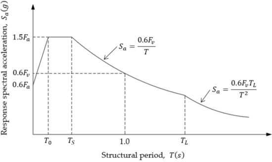
Figure 18. Lower limit of deterministic response spectrum for risk category III and IV.

5. International Seismic Response Spectra According to IBC 2018

According to IBC 2018 [3], the seismic elastic design spectrum is obtained by applying the same methodology described in ASCE/SEI 7-16, using the response spectrum in the rock layer of each country as initial inputs. The risk-targeted maximum considered Earthquake $MC{E}_R$ is taken as a reference, with a return period of $T_r=4975 \mathrm{years}$ and the parameters $S_S$ and $S_1$ for short and long structural periods. Thus, the site-specific, regional, and constant acceleration spectrum procedures use the same equations and steps described in previous sections. Therefore, each country must have the seismic hazard maps available for an $MC{E}_R$ with $T_r=4975 \mathrm{years}$.

6. Seismic Response Spectra Criteria between Codes

The previous sections described the seismic response spectra according to MDOC Sismo CFE 2015, ASCE/SEI 7-16, and IBC 2018, showing the procedure used according to the importance of the structure. Since each code has differences in the seismic inputs and soil factors, Table 9 and Table 10 show an overview of the criteria used for each code to obtain the response spectra.

Table 9. Seismic response spectra criteria and comparison between codes.

Spectrum Criteria	Inputs or Factors	MDOC Sismo CFE 2015	ASCE-SEI 7/16	IBC 2018
Constant acceleration spectrum	Seismic hazard maps source	PRODISIS	USGS website	Seismic hazard maps of each country or region
	Spectral inputs from seismic hazard maps	$a_{0r}$	$S_S$	$S_S$
	Soil factors	$F_{sit}, F_{res}$	$F_a$	$F_a$
	Software aids	PRODISIS	ASCE-SEI 7/16 website	Depends on each country or region
Regional spectrum	Seismic hazard maps source	PRODISIS	USGS website	Seismic hazard maps of the country or region
	Spectral inputs from seismic hazard maps	$a_{0r}$	$S_S, S_1$	$S_S, S_1$
	Soil inputs for site class	$T_s, H_s, v_s$	${\overline{v}}_s, \overline{N}, {\overline{s}}_u$	${\overline{v}}_s, \overline{N}, {\overline{s}}_u$
	Soil factors	$F_{sit}, F_{res}$	$F_a, F_v$	$F_a, F_v$
	Software aids	PRODISIS	ASCE-SEI 7/16 website	Depends on the country or region
Site-specific spectrum	Seismic hazard maps source	PRODISIS	USGS website, PEER website	Seismic hazard maps of the country or region
	Spectral inputs from seismic hazard maps	Spectral acceleration of the site in rock layer	Spectral acceleration in rock layer, using site class B	Spectral acceleration in rock layer, using site class B
	Accelerograms inputs	Minimum of five syntheticaccelerograms	Minimum of five synthetic accelerograms or five real earthquakes	Minimum of five synthetic accelerograms or five real earthquakes
	Soil inputs for site class	Layered soil with dynamic properties	Layered soil with dynamic properties	Layered soil with dynamic properties
	Soil factors	1D model: Soil transfer function $F\left(\omega \right)$	1D Model: soil transfer function $F\left(\omega \right)$	1D Model: soil transfer function $F\left(\omega \right)$
		3D FEM model: Related to structures of group A+
	Software aids	PRODISIS, DeepSoil, ProShake	DeepSoil, ProShake	DeepSoil, ProShake

Table 10. Deterministic seismic response spectra criteria and comparison between codes.

Spectrum Criteria	Inputs or Factors	MDOC Sismo CFE 2015	ASCE-SEI 7/16	IBC 2018
Deterministic spectrum	Seismic inputs	Seismic source, magnitude $M$, focal length $R$	Seismic source, magnitude $M$, focal length $R$	Seismic source, magnitude $M$, focal length $R$
	Spectral inputs from deterministic procedure	Spectral acceleration of the site in rock layer	Spectral acceleration in rock layer, using site class B	Spectral acceleration in rock layer, using site class B
	Accelerograms inputs	Minimum of five synthetic accelerograms	Minimum of five synthetic accelerograms or five real earthquakes	Minimum of five synthetic accelerograms or five real earthquakes
	Soil inputs for site class	Layered soil with dynamic properties	Layered soil with dynamic properties	Layered soil with dynamic properties
	Soil factors	1D model: soil transfer function $F\left(\omega \right)$	1D Model: soil transfer function $F\left(\omega \right)$	1D Model: soil transfer function $F\left(\omega \right)$
		3D FEM model: related to structures of group A+
	Software aids	PRODISIS, DeepSoil, ProShake	DeepSoil, ProShake	DeepSoil, ProShake

According to Table 9, the spectrum criteria used on each seismic code is presented, showing the minimum values required. The constant acceleration and regional spectrum criteria use a few seismic inputs, where the spectral acceleration in the rock layer does not require the entire graph of $T \mathrm{vs}. S_a$ and the site class use provides factors according to the soil type. Each seismic code has different inputs and factors we can use to assess the spectrum criteria.

According to Table 9 and Table 10, site-specific and deterministic spectrum criteria require all inputs, which means the entire spectral acceleration graph in the rock layer and the complete soil dynamic properties of the site are needed to perform an extensive mathematical process, where the calculated response spectra will show lower and more accurate spectral values compared with the constant acceleration and regional spectrum criteria. The process used for each seismic code is similar, where the main difference is the response spectra in the rock layer input.

7. Response Spectrum with ADRS Format

The seismic elastic design spectra explained previously in MDOC Sismo CFE 2015, ASCE/SEI 7-16, and IBC 2018 codes show graphs of the spectral acceleration values using a $T\mathrm{vs}.S_a$ format; these are widely used in traditional seismic engineering of structures as inputs for modal analysis methods.

However, performance-based seismic engineering requires a response spectrum with a $S_d \mathrm{vs}. S_a$ format, called acceleration displacement response spectra or ADRS format. The codes ATC-40 [21] and SEAOC 1999 [22] explain how this format is used with the static non-linear pushover analysis procedure to obtain the capacity curve graph of the buildings and the target displacement as a result.

Figure 19 shows an example of the ADRS format, representing the seismic elastic design spectra according to MDOC Sismo CFE 2015 building code, showing the spectral values of Mexicali, Mexico, with a soil type I and different damping values. According to the ADRS format, with a single graph it is possible to obtain the spectral displacements and accelerations of the structure at the same time, where the radial dotted lines represent the period $T$. The process of obtaining each radial line requires the location of a single point using the coordinates $S_d$ and $S_a$, with both values related to a specific period, $T$; one can simply draw a straight line from the origin to the point destination.

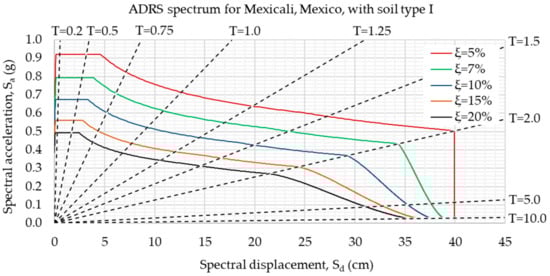
Figure 19. Example of ADRS response spectra used on several designs.

To obtain the elastic spectrum in ADRS format, acceleration values with $T \mathrm{vs}. S_a$ format are required as inputs, related to a specific damping ratio $\xi$. Then, the spectral displacements, $S_d$, can be obtained according to the following equation:

$$S_d=\frac{T^2}{4{\pi }^2}{S}_{a}g$$

(41)

where $T$ is the structural period and $S_a$ is the spectral acceleration in terms of $\mathrm{g}$. Once the spectral displacement $S_d$ values are available, the response spectrum in ADRS format can be obtained according to the $S_d \mathrm{vs}. S_a$ format.

8. Conclusions

The initial inputs required to obtain seismic elastic design spectra are the seismic hazard maps of each country or region, with the seismic intensities determined by applying deterministic and probabilistic methods according to the earthquake records of the zones. Without these maps showing the spectral values in the rock layer as available inputs, the seismic spectra cannot be determined, which affects the design of earthquake-resistant structures and procedures.

According to the Mexican, U.S., and international codes described in this review article, by obtaining the seismic elastic design spectra of common structures we can select the constant acceleration and regional spectrum criteria, offering a simple procedure without the need for specialized programs. However, these procedures apply pre-established factors related to the dynamic amplification factors of the soil, which have high and conservative values; this is a disadvantage for structures of high importance because it overestimates the spectral values, affecting the project costs.

Therefore, site-specific and deterministic spectrum criteria are applied mainly to structures of high importance, due to the extensive mathematical process required to obtain the spectral acceleration, which reduces conservatism compared with the regional spectrum. The dynamic behavior of the ground is obtained by creating a 1D model of the soil layers with the aid of specialized software, showing fewer conservative values and offering good structural safety.

If we compare the procedures described in the MDOC Sismo CFE 2015 and ASCE/SEI 7-16 codes, there are differences related to the initial inputs used to obtain the seismic response spectra, mainly in terms of the constant acceleration and regional spectrum criteria. First, the Mexican code used accelerations in the rock layer $a_{0r}$ as input, provided by PRODISIS with an optimal return period. On the other hand, the U.S. code used the spectral accelerations $S_S$ and $S_1$ related to short and long structural periods, using an $MC{E}_R$ with a return period of $T_r=4975 \mathrm{years}$. To obtain the soil class of the site, the Mexican code requires the fundamental period of the soil, $T_s$, with the values of $v_s$ and $H_s$, whereas the U.S. code required the values of ${\overline{v}}_s$, $\overline{N}$, and ${\overline{s}}_u$. Both codes used different parametric factors related to the dynamic behavior of the ground, depending on the soil class.

Now, for the site-specific spectrum criteria, the procedure is similar between the codes, using a series of steps to modify the response spectrum in the rock layer, obtained from simulations or real earthquakes with the dynamic properties of the soil according to the transfer function, $F\left(\omega \right)$. Both codes offer the option to start the procedure with the response spectra in the rock layer as an input to obtain the simulated accelerograms, according to the hazard maps.

The deterministic spectrum criteria offer the option to obtain response spectra in the rock layer for a specific earthquake, substituting the hazard maps provided by the codes. However, this procedure requires knowledge of the local seismicity, a proper GMPE selection according to the seismic zone, the magnitude of the selected earthquake, and the focal length between the source and the site. With the previous inputs available, both codes provide the option to apply a log-normal distribution process with 84% to obtain the deterministic spectral acceleration.

The procedures provided on the Mexican, U.S., and international codes to obtain the elastic design spectrum, from the constant acceleration to site-specific criteria, require an understanding of the structural project needs, where the location, use, size, and importance are required factors for proper criteria selection. A site-specific spectrum will always be less conservative compared with a constant acceleration or regional spectrum, however, the time-consuming and costly nature of this procedure for common structures makes it unaffordable. Therefore, the use of those conservative methods is justified.

Finally, the seismic elastic response spectra covered on the described codes are related to traditional seismic engineering, which uses a graph with a $T \mathrm{vs}. S_a$ format to perform the dynamic analysis of the structure according to the modal shapes. However, performance-based seismic engineering uses the same response spectra with a different format to perform the capacity curve technique, a process requiring graphs in $S_d\mathrm{vs}.S_a$ format to obtain the target displacement of the roof on the structure. Therefore, the response spectrum with $T \mathrm{vs}. S_a$ format can be modified into $S_d\mathrm{vs}.S_a$ format, making the seismic load input compatible with the performance-based method.

References

- Hernández, U.M.; Rocha, L.E.P.; Aguilera, M.D.; Alarcón, N.A. MDOC Sismo CFE 2015. Capitulo C.1.3: Diseño por Sismo, Recomendaciones. In Manual de Diseño de Obras Civiles; Comision Federal de Electricidad: Mexico City, Mexico, 2015. [Google Scholar]
- ASCE/SEI 7-16. Minimum Design Loads and Associated Criteria for Buildings and Other Structures. American Society of Civil Engineers: Reston, VA, USA, 2017. [Google Scholar]
- IBC-2018. International Building Code; International Code Council: Country Club Hills, IL, USA, 2017. [Google Scholar]
- Instituto de Investigaciones Electricas, IIE. Programa de Diseño Sismico, PRODISIS. 2015. Available online: https://www2.ineel.mx/prodisis/es/prodisis.php (accessed on 31 October 2021).
- Earthquake Engineering Software Solutions, SEiSMOSOFT. Earthquake Software for Artificial Accelerograms Generations, SeismoArtif. Available online: https://seismosoft.com/products/seismoartif/ (accessed on 2 November 2021).
- Kramer, S.L. Chapter 7: Ground Response Analysis. In Geotechnical Earthquake Engineering, 1st ed.; Prentice Hall: Hoboken, NJ, USA; pp. 254–307.
- Hashash, Y.; Musgrove, M.; Harmon, J.; Ilhan, O.; Xing, G.; Numanoglu, O.; Groholski, D.; Phillips, C.; Park, D. DEEPSOIL 7.0; User Manual: Urbana, IL, USA, 2020; Available online: http://deepsoil.cee.illinois.edu/ (accessed on 5 November 2021).
- EduPro Civil Systems, Inc. ProShake 2.0. One-Dimensional, Equivalent Linear Ground Response Analysis. Available online: http://www.proshake.com/ (accessed on 5 November 2021).
- Hernández, U.M.; Rocha, L.E.P.; Aguilera, M.D.; Alarcón, N.A. MDOC Sismo CFE 2015. Capitulo C.1.3: Diseño. In Manual de Diseño de Obras Civiles; Comision Federal de Electricidad: Mexico City, Mexico, 2015. [Google Scholar]
- Chopra, A. Dynamics of Structures, Theory and Application to Earthquake Engineering, 5th ed.; Prentice Hall: Hoboken, NJ, USA, 2017. [Google Scholar]
- Hernández, U.M.; Rocha, L.E.P.; Aguilera, M.D.; Alarcón, N.A. MDOC Sismo CFE 2015. Capitulo C.1.3: Diseño por Sismo, Comentarios. In Manual de Diseño de Obras Civiles; Comision Federal de Electricidad: Mexico City, Mexico, 2015. [Google Scholar]
- Cornell, C.A.; Vanmarcke, E.H. The Major Influences on Seismic Risk. In Proceedings of the 4th World Conference on Earthquake Engineering, Santiago, Chile, 13–18 January 1969; Volume A-1; Universidad de Chile, Facultad de Ciencias Físicas y Matemáticas: Santiago, Chile, 1969; pp. 69–83. [Google Scholar]
- Singh, S.K.; Astiz, L.; Havskov, J. Seismic Gaps and Recurrence Periods of Large Earthaquekes Along the Mexican Subduction Zone: A Reexamination. Bull. Seismol. Soc. Am. 1981, 71, 827–843. [Google Scholar] [CrossRef]
- Abrahamson, N.A.; Silva, W.J. Empirical Response Spectral Attenuation Relations for Shallow Crustal Earthquakes. Seismol. Res. Lett. 1997, 68, 1–34. [Google Scholar] [CrossRef] [Green Version]
- Zhao, J.X.; Zhang, J.; Asano, A.; Ohno, Y.; Oouchi, T.; Takahashi, T.; Ogawa, H.; Irikura, K.; Thio, H.K.; Somerville, P.G.; et al. Attenuation Relations of Strong Motion in Japan Using Site Classification Based on Predominand Period. Bull. Seismol. Soc. Am. 2006, 96, 898–913. [Google Scholar] [CrossRef]
- Arroyo, D.; García, D.; Ordaz, M.; Mora, M.A.; Singh, S.K. Strong Ground Motion Relations for Mexican Interplate Eartquakes. J. Seismol. 2010, 15, 261–294. [Google Scholar]
- U.S. Geological Survey (USGS). Earthquake Hazard Maps. Available online: https://doi.org/10.5066/F7HT2MHG (accessed on 17 November 2021).
- U.S. Geological Survey (USGS). Seismic Design Ground Motions. Available online: https://doi.org/10.5066/F7NK3C76 (accessed on 17 November 2021).
- ASCE/SEI 41-17. Seismic Evaluation and Retrofit of Existing Buildings. American Society of Civil Engineers: Reston, VA, USA, 2017.
- Pacific Earthquake Engineering Research Center (PEER). PEER Ground Motion Database. Available online: https://ngawest2.berkeley.edu/site (accessed on 20 November 2021).
- ATC-40. Seismic Evaluation and Retrofit of Concrete Buildings, Volume 1. Applied Technology Council: Redwood City, CA, USA, 1996. [Google Scholar]
- Structural Engineers Association of California. SEAOC-1999 Recommended Lateral Force Requirements and Commentary, 7th ed.; Structural Engineers Association of California: Sacramento, CA, USA, 1999. [Google Scholar]
Publisher’s Note: MDPI stays neutral with regard to jurisdictional claims in published maps and institutional affiliations. |
© 2022 by the authors. Licensee MDPI, Basel, Switzerland. This article is an open access article distributed under the terms and conditions of the Creative Commons Attribution (CC BY) license (https://creativecommons.org/licenses/by/4.0/).