Author Contributions
Conceptualization, X.M. and Z.Z.; methodology, X.M. and Z.Z.; software, D.W. and Z.Z.; validation, Y.L. and H.Y.; formal analysis, H.Y.; investigation, Y.L.; resources, Y.L.; data curation, Z.Z.; writing—original draft preparation, X.M. and Z.Z.; writing—review and editing, X.M. and Z.Z.; visualization, Z.Z.; supervision, Y.L.; project administration, Y.L.; funding acquisition, Y.L. All authors have read and agreed to the published version of the manuscript.
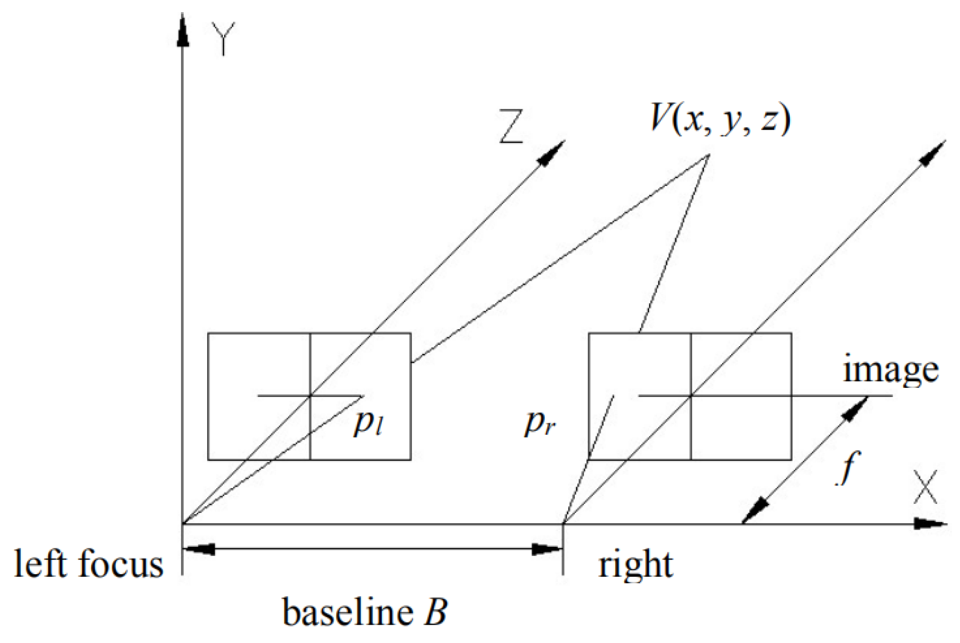
Figure 1.
Binocular vision camera model converts binocular vision into a coordinate system.
Figure 1.
Binocular vision camera model converts binocular vision into a coordinate system.
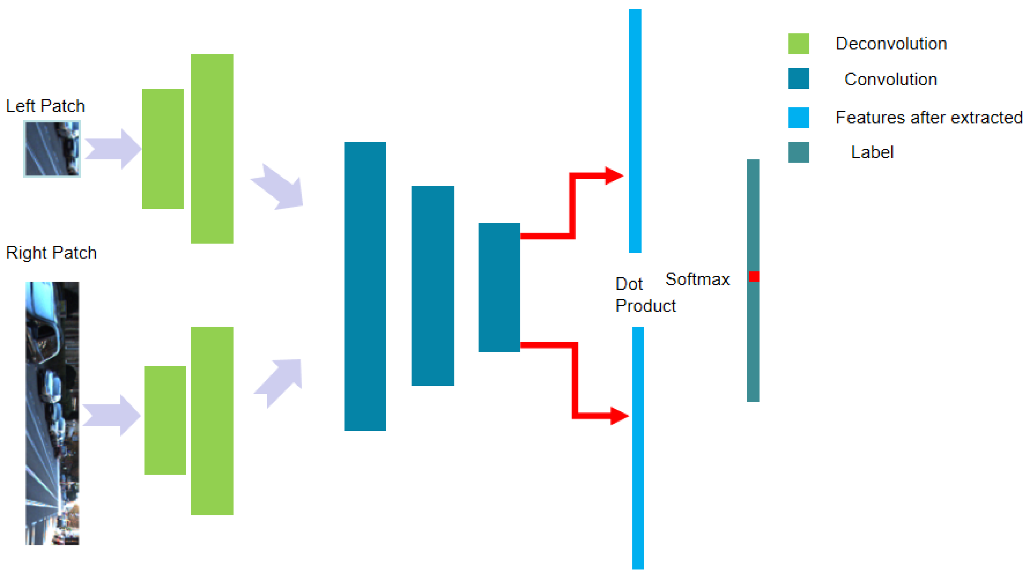
Figure 2.
Adaptive deconvolution-based disparity matching net (ADSM) network structure. This structure only consists of a convolutional layer and deconvolution layer. At the end, it compares the label with dot product produced by the extracted features.
Figure 2.
Adaptive deconvolution-based disparity matching net (ADSM) network structure. This structure only consists of a convolutional layer and deconvolution layer. At the end, it compares the label with dot product produced by the extracted features.
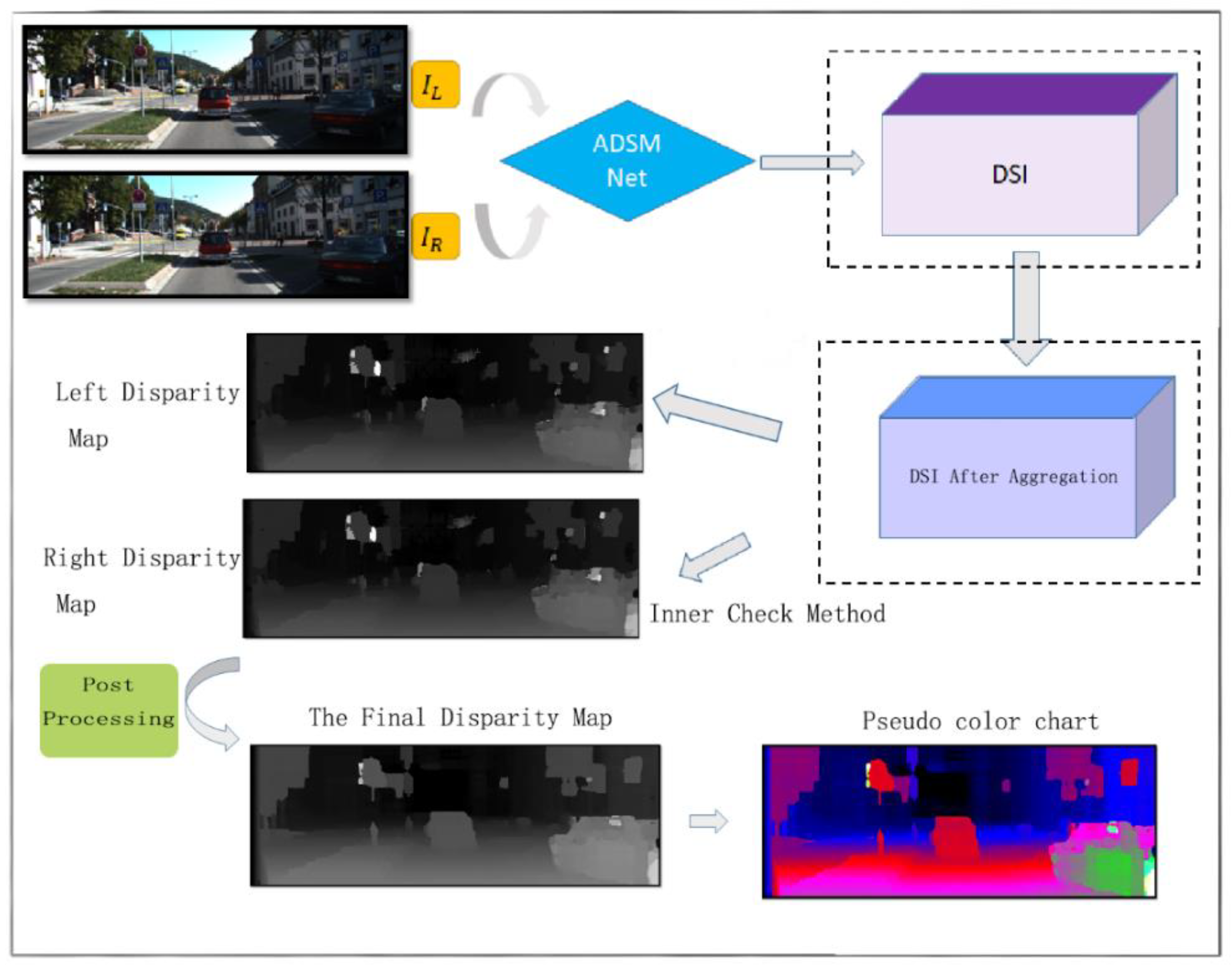
Figure 3.
The overall structure of the stereo matching algorithm. The left and right image will pass through ASDM Net and generate a three-dimensional array called the DSI (disparity space image). After four-way cost aggregation, a new DSI will be generated. In this paper, we will use the quadratic fitting method to directly attend the sub-pixel level. After that, we use the inner check method to check the left and right consistency and finally, use the ray filling method to fill the invalid pixel position.
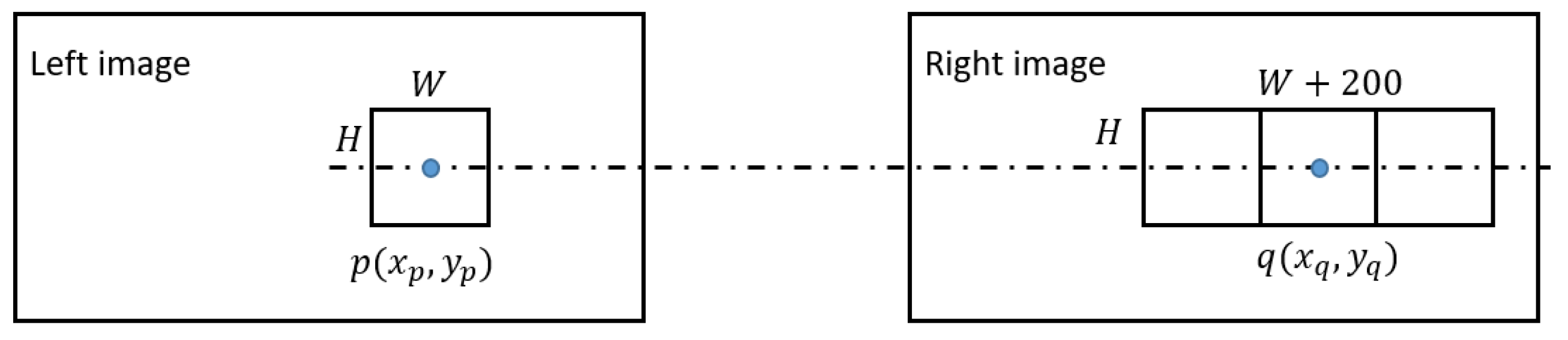
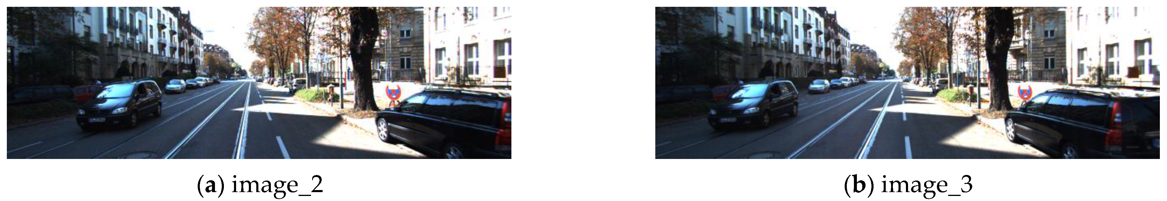
Figure 4.
Illustration of the input left and right image patches. Since the input images have been rectified by pole line, the center of the left and right image are all on the uniform line.
Figure 4.
Illustration of the input left and right image patches. Since the input images have been rectified by pole line, the center of the left and right image are all on the uniform line.
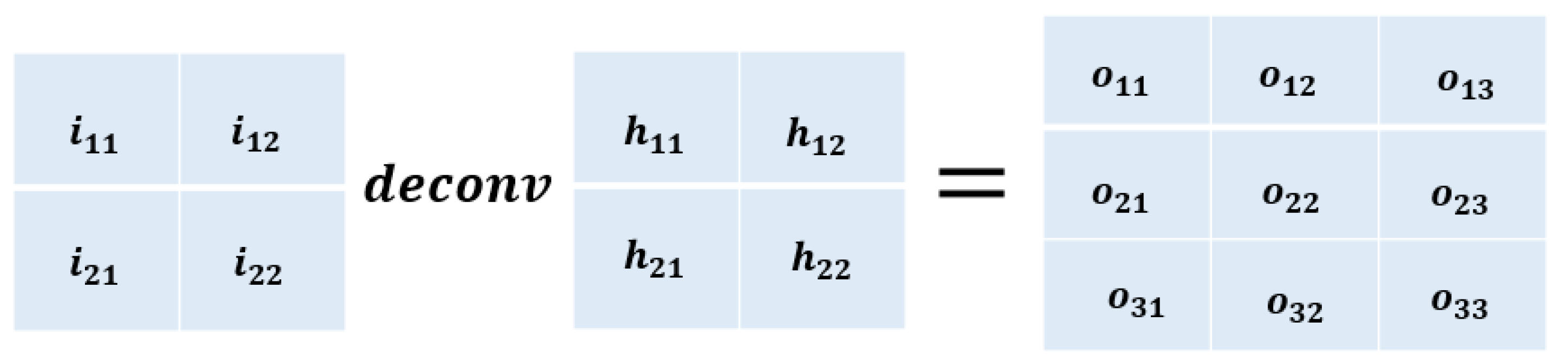
Figure 5.
The operation of the one-step of deconvolution. Deconvolution is similar to convolution except that it can enlarge the original image.
Figure 5.
The operation of the one-step of deconvolution. Deconvolution is similar to convolution except that it can enlarge the original image.
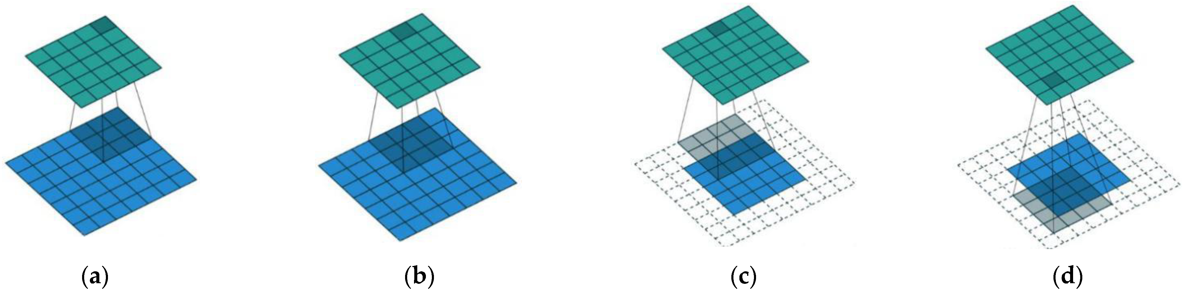
Figure 6.
Illustration of convolution and deconvolution. (a,b) represent the convolution operation, the green part represents the convolution result and blue part represents the input, the shadow part represents the size of convolution kernel. (c,d) represent the deconvolution operation, the green part represents the deconvolution result, the blue part represents the input and the shadow part represents the kernel of deconvolution.
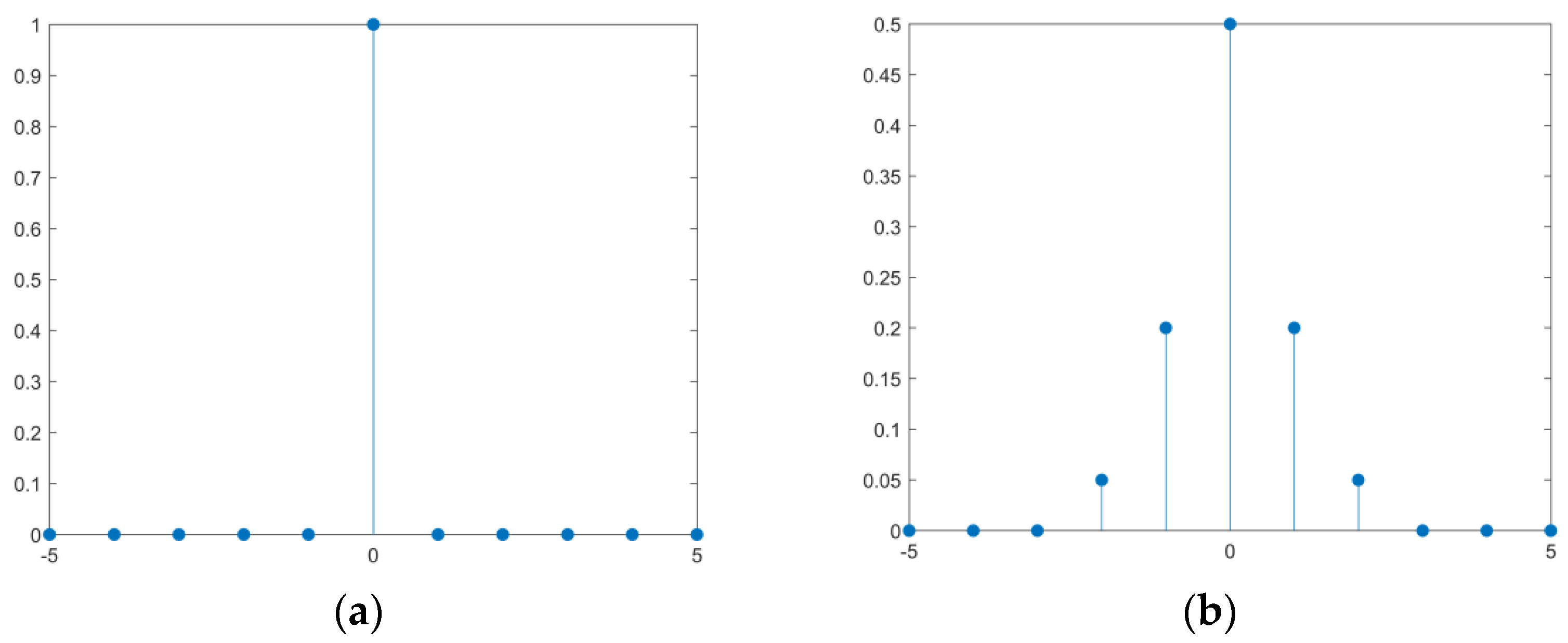
Figure 7.
(a,b) represent different weight values for calculating cross entropy loss.
Figure 7.
(a,b) represent different weight values for calculating cross entropy loss.
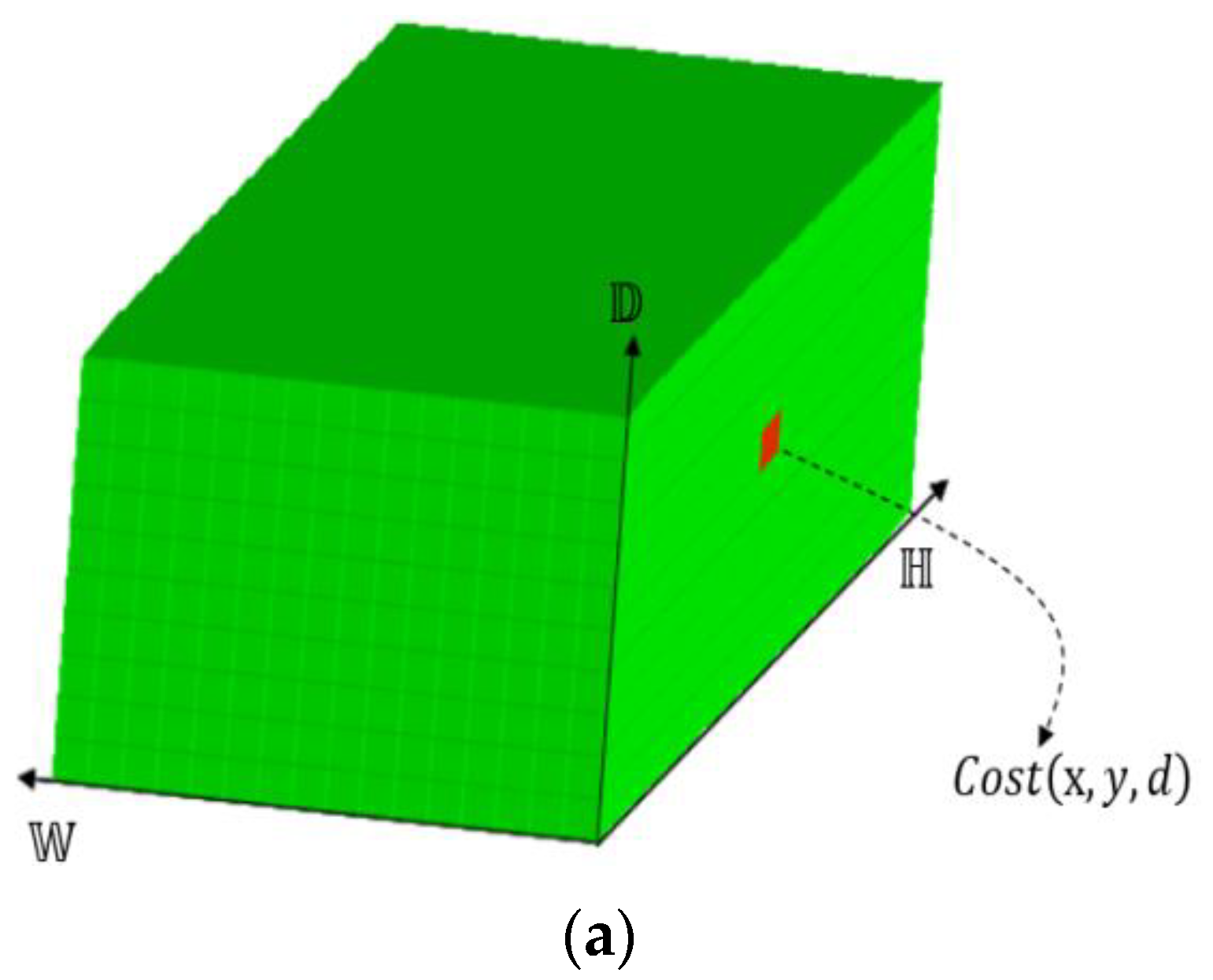
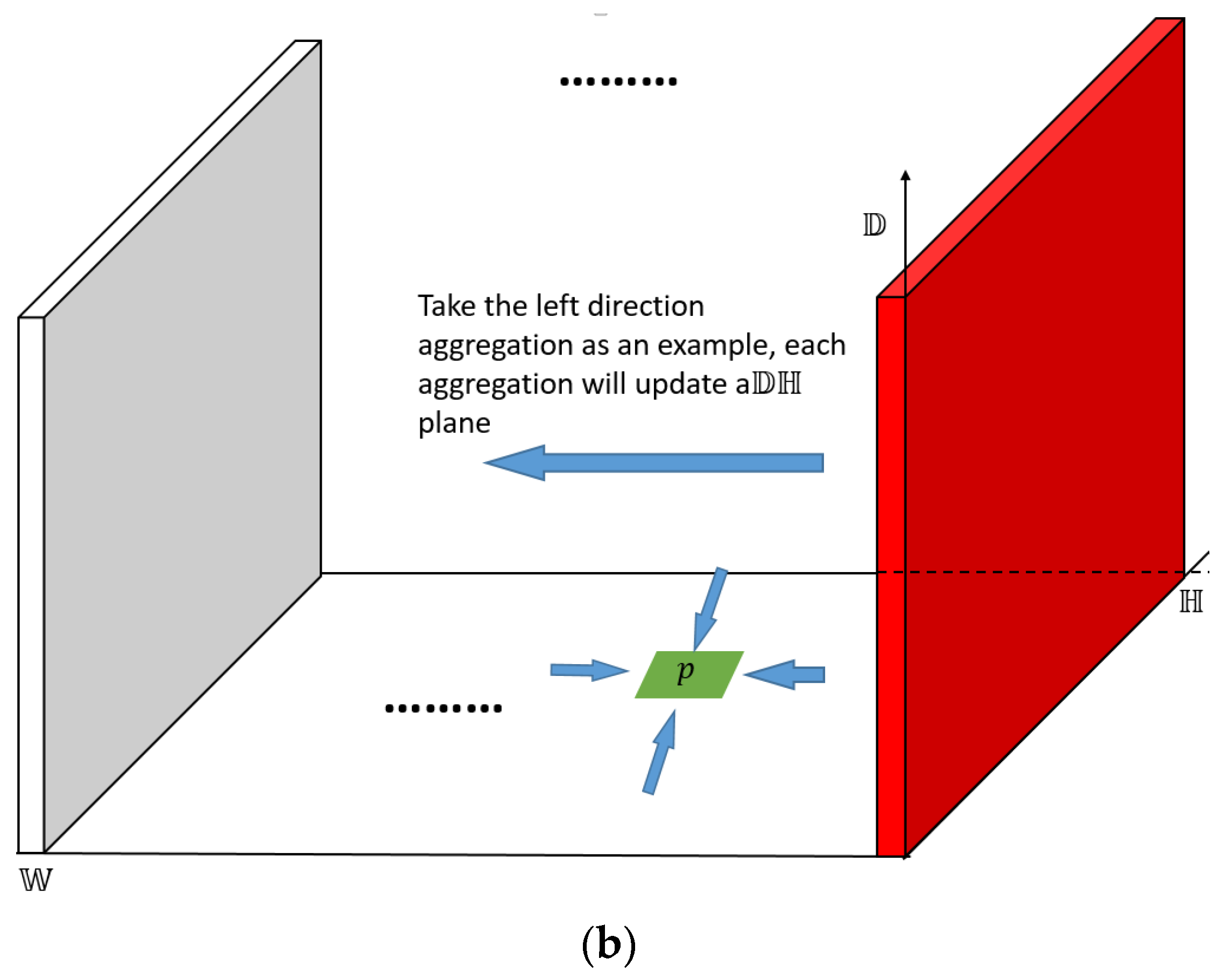
Figure 8.
Disparity space image-based aggregation illustration, (a) represents disparity space image, (b) represents aggregation along with the left horizontal direction.
Figure 8.
Disparity space image-based aggregation illustration, (a) represents disparity space image, (b) represents aggregation along with the left horizontal direction.
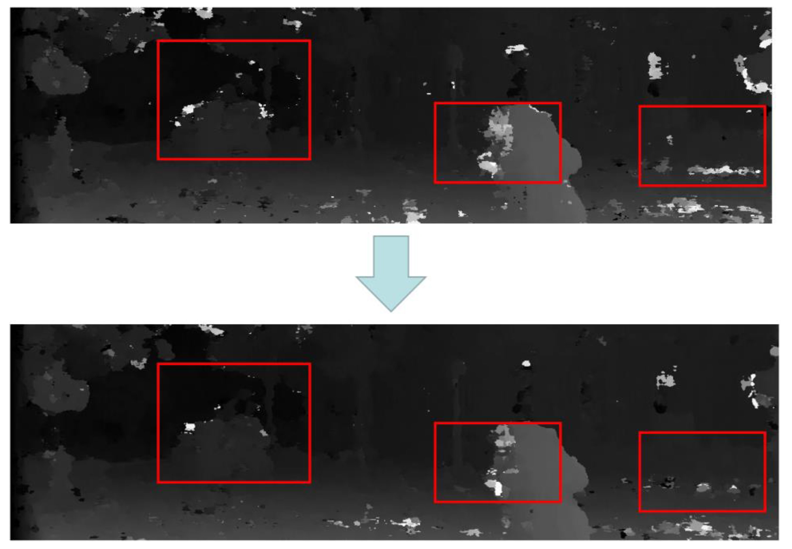
Figure 9.
The upper image was generated by the proposed neural network with 4Conv, the following image was generated by 1Deconv(5) and 4Conv. The input block size was set to be 37 × 37.
Figure 9.
The upper image was generated by the proposed neural network with 4Conv, the following image was generated by 1Deconv(5) and 4Conv. The input block size was set to be 37 × 37.
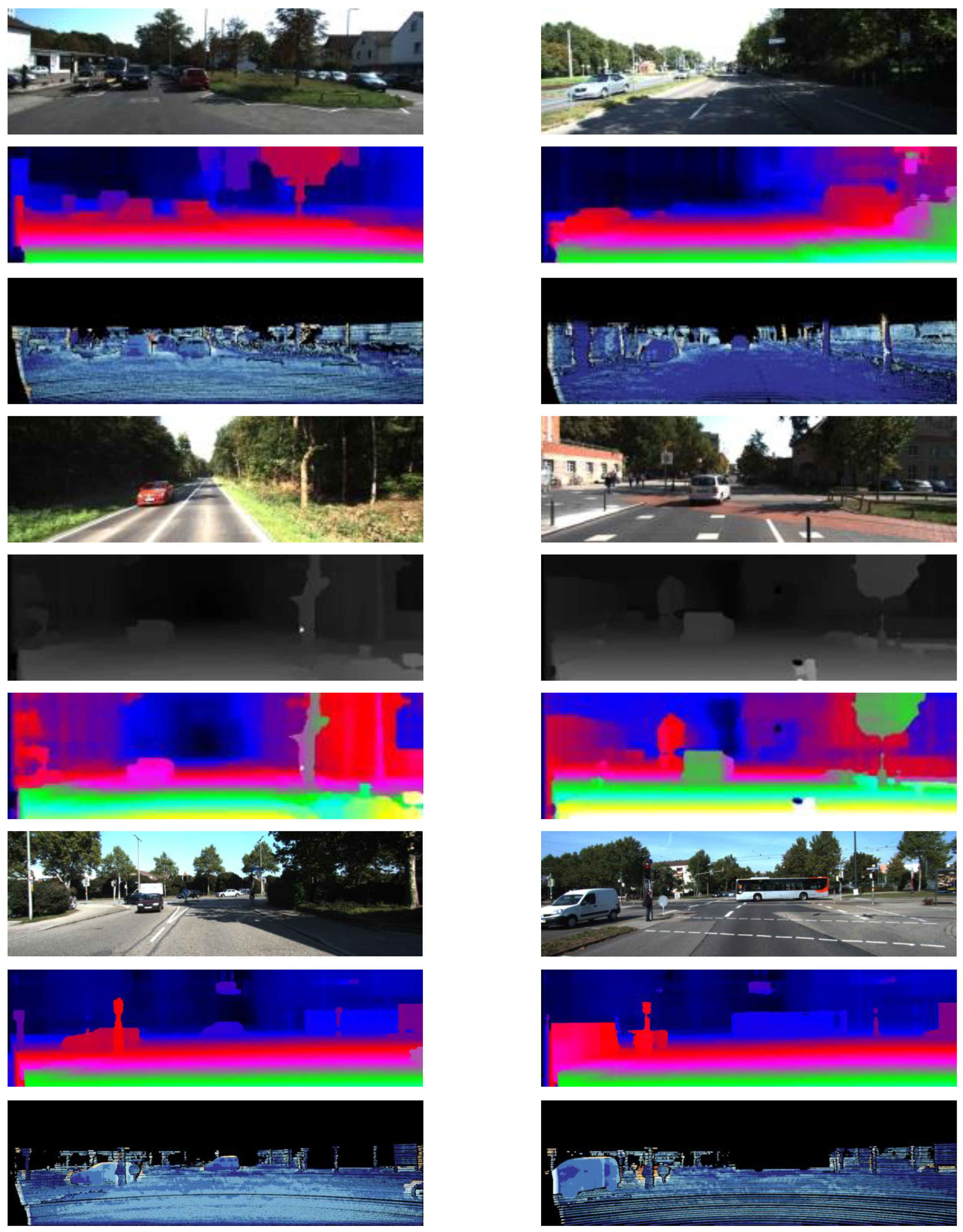
Figure 10.
Sample images of KITTI2015 dataset.
Figure 10.
Sample images of KITTI2015 dataset.
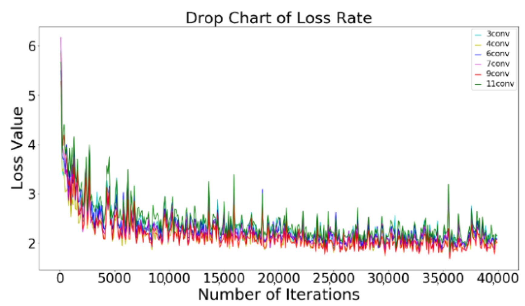
Figure 11.
Loss curve of different network configurations.
Figure 11.
Loss curve of different network configurations.
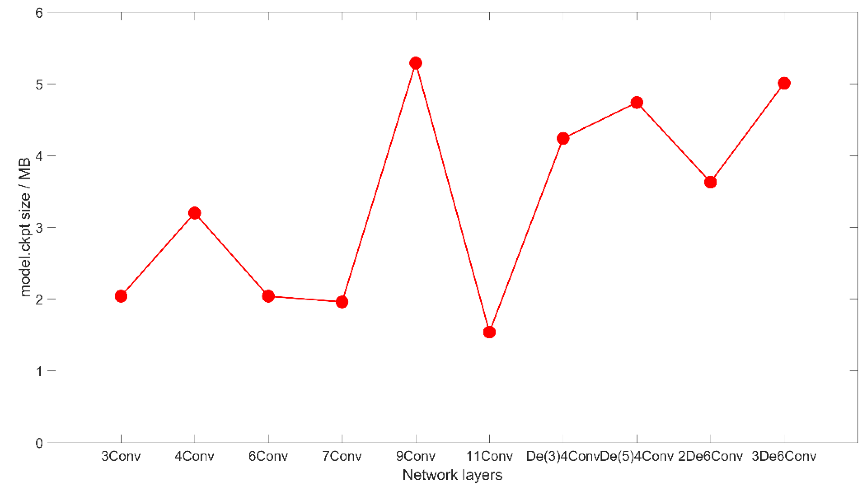
Figure 12.
The network model (model.ckpt file) size after training for different network structures. The ckpt file is a binary file from tensoflow, which stores all the weights, bias, gradients and other variables.
Figure 12.
The network model (model.ckpt file) size after training for different network structures. The ckpt file is a binary file from tensoflow, which stores all the weights, bias, gradients and other variables.
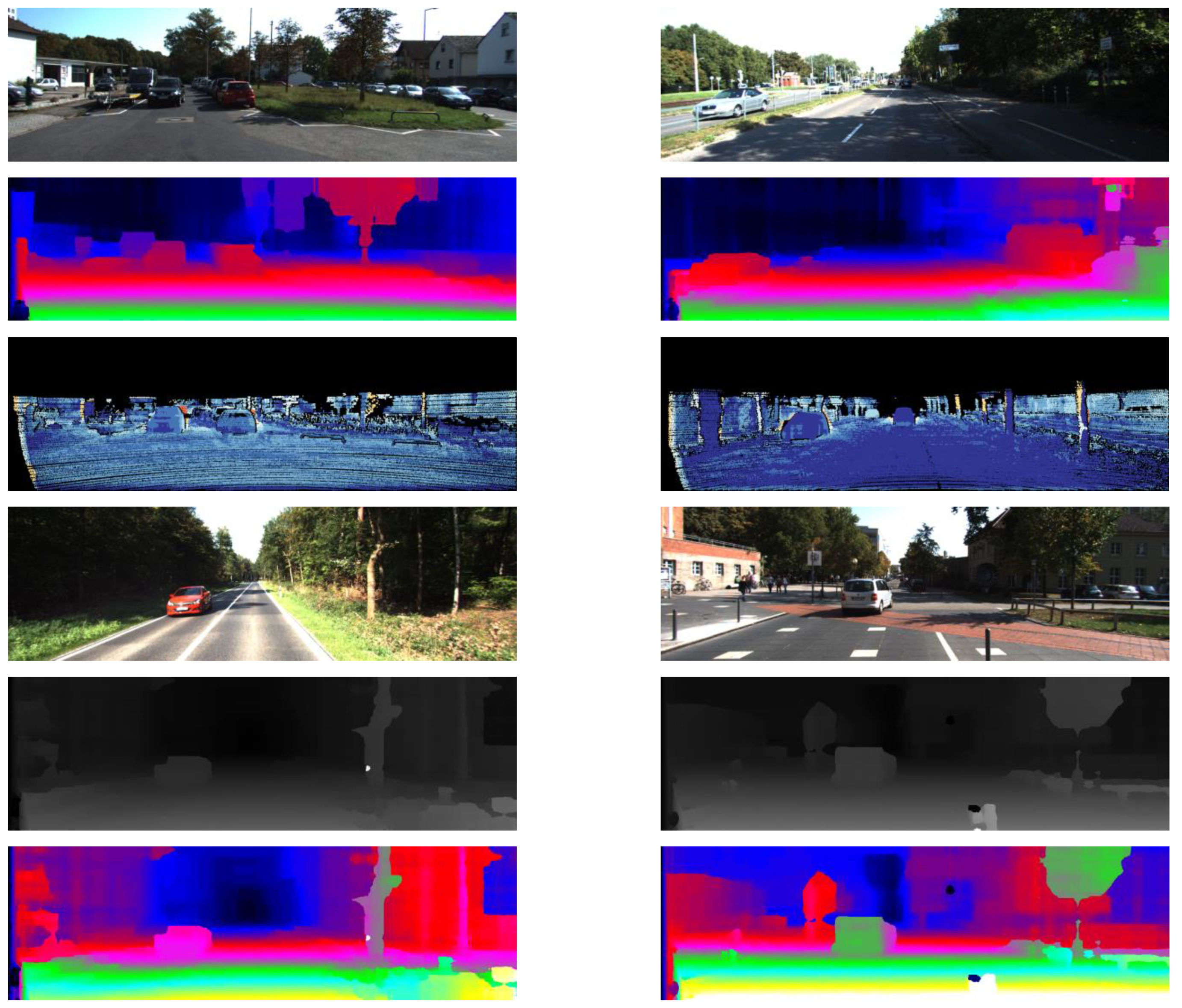
Figure 13.
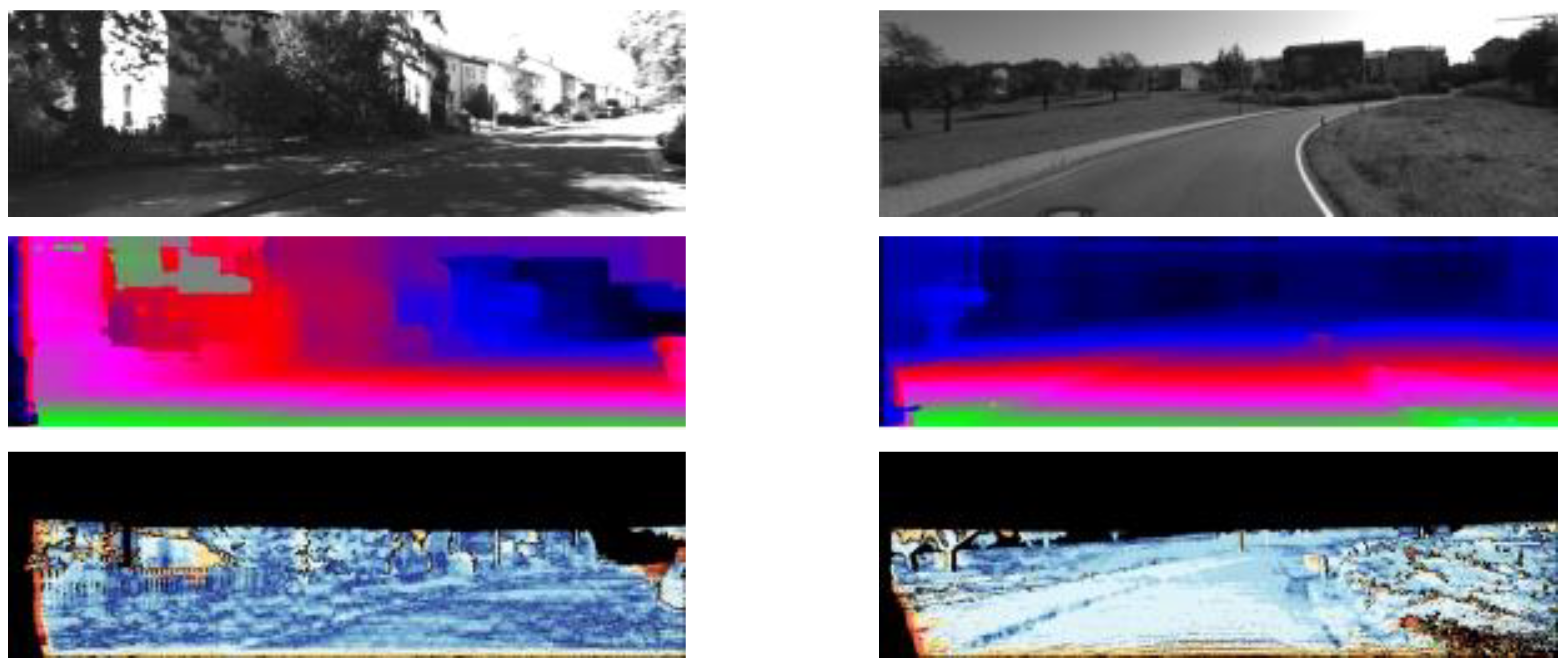
KITTI2015 test set: (top) original image, (center) stereo estimates, (bottom) stereo errors.
Figure 13.
KITTI2015 test set: (top) original image, (center) stereo estimates, (bottom) stereo errors.
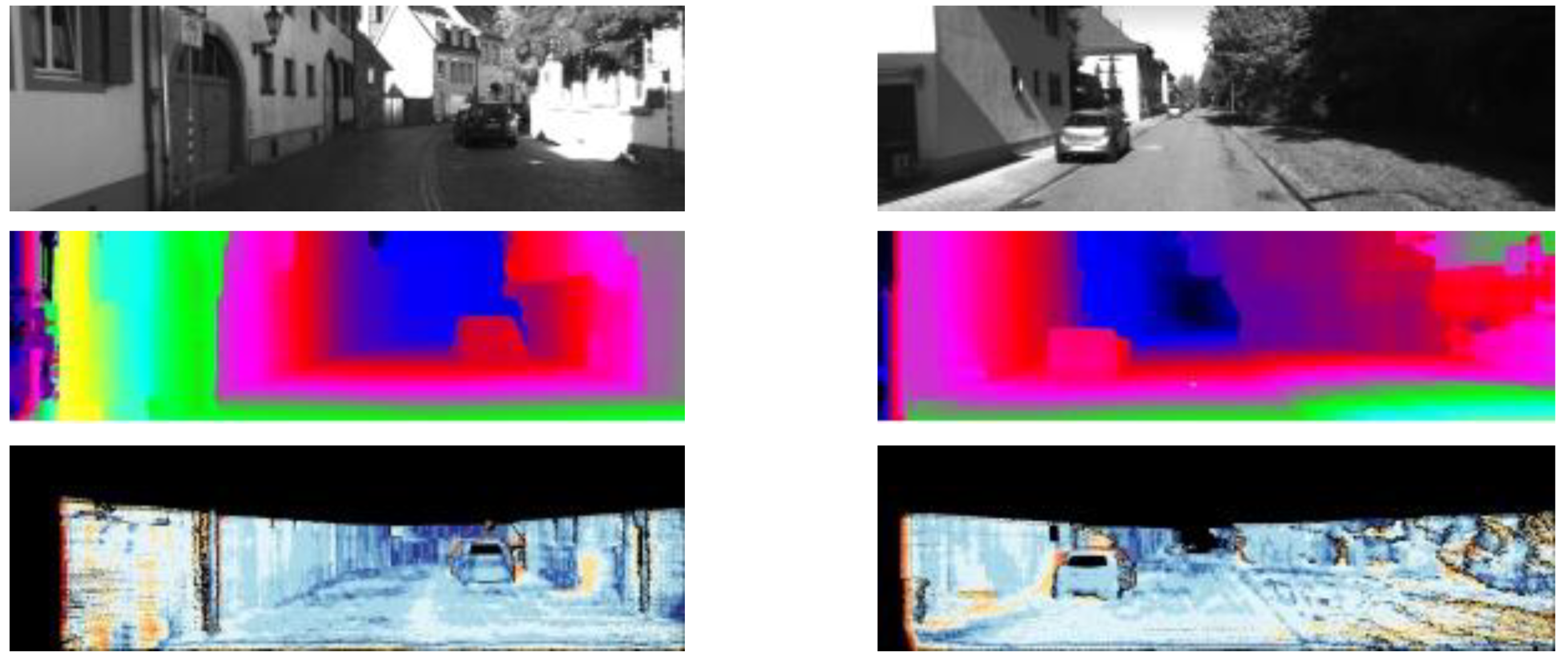
Figure 14.
KITTI2012 test set: (top) original image, (center) stereo estimates, (bottom) stereo errors.
Figure 14.
KITTI2012 test set: (top) original image, (center) stereo estimates, (bottom) stereo errors.
Table 1.
Six configurations of convolutional layers for the proposed neural network.
Table 1.
Six configurations of convolutional layers for the proposed neural network.
| 3Conv | 4Conv | 6Conv |
|---|
| Conv13 + BN + ReLU | Conv10 + BN + ReLU | Conv9 + BN + ReLU |
| Conv13 + BN + ReLU | Conv10 + BN + ReLU | Conv9 + BN + ReLU |
| Conv13 + softmax | Conv10 + BN + ReLU | Conv7 + BN + ReLU |
| | Conv10 + softmax | Conv7 + BN + ReLU |
| | | Conv5 + BN + ReLU |
| | | Conv5 + softmax |
| 7Conv | 9Conv | 11Conv |
| Conv7 + BN + ReLU | Conv5 + BN + ReLU | Conv5 + BN + ReLU |
| Conv7 + BN + ReLU | Conv5 + BN + ReLU | Conv5 + BN + ReLU |
| Conv7 + BN + ReLU | Conv5 + BN + ReLU | Conv5 + BN + ReLU |
| Conv7 + BN + ReLU | Conv5 + BN + ReLU | Conv5 + BN + ReLU |
| Conv5 + BN + ReLU | Conv5 + BN + ReLU | Conv5 + BN + ReLU |
| Conv5 + BN + ReLU | Conv5 + BN + ReLU | Conv5 + BN + ReLU |
| Conv5 + softmax | Conv5 + BN + ReLU | Conv5 + BN + ReLU |
| | Conv5 + BN + ReLU | Conv3 + BN + ReLU |
| | Conv5 + softmax | Conv3 + BN + ReLU |
| | | Conv3 + BN + ReLU |
| | | Conv3 + softmax |
Table 2.
The overall convolution neural network configurations for the proposed neural network.
Table 2.
The overall convolution neural network configurations for the proposed neural network.
| 1Deconv(5) and 4Conv | 1Deconv(3) and 4Conv | 2Deconv and 6Conv | 3Deconv and 6Conv |
|---|
| Deconv5 + BN | Deconv3 + BN | Deconv3 + BN | Deconv3 + BN + ReLU |
| Conv11 + BN + ReLU | Conv11 + BN + ReLU | Deconv5 + BN | Deconv5 + BN + ReLU |
| Conv11 + BN + ReLU | Conv11 + BN + ReLU | Conv9 + BN + ReLU | Deconv7 + BN + ReLU |
| Conv11 + BN + ReLU | Conv10 + BN + ReLU | Conv9 + BN + ReLU | Conv9 + BN + ReLU |
| Conv11 + softmax | Conv10 + softmax | Conv9 + BN + ReLU | Conv9 + BN + ReLU |
| | | Conv7 + BN + ReLU | Conv9 + BN + ReLU |
| | | Conv7 + BN + ReLU | Conv7 + BN + ReLU |
| | | Conv7 + softmax | Conv7 + BN + ReLU |
| | | | Conv7 + softmax |
Table 3.
The percentage of missing matching pixels with threshold of 2, 3, 4, 5 in the 2015 KITTI test set.
Table 3.
The percentage of missing matching pixels with threshold of 2, 3, 4, 5 in the 2015 KITTI test set.
| ConvNet-ValError | 2-Pixel-Error | 3-Pixel-Error | 4-Pixel-Error | 5-Pixel-Error |
|---|
| 37-3Conv | 12.21 | 8.55 | 6.95 | 6.05 |
| 37-4Conv | 11.11 | 8.12 | 6.82 | 6.01 |
| 37-6Conv | 11.79 | 8.73 | 8.35 | 6.53 |
| 37-7Conv | 11.96 | 8.87 | 7.53 | 6.73 |
| 37-9Conv | 10.86 | 8.07 | 6.82 | 6.07 |
| 37-11Conv | 14.95 | 10.36 | 8.82 | 7.92 |
Table 4.
The number of network parameters of different network structures for input left patch size 37.
Table 4.
The number of network parameters of different network structures for input left patch size 37.
| NetworkType | 3Conv | 4Conv | 6Conv | 7Conv | 9Conv | 11Conv |
|---|
| Number of unilateral network parameters | 1,416,896 | 1,248,000 | 953,536 | 918,720 | 721,600 | 627,932 |
Table 5.
The number of network parameters with deconvolution structure for input left patch size 37.
Table 5.
The number of network parameters with deconvolution structure for input left patch size 37.
| Network Type | 1Deconv(5) and 4Conv | 1Deconv(3) and 4Conv | 2Deconv and 6Conv | 3Deconv and 6Conv |
|---|
| Number of unilateral network parameters | 1,987,264 | 1,812,160 | 1,701,568 | 1,902,182 |
Table 6.
The results with deconvolution structure and other network for input left patch size 37.
Table 6.
The results with deconvolution structure and other network for input left patch size 37.
| ConvNet-ValError | 2-Pixel-Error | 3-Pixel-Error | 4-Pixel-Error | 5-Pixel-Error |
|---|
| 37-1Deconv(5) and 4Conv | 10.31 | 7.60 | 6.38 | 5.74 |
| 37-1Deconv(3) and 4Conv | 10.36 | 7.67 | 6.49 | 5.78 |
| 37-2Deconv and 6Conv | 13.63 | 10.56 | 9.27 | 8.53 |
| 37-3Deconv and 6Conv | 15.65 | 12.46 | 11.17 | 10.45 |
| MC-CNN-acrt [19] | 15.02 | 12.99 | 12.04 | 11.38 |
| MC-CNN-fast [19] | 18.47 | 14.96 | 13.18 | 12.02 |
| Efficient-Net [18] | 11.67 | 8.97 | 7.62 | 6.78 |
Table 7.
The percentage of missing matching pixels with threshold of 2, 3, 4, 5 in the 2015 KITTI test set for input left patch size 29, 33, 41, 45.
Table 7.
The percentage of missing matching pixels with threshold of 2, 3, 4, 5 in the 2015 KITTI test set for input left patch size 29, 33, 41, 45.
| Input Patch Size | ConvNetModel | 2-Pixel-Error | 3-Pixel-Error | 4-Pixel-Error | 5-Pixel-Error |
|---|
| | 3Conv | 13.49 | 10.29 | 8.79 | 7.92 |
| | 4Conv | 12.76 | 9.98 | 8.63 | 7.84 |
| | 5Conv | 12.8 | 10.1 | 8.78 | 8.03 |
| 29 × 29 | 7Conv | 13.21 | 10.44 | 9.13 | 8.36 |
| | 1Deconv(3)-4Conv | 12.47 | 9.89 | 8.71 | 8.02 |
| | 1Deconv(2)-4Conv | 12.96 | 10.28 | 9.04 | 8.32 |
| | 4Conv | 12.34 | 9.59 | 8.25 | 7.45 |
| | 8Conv | 13.11 | 10.31 | 8.63 | 7.84 |
| 33 × 33 | 1Deconv(3)-4Conv | 12.20 | 9.70 | 8.55 | 7.88 |
| | 1Deconv(5)-4Conv | 12.80 | 10.20 | 9.03 | 8.35 |
| | 4Conv | 10.61 | 7.69 | 6.41 | 5.66 |
| | 5Conv | 10.39 | 7.64 | 6.43 | 5.69 |
| | 8Conv | 11.03 | 8.21 | 6.96 | 6.21 |
| 41 × 41 | 10Conv | 11.47 | 8.51 | 7.21 | 6.45 |
| | 1Deconv(3)-4Conv | 9.94 | 7.31 | 6.15 | 5.47 |
| | 1Deconv(5)-4Conv | 10.26 | 7.51 | 6.29 | 5.56 |
| | 4Conv | 10.48 | 7.55 | 6.24 | 5.47 |
| 45 × 45 | 5Conv | 10.54 | 7.69 | 6.44 | 5.69 |
| | 8Conv | 10.78 | 7.88 | 6.62 | 5.85 |
| | 1Deconv(3)-4Conv | 9.45 | 6.86 | 5.72 | 5.03 |
Table 8.
The percentage of missing matching pixels with thresholds of 2, 3, 4, 5 in the 2012 KITTI validation set.
Table 8.
The percentage of missing matching pixels with thresholds of 2, 3, 4, 5 in the 2012 KITTI validation set.
| ConvNetModel | 2-Pixel-Error | 3-Pixel-Error | 4-Pixel-Error | 5-Pixel-Error |
|---|
| MC-CNN-acrt [21] | 16.92 | 14.93 | 13.98 | 13.32 |
| MC-CNN-fast [21] | 19.56 | 17.41 | 16.31 | 15.51 |
| Efficient-Net [15] | 12.86 | 10.64 | 9.65 | 9.03 |
| Ours | 8.42 | 7.07 | 6.43 | 6.02 |
Table 9.
Error comparison of disparity with different algorithms (KITTI2012) %.
Table 9.
Error comparison of disparity with different algorithms (KITTI2012) %.
| Algorithm | 2-Pixel-Error | 3-Pixel-Error | 4-Pixel-Error | 5-Pixel-Error | Runtime (s) |
|---|
| StereoSLIC [31] | 7.20 | 5.11 | 4.04 | 3.33 | 2.3 |
| PCBP-SS [30] | 6.75 | 4.72 | 3.75 | 3.15 | 300 |
| SPSS [30] | 6.28 | 4.41 | 3.52 | 3.00 | 2 |
| MC-CNN-acrt [19] | 5.45 | 3.63 | 2.85 | 2.39 | 67 |
| Displets v2 [32] | 4.46 | 3.09 | 2.52 | 2.17 | 265 |
| Efficient-CNN [18] | 6.51 | 4.29 | 3.36 | 2.82 | 0.7 |
| Ours | 5.62 | 4.01 | 3.02 | 2.65 | 2.4 |
Table 10.
Error comparison of disparity with different algorithms (KITTI2015) %.
Table 10.
Error comparison of disparity with different algorithms (KITTI2015) %.
| Algorithm | 2-Pixel-Error | 3-Pixel-Error | 4-Pixel-Error | 5-Pixel-Error | Runtime (s) |
|---|
| Elas [28] | 24.09 | 19.21 | 17.59 | 16.82 | 0.669 |
| SGM [20] | 10.03 | 6.93 | 5.47 | 4.48 | 1.8 |
| SPSS [30] | 7.15 | 4.58 | 3.46 | 2.93 | 3 |
| Efficient-CNN [18] | 6.78 | 4.38 | 2.56 | 2.03 | 1 |
| MC-CNN-fast [19] | 7.53 | 4.01 | 2.84 | 2.33 | 0.2 |
| MC-CNN-slow [19] | 6.38 | 3.27 | 2.37 | 1.97 | 35 |
| Ours | 4.27 | 3.85 | 2.57 | 2.00 | 2.5 |


