Article

Fault-Tolerant Control Scheme for the Sensor Fault in the Acceleration Process of Variable Cycle Engine

College of Energy and Power Engineering, Nanjing University of Aeronautics and Astronautics, Nanjing 210016, China
*
Author to whom correspondence should be addressed.
Appl. Sci. 2022, 12(4), 2085; https://doi.org/10.3390/app12042085
Submission received: 28 January 2022 / Revised: 8 February 2022 / Accepted: 15 February 2022 / Published: 17 February 2022
(This article belongs to the Special Issue Advancing Reliability & Prognostics and Health Management)

Abstract

:
This paper presents a fault-tolerant control scheme for the sensor fault in the acceleration process of the variable cycle engine. Firstly, an adaptive equilibrium manifold model with multiple inputs and multiple outputs is established. Combined with the Kalman filter bank, sensor fault diagnosis is carried out to realize the diagnosis and signal reconstruction of the engine in the case of a single sensor and double sensor faults. On this basis, isolation and group isolation are used to diagnose sensor faults and reconstruct signal in speed closed-loop control. Then, the control plan of the acceleration process is optimized based on the target shooting method, aiming to simulate the variation of various variables in the engine acceleration process more accurately, so as to verify the feasibility of the sensor fault-tolerant control scheme. Finally, a hardware-in-loop simulation platform is built based on the idea of distributed control, and the fault-tolerant control scheme of the sensor proposed previously is verified based on this platform. The results show that the proposed scheme can accurately diagnose the sensor faults and reconstruct the signal within 0.2 s, and the actual speed can rise from 67.87% to 99.9% in 4 s, ensuring the safe and rapid completion of the acceleration process.

1. Introduction

As the “brain” of an aeroengine, the role of the control system is to make the engine work stably and reliably under any changing conditions and give full play to its performance benefits [1]. Visible, stability and reliability are the fundamental guarantee of all other higher control requirements. Modern aero engines adopt a full authority digital electronic control (FADEC) system responsible for complex tasks including control, monitoring and management. Its structure consists of numerous sensors, actuators and electronic control components. Due to the long-term work in high temperature, high pressure and intense vibration, these components are prone to failure during system operation. Once a fault occurs, the whole control system may collapse, resulting in severe consequences. According to the data, the sensor fault of aeroengine is higher than 80% of the total system fault [2].
Fault-tolerant control (FTC) means that when the system fails, the remaining control tasks can be completed safely according to the specified performance index, or the performance index can be reduced but still within the acceptable range. At present, the most fault-tolerant design of engine control systems is based on hardware redundancy. The development of non-hardware redundancy is mainly focused on sensor fault diagnosis and signal reconstruction. In the 1970s, Wallhagen, R. E. and D. J. Arpasi proposed a passive FTC technology with analytic redundancy to reconstruct the fault system for engines with sensor faults [3]. Since the 1980s, NASA has designed an analytical redundancy scheme to improve engine control reliability, which can detect and distinguish between hard and soft faults of the control system and reconstruct the system for sensor faults [4]. Around the 90s, Merrill et al. used a set of Kalman estimators in fault detection and isolation. By monitoring the residuals of each estimator, specific faults that have occurred can be detected and isolated [5,6]. Since the end of the last century, intelligent algorithms have been applied in sensor fault diagnosis and FTC systems and successfully verified in turbojet, turbofan and other engines [7,8]. Xianghua Huang used a self-association neural network to construct the analysis redundancy of sensors to ensure the reliability of aircraft engine closed-loop control [9]. Yang et al. used wavelet transform to diagnose sensor faults, and used BP neural network to predict the output data of fault sensors [10]. Zhao et al. obtained a set of modal functions by empirical mode decomposition of the output signal of the sensor, and took its sample entropy as the fault feature of the sensor, and classified the fault state of the sensor by sparse representation-based classifier [11]. Chen and Liu used radial basis function (RBF) neural network and general regression neural network (GRNN) respectively to predict timing data. If the difference between the predicted value and the actual output value of the sensor exceeds the set threshold, the sensor is considered to be faulty, and the sensor signal is reconstructed with the predicted value [12,13]. Sheng et al. proposed an intelligent FTC system based on an Online Sequential Extreme Learning Machine (OS-ELM) for sensor faults. The system can realize online fault diagnosis and signal reconstruction without establishing a system model [14]. These latest research results are mostly combined with artificial intelligence algorithm for sensor fault diagnosis, most of them stay at the theoretical level. The complexity of the algorithm reduces the speed of diagnosis and makes it difficult to apply it in engineering practice. Besides, most of the research on sensor FTC is based on steady-state control. In the process of engine transition, because the speed and other parameters are sensitive parameters closely related to the engine performance, to improve the stability and reliability of the transition, closed-loop control is often carried out. Therefore, the sensor FTC problem in the transition process also exists, but the relevant research is still relatively rare.
Because of this, this paper presents an acceleration control scheme based on fault tolerance of the sensor for variable cycle engine (VCE), as shown in Figure 1. First, in Section 2, an improved multi-input multi-output adaptive equilibrium manifold model (AEMM) with dual scheduling variables is established. In Section 3, the AEMM is combined with the Kalman filter bank to design the single sensor fault and the double sensor faults diagnosis scheme. Based on this, the actual engine parameter estimation under the sensor fault is obtained. In Section 4, A multi-target method is used to optimize the engine acceleration process control plan to verify the FTC scheme. In Section 5, the above procedure is verified by hardware-in-the-loop simulation, and the FTC of the accelerated process is proved from the perspective of engineering realizability. Section 6 concludes with a summary of the paper.

2. On-Board Adaptive Model

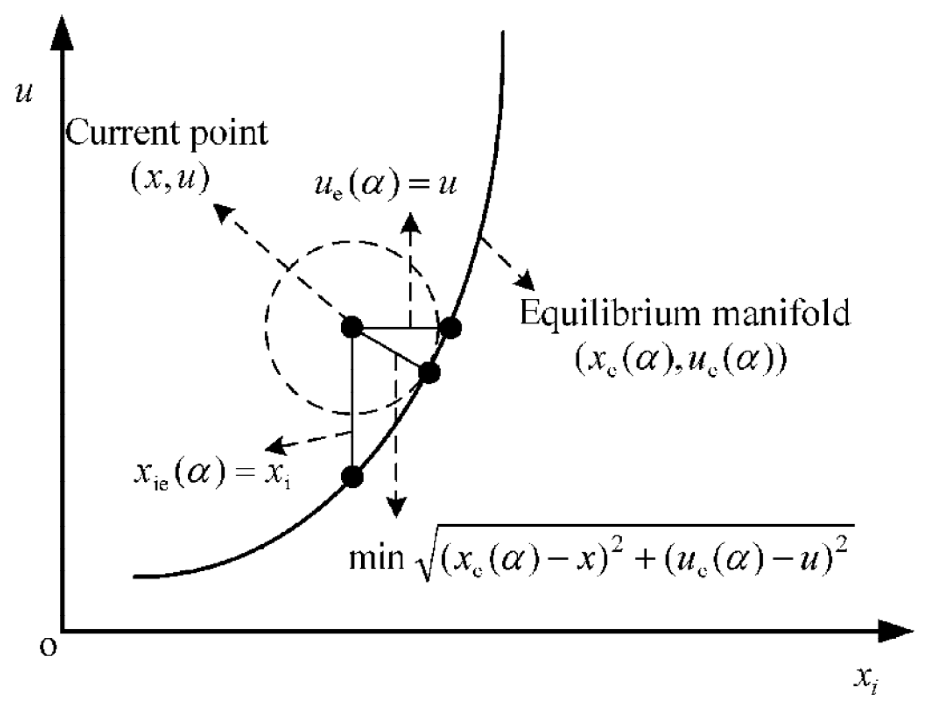
2.1. Equilibrium Manifold Model

Equilibrium manifold model (EMM) is a model developed from the linearization model [15].
Consider the following smooth nonlinear system:
x ˙ = f ( x , u ) y = g x , u ,
where f ( x , u ) and g ( x , u ) are smooth functions. Do Taylor expansion at any equilibrium point and abandon the higher-order terms, and a linear model of the original system can be obtained:
x ˙ = A x x e + B u u e y y e = C x x e + D u u e .
The set of all equilibrium points in a system constitutes an equilibrium family Γ e and Γ e can be considered an equilibrium manifold.
Γ e = x e , u e , y e | f x e , u e = 0 , y e = g x e , u e .
These equilibria can be scheduled with a variable of the same dimension as the control quantity u , which is defined as the scheduling variable α . α is composed of relevant variables of the current working point and can be expressed as α = p x , y , u . Then we can get:
x e = x e α u e = u e α y e = y e α .
Similarly, the state matrix and control matrix of the linearized model of the system at each equilibrium point can also be expressed as the matrix scheduled with α , so as to obtain the dynamic model of the system near the equilibrium manifold:
x ˙ = A α x x e α + B α u u e α y y e α = C α x x e α + D α u u e α .
To make the linearized model family (5) a nonlinear model, it is necessary to establish the relationship between scheduling variables α and the current working point. Considering the algebraic relationship between y and x , u , only the following design is needed:
α = p x , u .
By combining Equations (5) and (6), a nonlinear model scheduled by x and u can be obtained, that is, an equilibrium manifold model. It can be seen that the EMM is derived from the linearized model family (5) and the scheduling relation (6). It has the characteristic of variable parameter of linear parameter varying (LPV) model whose coefficient matrix all changes with the working state, and the introduction of Equation (4) makes the model always change near the equilibrium manifold, which overcomes the deficiency of steady-state error in LPV model.
In terms of the structure of the model, the EMM can be regarded as a Taylor expansion model at the equilibrium point of real-time change. The Equation (6) essentially establishes a mapping of the current operating point to the Taylor expansion point on the equilibrium manifold. Figure 2 shows the three mapping modes of equal input u = u e α , equal partial state x i = x i e α , and the orthogonal expansion x e α x 2 + u e α u 2 . The Equation (6) can be obtained from these mappings. The three designs have different EMM and different errors from Equation (1). Determine the value of the scheduling variable utilizing equal input shown in Figure 2 and select fuel flow W f and nozzle area A 8 as the scheduling variables. Then, there is W f e α = W f , A 8 e α = A 8 and α = W f , A 8 . Represent A α as a 11 ( α ) a 12 ( α ) a 21 ( α ) a 22 ( α ) and the EMM of the above process can be expressed as:
n ˙ h = a 11 α n h n h e α + a 12 α n l n l e α n ˙ l = a 21 α n h n h e α + a 22 α n h n l e α α = u = W f e , A 8 e .
It can be seen that, due to the selection of scheduling variables and scheduling relations, the control matrix B α will not appear in the equilibrium manifold expansion model, and the EMM is reduced to a group of differential equations without initial input. It should be noted that the complete dynamic matrix can be obtained by taking partial derivatives of the corresponding variables [16]. In other words, the EMM and the nonlinear model have the same state-space matrix at the same equilibrium point, that is, their linearization models are the same. Using this property, the B matrix at any equilibrium point can be obtained.
Due to the strong nonlinear characteristics of the engine, just as different input combinations can obtain different linearized models, a nonlinear object also has multiple equilibrium manifold dynamic structures, which means different combinations of inputs give different A α . That is to say, if a set of inputs is applied at a certain equilibrium point and identification data is obtained, then the identified model can only be used in the neighborhood of the set of inputs (i.e., the point with little state change). In addition, since the EMM loses the B matrix and only retains a matrix, different input combinations are easy to identify and obtain a matrix with great differences. Compared with the traditional MIMO linearization model, it is easier to generate dynamic characteristics with remarkable differences. To solve this problem, one way is to build different EMMs for different input combinations. We can define the following variables:
θ = Δ W f / W f Δ W f / W f + Δ A 8 / A 8 ,
where W f and A 8 represent the length of the subinterval, Δ W f and Δ A 8 represent the change value of the input quantity. Therefore, this variable can be regarded as the proportion of the change of fuel flow in the shift of total input quantity and can be called the modification of control quantity.
Then the EMM of the engine with a wide range of variable cycles can be obtained through identification and the parameterized representation of the model coefficient matrix under each θ [17]. It should be noted that parameter identification of coefficient matrix needs to be based on nonlinear component level model (CLM) of the engine. The establishment method of CLM of VCE has been very mature. For example, detailed steps are given in reference [18], which will not be elaborated in detail in this paper.
The following is to test the operation effect of the model by changing the control quantity randomly in an extensive range. The control quantity shown in Figure 3 is applied to the CLM and the EMM. The operation results of the two models are shown in Figure 4. It can be seen that the model has high steady-state accuracy and good dynamic accuracy.

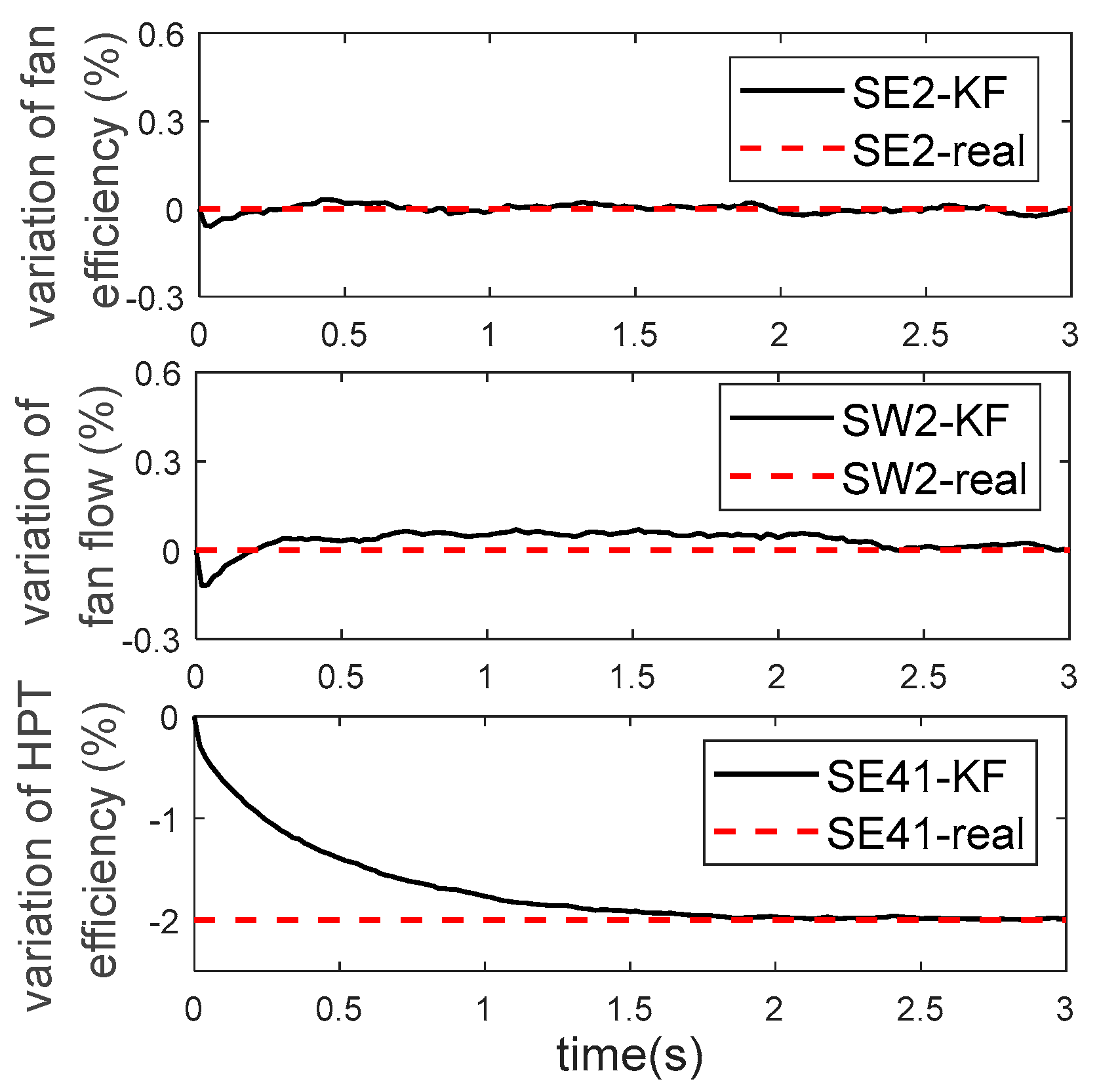
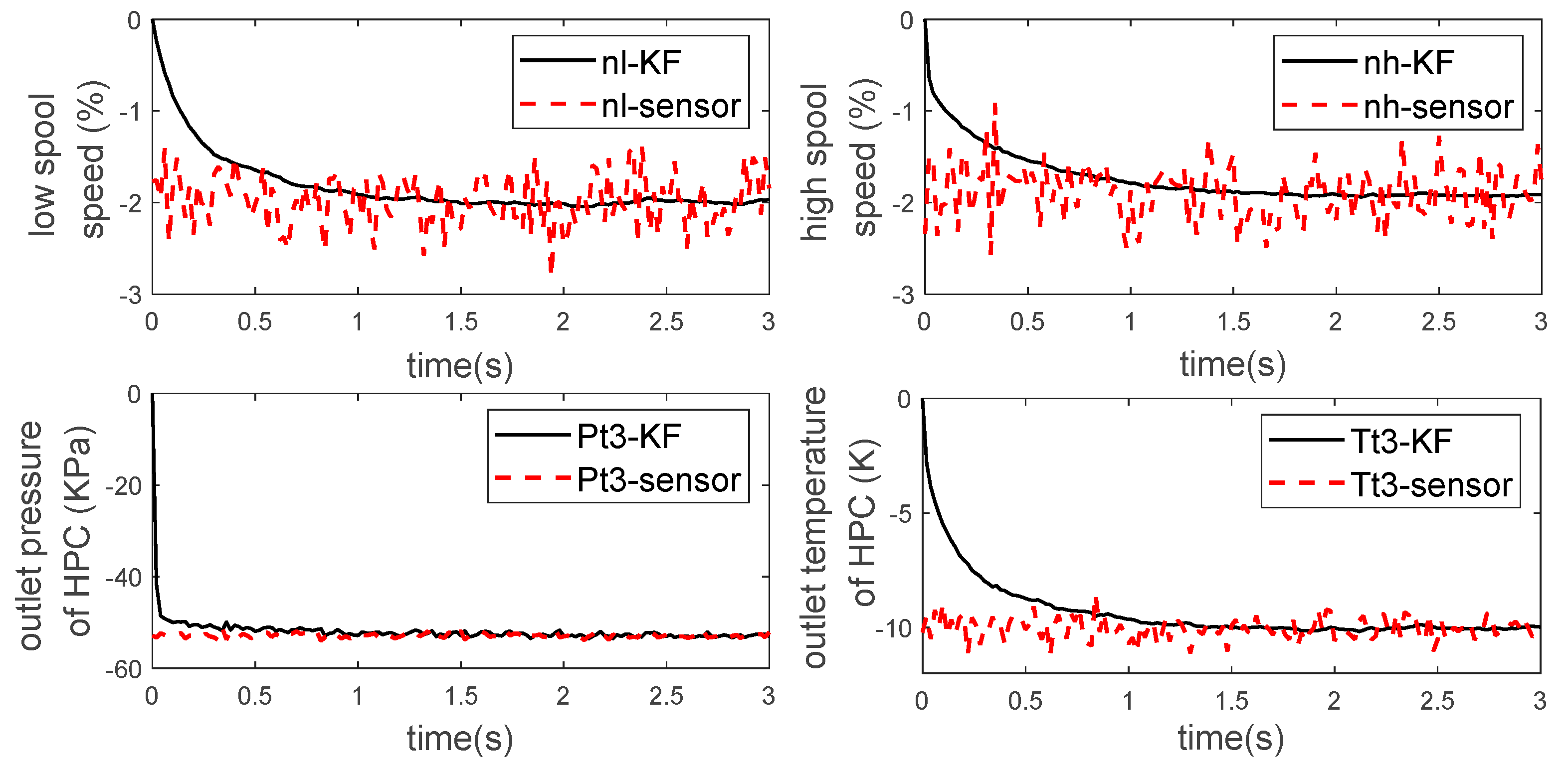
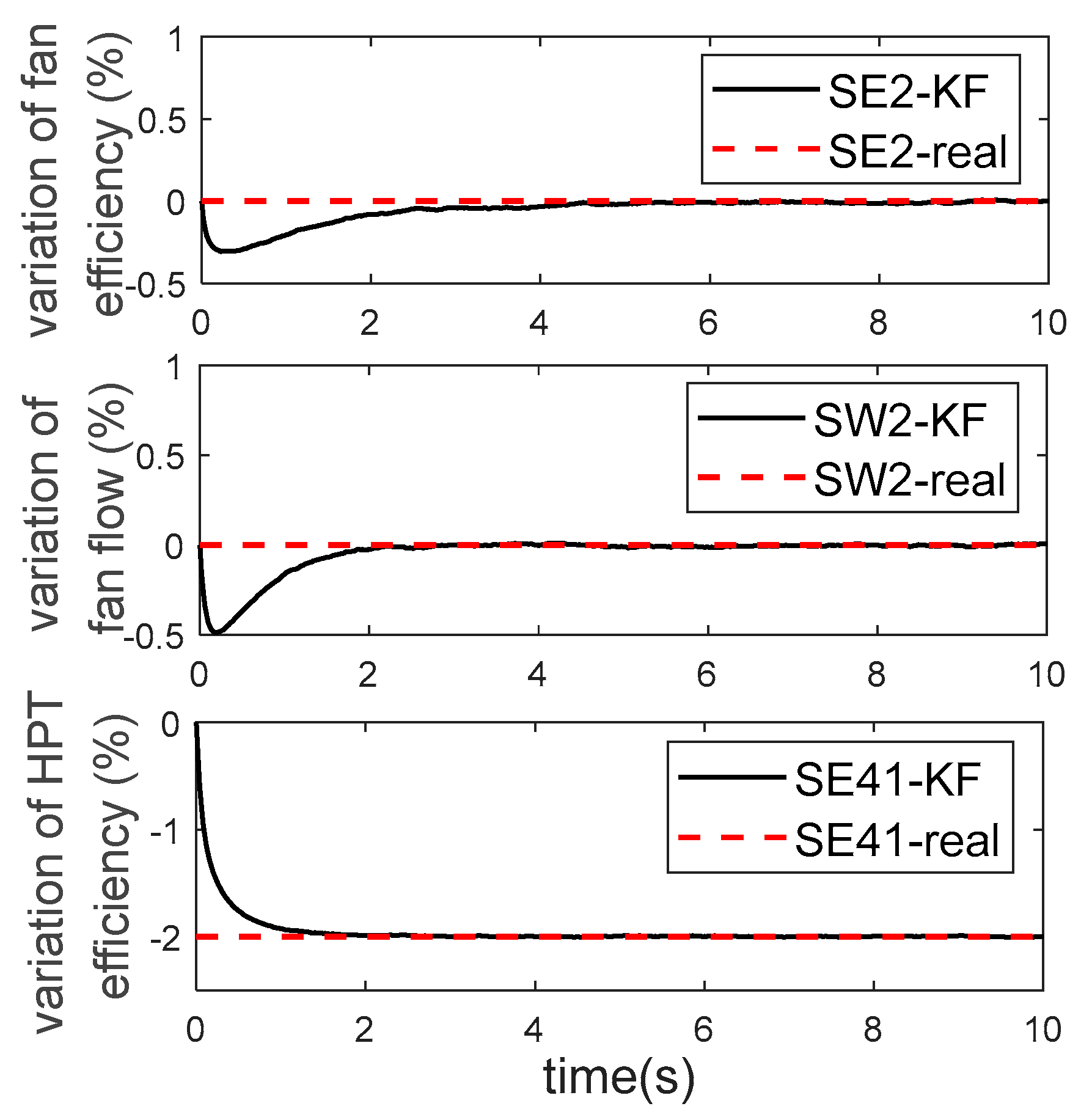
2.2. On-Board Adaptive Equilibrium Manifold Model

Referring to the conventional linear state variable model with degradation, the following EMM with degradation is established:
x ˙ = A α x x e α + L α h y y e α = C α x x e α + M α h ,
where h is the engine health parameter, representing the degradation of the flow/efficiency of each engine component. α is the scheduling variable. Since the health parameters are independent of the scheduling variables, they are not scheduled by them, while the coefficient matrices L and M are related to the engine operating points and are scheduled by the scheduling variables.
Considering that performance degradation is a slow development process during the service period of the engine, it does not require high dynamic characteristics and focuses on its steady-state value. Therefore, based on the EMM without degradation, the matrix expressions are retained, and the health parameters are changed in the component level model to cause changes in state quantities and output quantities. The degradation coefficient matrices L(α) and M(α) are obtained by the changing steady-state values identification to form the final EMM with degradation.
An EMM with degradation is not enough to be called an adaptive model. It needs to have the ability to update health parameters (degradation) to match with the actual engine running state. For this reason, a Kalman filter is introduced to estimate the starter degradation from the measurable output deviation containing the measured noise. Firstly, model (9) is written into a standard form. For this reason, the health parameters are extended to state quantities.
x ˙ h ˙ = A a u g x x e α h + ω y y e α = C a u g x x e α h + υ ,
where A a u g = A α L α 0 0 and C a u g = C α M α . ω and υ are the system noise matrix and measurement noise matrix respectively, and the covariance matrices are Q and R . Then, the Kalman filter uses the probability distribution of the measured value and the optimal estimate to obtain the optimal state estimate:
x ^ ˙ h ^ ˙ = A a u g x ^ x e α h ^ + K y y ^ y ^ y e α = C a u g x ^ x e α h ^ ,
where x ^ , y ^ , h ^ are estimated values of state quantity, output quantity and degradation quantity. K is called the Kalman filter gain, and K = P C a u g R 1 . P is the solution of the following Riccati equation:
A a u g P + P A a u g T P C a u g T R 1 C aug P + Q = 0 .
Thus, the AEMM is formed. The ability of health parameter estimation of this model is verified at the design point below. Set high-pressure turbine component efficiency in degrading by 2%, and the steady-state deviation of the output of the CLM and the output without degradation is respectively Δ n l = 1.98 % , Δ n h = 1.93 % , Δ P t 3 = 52.84 Kpa and Δ T t 3 = 10.0 K. The steady-state output is added with Gaussian noise and fed into the Kalman filter to obtain the optimal estimation of health parameters and measured values, as shown in Figure 5 and Figure 6.
It can be seen that the Kalman filter can accurately estimate the efficiency degradation of the high-pressure turbine components at 2% within 1.5 s, and the estimation accuracy of other health parameters is also within 0.1%. At the same time, the estimation of the measured values also has high accuracy.

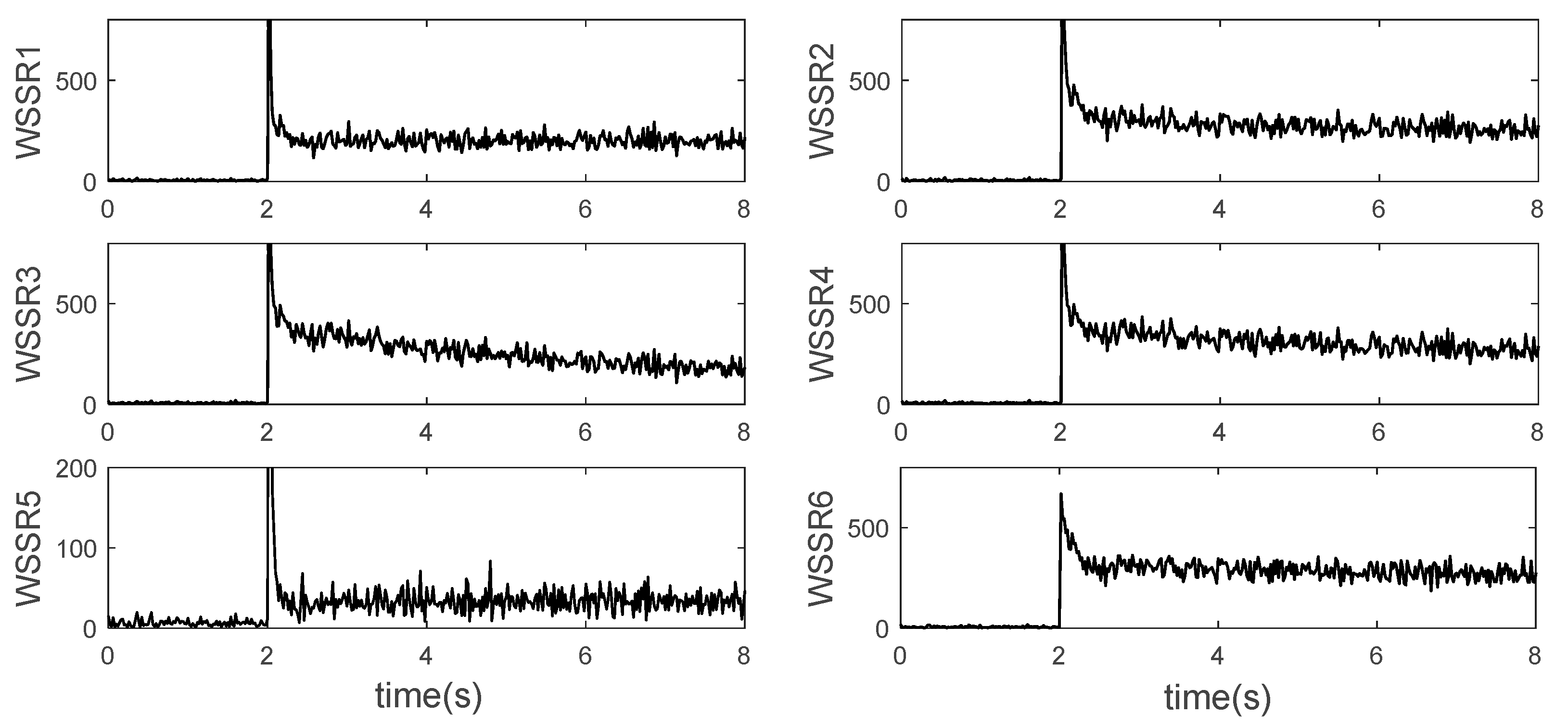
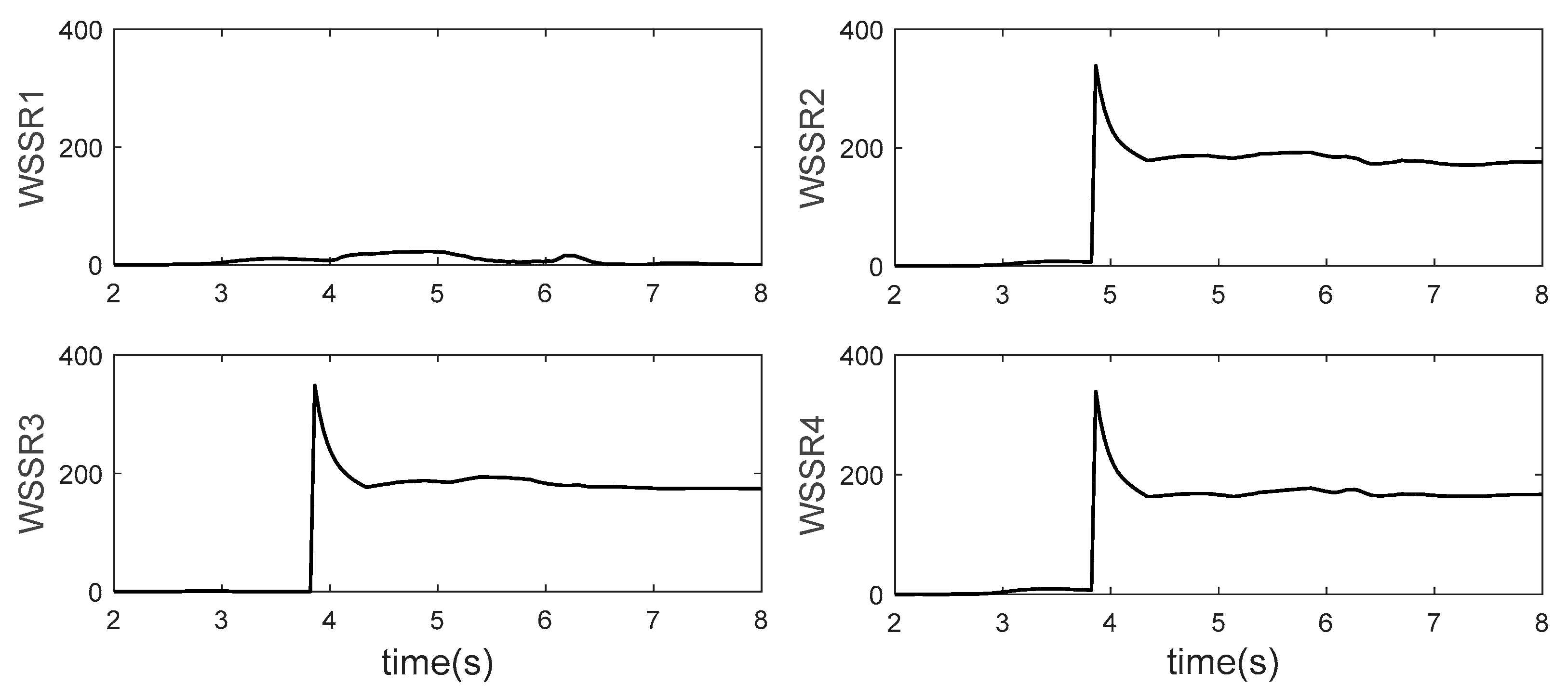
3. Sensor Fault Diagnosis

In this section, the AEMM is combined with the Kalman filter bank to design a fault diagnosis scheme for single sensor and double sensors. In the case of the single sensor fault, filter banks are designed. Each filter isolates one of the sensors, and the output estimation is carried out by using the remaining sensor information. In the case of the two sensor faults, they are grouped and the single-sensor diagnosis mode is adopted.

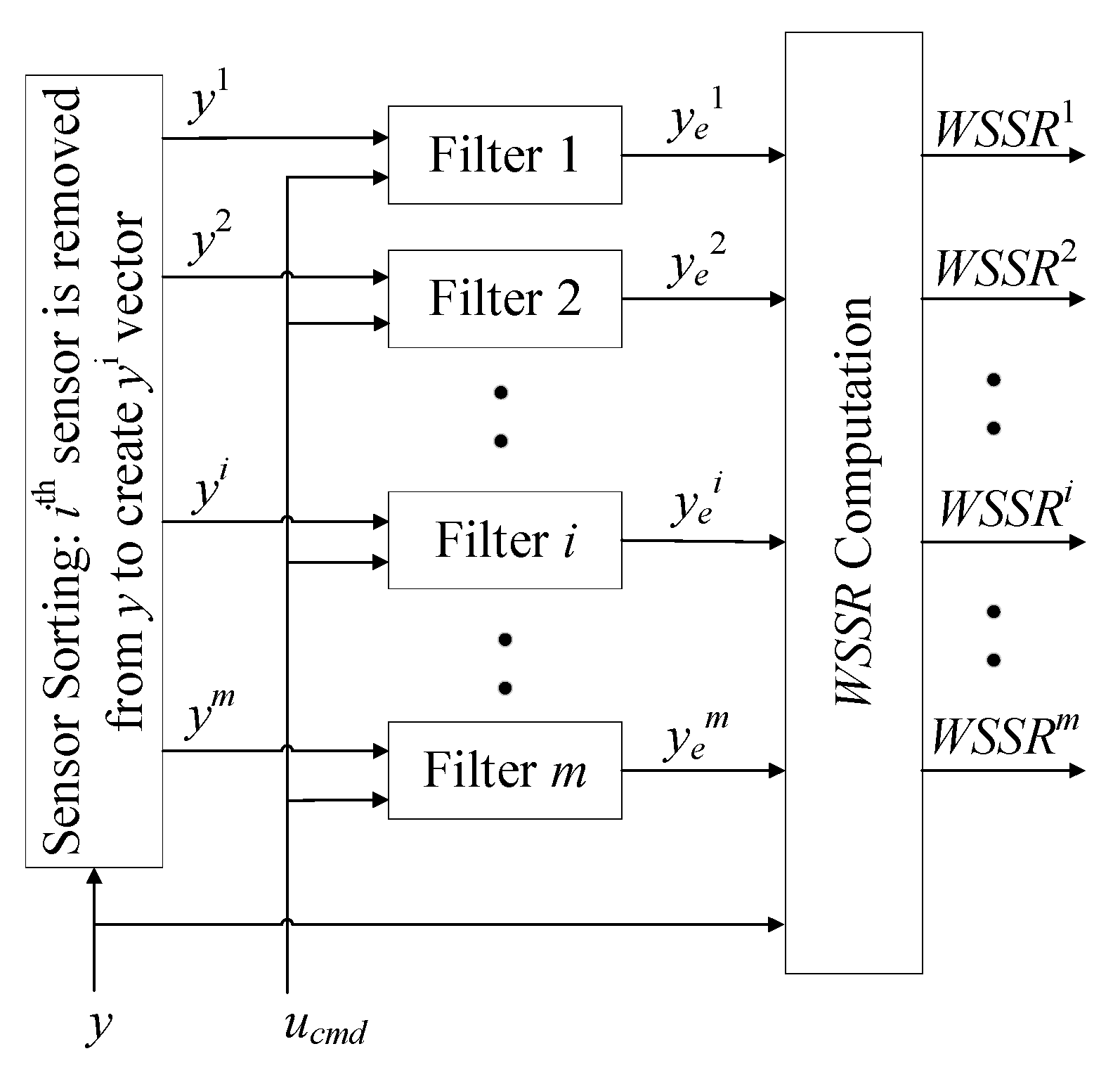
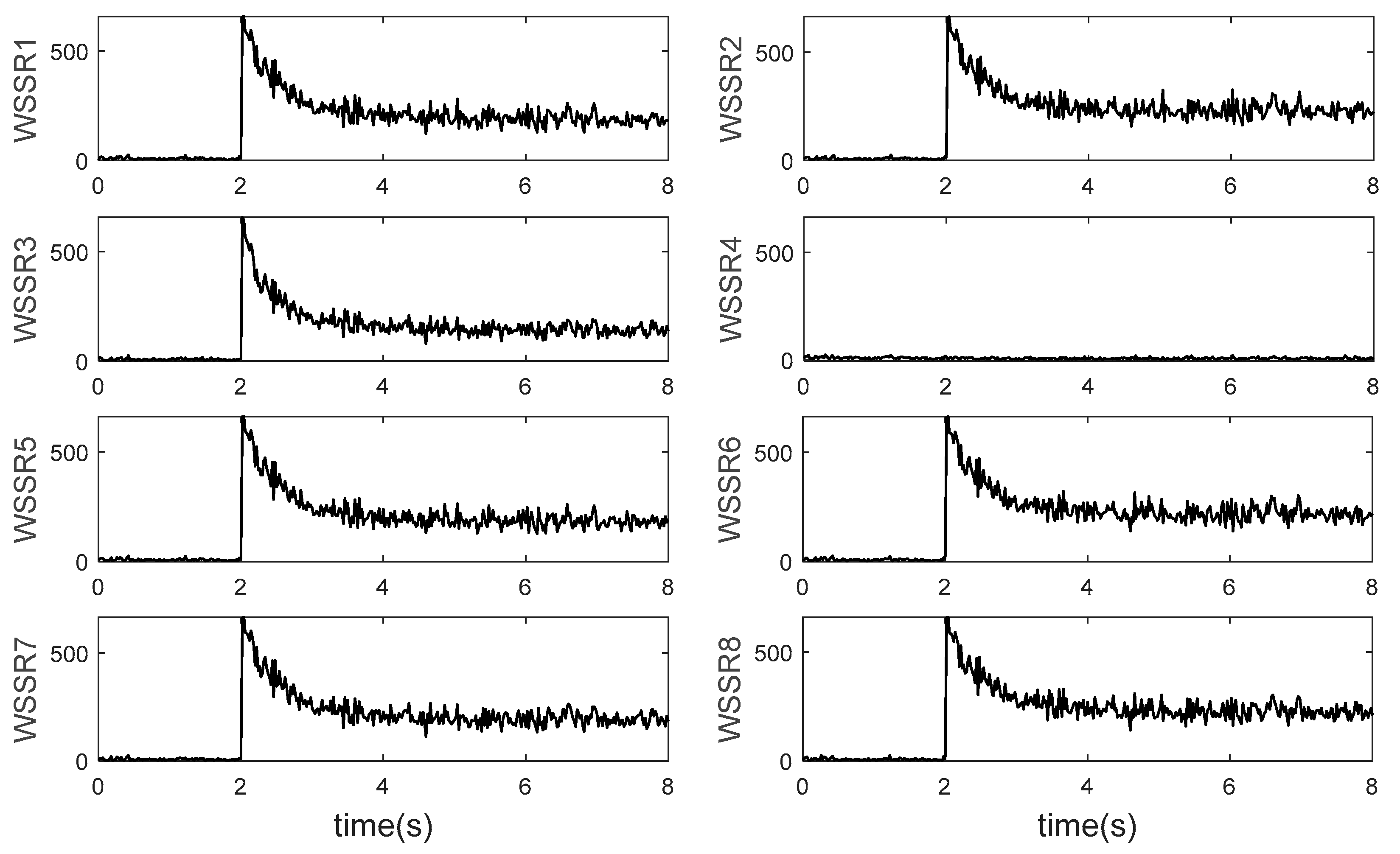
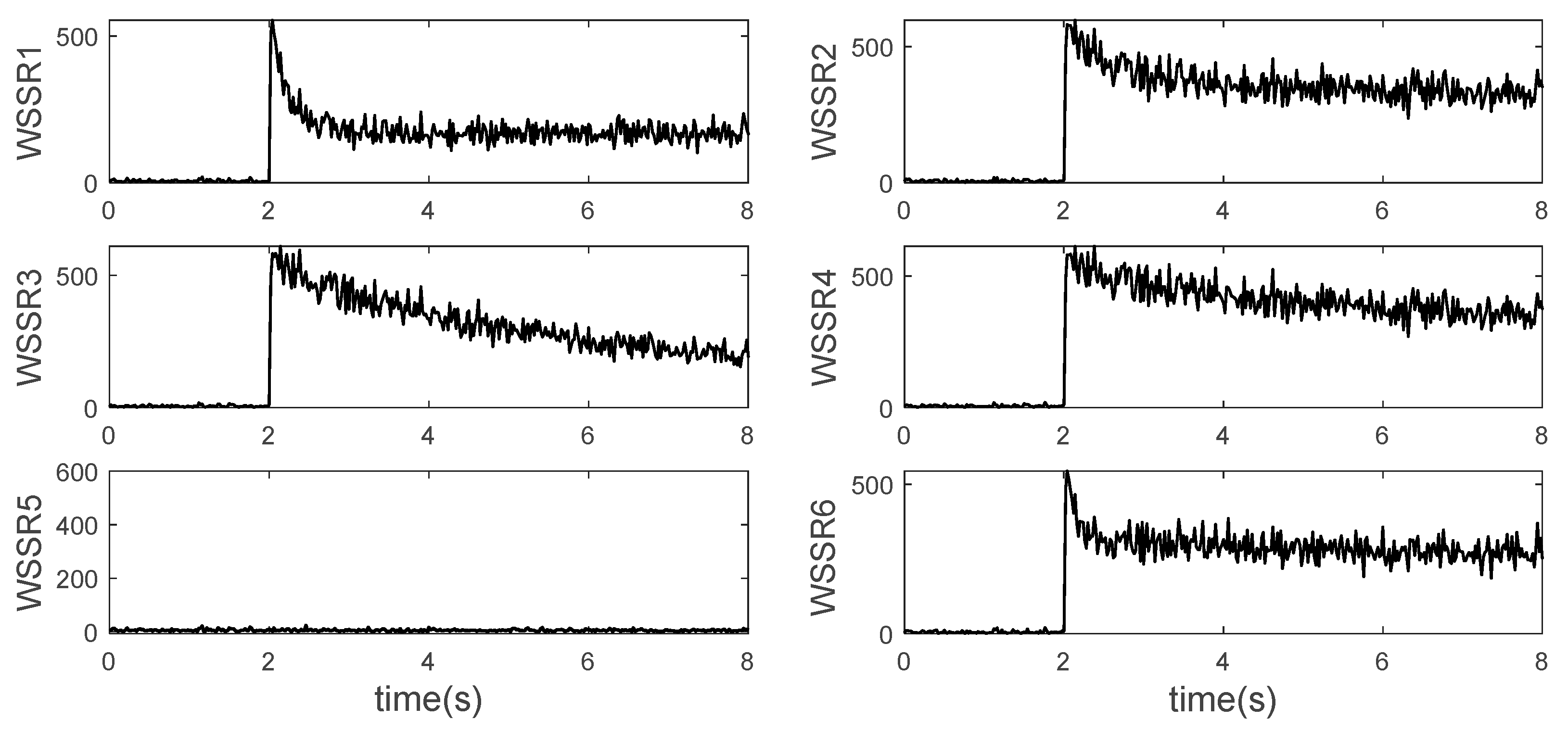
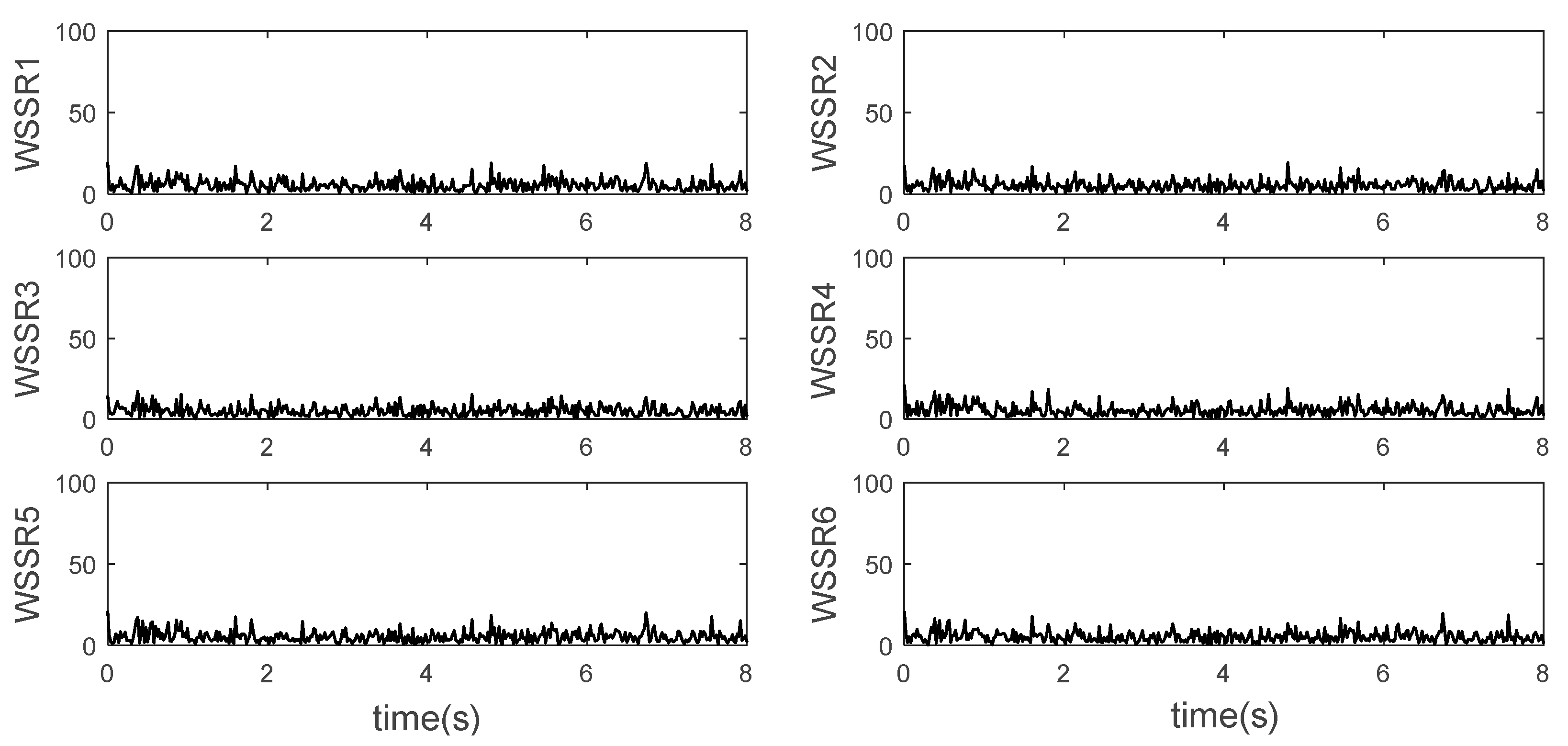
3.1. Single Sensor Fault

Assuming that m measurable parameters are used to estimate engine performance, m Kalman filters are designed accordingly. Each filter isolates the measured value of one of the sensors, and the remaining ( m 1 ) measured values are used for state/output estimation. The structure is shown in Figure 7. Take the ith Kalman filter as an example. Its input contains the remaining ( m 1 ) measurement values except for the ith sensor. After the failure of the ith sensor, the estimated values of the other filters are deviated from the actual measured values due to the access of the fault sensor signal. When the deviation of all the measured values is added up in a certain way, a relatively significant change can be obtained, and the faulty sensor can be identified. Moreover, since the ith filter is not connected to the fault sensor, the error between its estimated value and the actual measured value is small so that it can be used for fault signal reconstruction. The Kalman filter for the ith sensor is:
x ^ ˙ h ^ ˙ = A a u g x ^ x e α h ^ + K i y i y ^ i y ^ i y e i α = C a u g i x ^ x e α h ^
where y i is the subset of measurement parameters excluding the ith sensor, matrix C a u g i is the submatrix of matrix C a u g after removing the ith row, and K is the gain of the filter.
Define the residual between the filter input y i and the optimal output estimate y ^ i :
e i = y i y ^ i
when the sensor is fault-free and the filtering tends to be stable, the residual should obey the multi-dimensional standard normal distribution. However, when a fault occurs, the residual error does not possess this property, and its expectation is often not zero. Define the following variables:
WSSR i = W r i e i T σ i 2 1 e i
where WSSR is the weighted sum of squared residual. When there is no fault, WSSR obeys the χ 2 -distribution of ( m 1 ) degrees of freedom. W r i is the weight, and it can adjust the output of the filter. Its value will affect the diagnostic effect, resulting in misdiagnosis and missed diagnosis.
Select sensor measurement parameters as y = ( n l , n h , P t 3 , T t 3 , P t 21 , T t 21 , P t 6 , T t 6 ) . Compared with AEMM established previously, the four additional sensors are the total pressure and temperature at the fan outlet and the total pressure and temperature at the mixing chamber inlet. State quantity and health parameters remain unchanged. The noise matrices Q and R are reselected, and 8 Kalman filters are designed. The input of each filter is another 7 measured values. Set the efficiency of high-pressure turbine components to degrade by 2%, and obtain the steady-state deviations of 8 sensors under normal conditions: Δ n l = 1.98 % , Δ n h = 1.93 % , Δ P t 3 = 52.84   Kpa , Δ T t 3 = 10.0   K , Δ P t 21 = 0.28   Kpa , Δ T t 21 = 2.35   K , Δ P t 6 = 2.96   Kpa , Δ T t 6 = 21.18   K . At 2 s, a certain bias signal is injected into the outlet temperature sensor of the high-pressure compressor ( T 3 ). As can be seen from Figure 8, except for the fourth filter, the WSSR value of all the other filters underwent drastic abrupt changes and then gradually approached a stable value, while the WSSR value of the fourth filter remained at a low level. Therefore, it can be determined that the fourth sensor, the temperature sensor T t 3 , has failed. Then, a drift fault of 1 K/s is injected into the sensor. As can be seen from Figure 9, the WSSR of the other filters also drifts, while only the fourth filter remains unchanged. Therefore, the designed Kalman filter bank can diagnose all kinds of single sensor faults effectively.
Subsequently, this filter is used to re-estimate the degradation, and the result is shown in Figure 10, which is in line with the actual situation. Finally, the actual degradation is brought into the on-board AEMM to reconstruct the fault sensor signal, as shown in Figure 11, where the short red line is the fault sensor signal, and the solid black line is the corresponding sensor signal reconstructed from the on-board model.

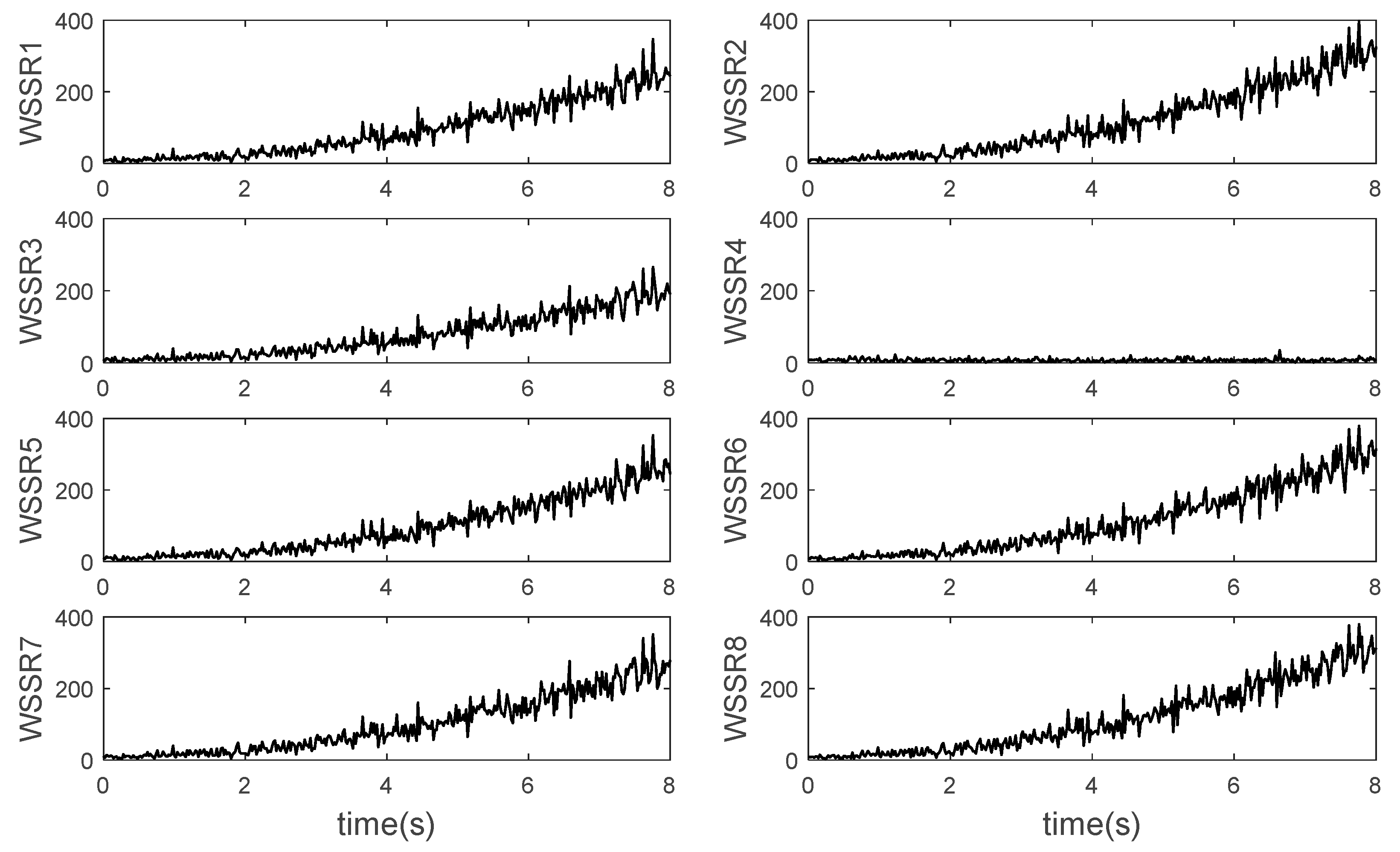
3.2. Dual Sensor Faults

Although the probability of simultaneous failure of two or more sensors is relatively low, due to the high-reliability requirements of engine control and fault diagnosis system, on the basis of being able to diagnose a single fault accurately, this section further studies the fault diagnosis and signal reconstruction of two sensors.
When the dual-sensor fault occurs, the Kalman filter design scheme that isolates one of the sensors mentioned above will not work because all the filters use the fault information. The output residual will make the WSSR of all the filters change. In this case, a conservative but effective scheme is to isolate the two sensors, but the number of Kalman filters required will increase as the number of combinations. So, when there are more sensors, the idea of grouping sensors can be used to design. For example, there are 2 N sensors, which are divided into groups A and B. Each group has N sensors. Kalman filter banks are independently designed for these two groups to carry out the single fault diagnosis. If both sensor faults occur in one group, the WSSR values of the filters in this group will deviate from the normal values, while the other group will keep low values. In this case, the signals in this group can be completely abandoned, and the optimal state estimation and signal reconstruction can be carried out with another group of filters. If sensor faults occur in both groups A and B, only one filter will remain low in both groups. The two fault sensors can be diagnosed and isolated at this time, and the remaining sensors can be used for optimal state estimation and signal reconstruction. Figure 12, Figure 13, Figure 14 and Figure 15 are the results of adopting this scheme. Group A contains the signals as y A = ( n l , n h , P t 3 , T t 3 , P t 21 , T t 21 ) while y B = ( P t 3 , T t 3 , P t 21 , T t 21 , P t 6 , T t 6 ) . Firstly, the fault sensors are set as the high spool speed sensor ( N h ) and the total pressure sensor at the inlet of the mixing chamber ( P t 6 ). As shown in Figure 12 and Figure 13, group A and group B each have a filter with a low WSSR value so that the fault sensor can be easily diagnosed. Secondly, the fault sensors are set as the total pressure sensor ( P t 6 ) and temperature sensor at the inlet of the mixing chamber ( T t 6 ). As shown in Figure 14 and Figure 15, it can be seen that the WSSR of all the filters in Group A remains low, while all the filters in Group B are offset. Therefore, it is judged that both sensor faults occur in Group B, and all sensors in Group A are normal. The methods for optimal state estimation and signal reconstruction using normal sensors are similar to those in the previous section and will not be repeated here.

4. Optimization Design of Acceleration Control Plan

4.1. Optimization Scheme of Control Plan Based on Target Shooting Method

In the 1980s, H.G.Bock proposed the idea of a direct multiple target shooting method, whose essence is to transform the optimal control problem into a parameter optimization problem [16,17]. Consider the following optimal control problem:
x ˙ t = f x t , u t , t .
The variation range of control variables and state variables is constrained as:
l 1 u t h 1 l 2 x t h 2 .
For initial state and terminal state, there are the following boundary conditions:
x ( 0 ) = x 0 x ( T ) = x T .
The optimal performance index is:
J = 0 T L x t , u t , t d t .
Terminal time T can be fixed or free. For the case where T is free, a new time variable τ 0 , 1 can be introduced. Let T be a variable parameter in a range and define t = T τ , d t d τ = T and d T d τ = 0 . At the same time, the augmented state variable x l + 1 and state equation are introduced:
x ˙ l + 1 = T L x τ , u τ , T τ , x l + 1 0 = 0 .
Thus, the above optimal trajectory problem is equivalent to the following Mayer problem [18] with fixed terminal time.
min f 1 x l + 1 1 , T .
The Equation of state of the system is as follows:
x ˙ = T f x τ , u τ , T τ = F x τ , u τ , T , τ .
The starting and ending constraints become:
x ( 0 ) = x 0 x ( 1 ) = x f .
Control variables, state variables, and process time constraints are shown in the following Equation:
L 1 u τ H 1 L 2 x τ H 2 . L 3 T H 3
Next, the Mayer problem can be solved by using a direct multiple target shooting method. The basic idea of the target shooting method is to transform the infinite dimensional problem into a finite dimension problem. The optimization process is divided into several intervals, and the design values of control variables and state variables are given in the interval nodes. In this way, the constraints on the whole process state and control variables can be transformed into constraints on these design values, and the performance indicators can also be transformed into functions of the design values. The following matching conditions should be considered: Set the change rule of the control quantity in each interval. It can be in the form of a constant value or polynomial. Then, the state variables at the end of each interval can be obtained from the guess value of the state variables at the beginning of the interval and the system state equation as shown in Equation (22). This value needs to be equal to the estimated value of the state here, which will be met by continuously revising the design value through the optimization algorithm. The specific steps of the target shooting method are as follows:
(1)
Divide the fixed time interval [0, 1] into m equal parts to get the node: τ i = i m , where i = 0 , 1 , , m .
(2)
Parameterize the control quantity. Introduce a set of vectors P i R q where i = 0 , 1 , , m and define:
u τ = u i P 0 , P i , , P m ,   τ τ i , τ i + 1 ,
where u i τ can be a constant value or some interpolation function.
(3)
Set up the initial value problem. A set of vectors S i R n is selected as an estimate of the state variables x i τ i at the node τ i . Then we have m initial value problems (IVP):
x ˙ i S i , u i , T , τ = F x i S i , u i , T , τ , u i τ , T , τ τ i , τ i + 1 ,
where the initial value is:
x i S i , u i , T , τ i = S i , i = 0 , 1 , , m 1 .
(4)
Constituting Nonlinear Programming (NLP). The optimization objective is:
min f 1 S m * , T ,
where S m * is the estimate of x l + 1 1 . The endpoints of each interval meet the matching conditions:
x S i , u i , T , τ i S i + 1 = 0 ,   i = 0 , 1 , , m 1 .
The starting and terminal states meet the boundary conditions:
S 0 = x 0 S m = x T .
Constraints on state quantity, control quantity and terminal time in the process are transformed into constraints on parameters at the end of the interval:
l 1 P i h 1 l 2 S i h 2 ,   i = 0 , 1 , , m l 3 T h 3 .
Finally, the Mayer optimization problem is transformed into a general NLP problem as shown in the following Equation.
min F 1 y F 2 y = 0 , F 3 y 0
where F 1 , F 2 and F 3 respectively represent the objective, equality constraint and inequality constraint function, and the optimization variable y is:
y = S 0 T , S 1 T , , S m T , P 0 T , P 1 T , , P m T , T T .
For the solution of the NLP problem, any NLP algorithm can be used, such as sequential quadratic programming, active set, interior point method, etc. In this paper, the Quasi-Newton method is used. The optimization variables are iteratively updated by the following formula:
y k + 1 = y k + t k Δ y k ,   t k t min , t max ,
where the increment Δ y k is determined by the Kuhn-Tucker condition of the quadratic approximation problem below:
min 1 2 Δ y T B k Δ y + F 1 k Δ y F 2 k + F 2 k Δ y = 0 F 3 k + F 3 k Δ y 0 ,
where F i k and F i k ( i = 1 , 2 , 3 ) are the values and gradients of the function at y k , and B k is the approximation of the Hessian matrix ( y 2 L ) of the following Lagrange equation:
L y , λ = F 1 y λ 1 T F 2 y λ 2 T F 3 y .
The above parameters can be updated by the following formula:
B k + 1 = B k + U B k , Δ y k , γ k γ k = L y k + 1 , λ 1 k , λ 2 k L y k , λ 1 k , λ 2 k ,
where U B k , Δ y k , γ k represents some correction method. The more commonly used is BFGS correction.

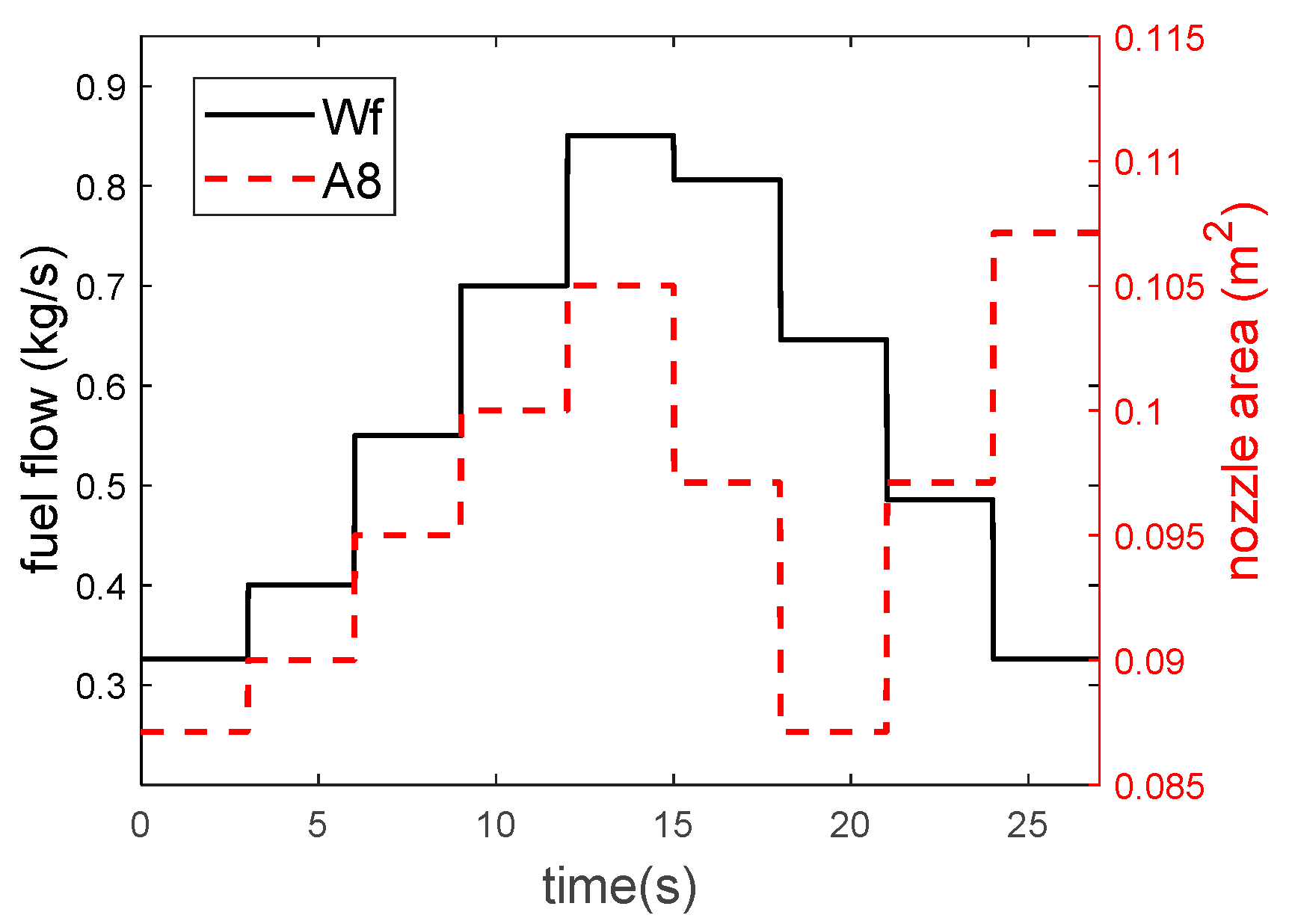
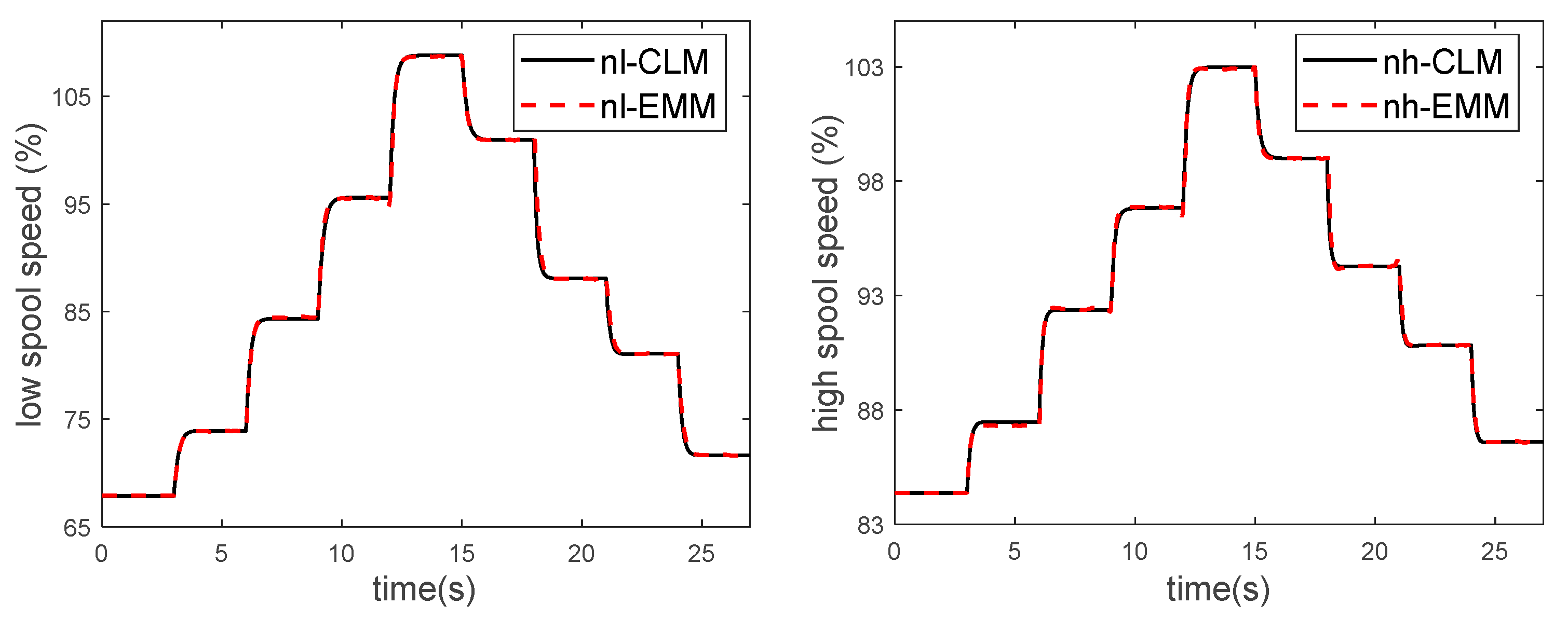
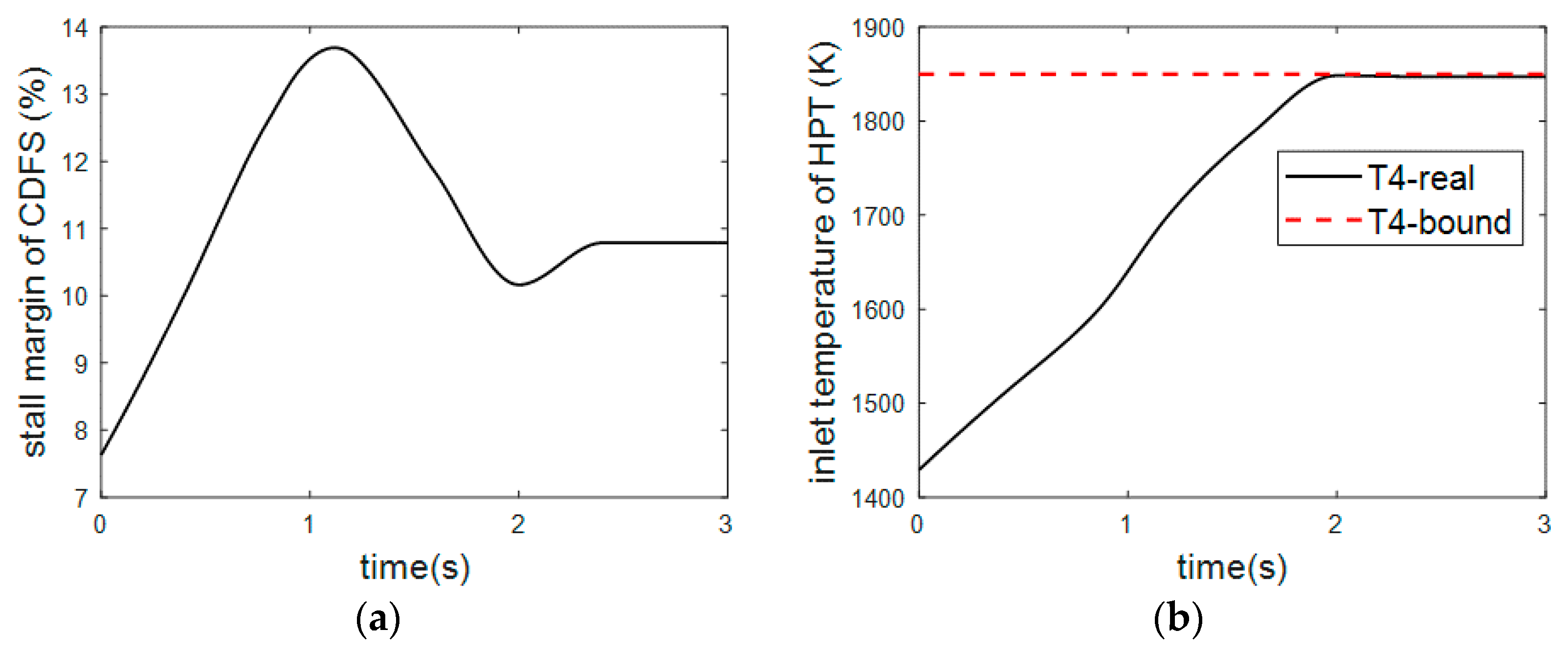
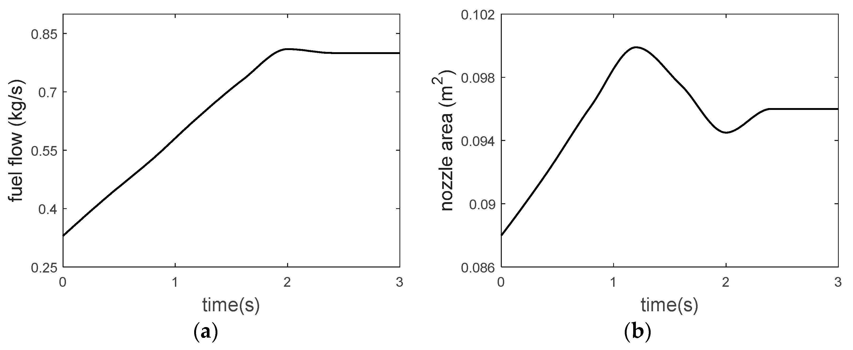
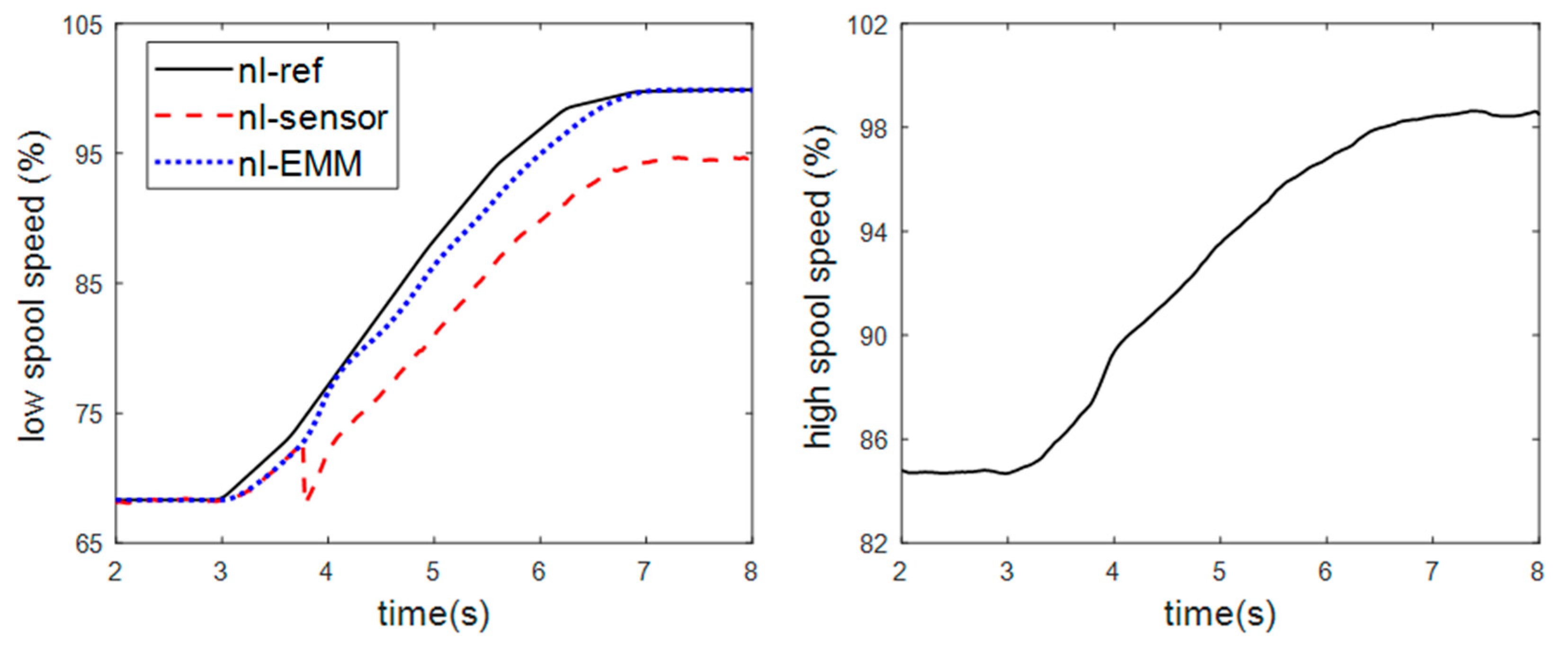
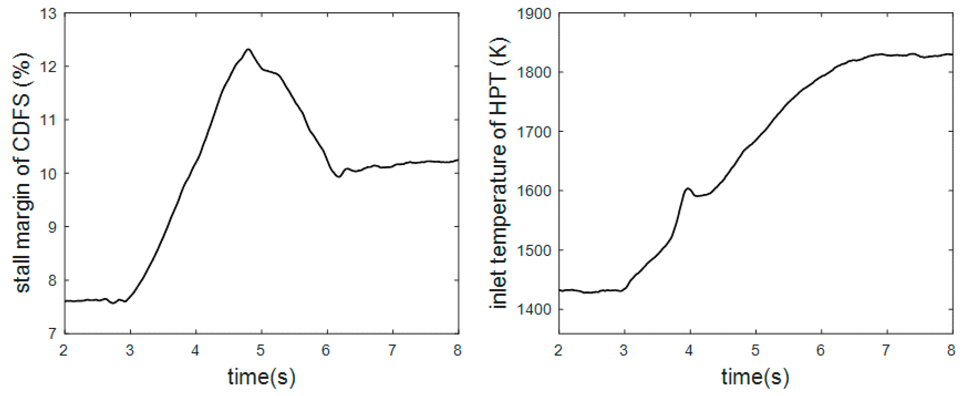
4.2. Accelerated Process Control Plan Design of VCE

Acceleration is the process of an engine from one thrust level to another. An important index to measure the performance of the acceleration process is acceleration time, which is mainly determined by the residual power of the engine. The main control variables of the acceleration process are the fuel flow and the nozzle area, among which the fuel quantity is the biggest factor affecting the engine acceleration performance. Increasing the fuel flow can increase the gas temperature in front of the turbine ( T t 4 ), thus increasing the power capacity of the turbine. However, it should be noted that T t 4 is limited by the strength of turbine blades and oil-rich flameout of the combustion chamber, and the sharp increase in fuel quantity will also cause engine speed to exceed limit and pose a certain threat to the mechanical load of the rotor. On the other hand, the acceleration process will lead to the decline of the compressor stability margin, so the compressor stability margin is often increased by opening the nozzle, deflating air, adjusting the guide vane of the compressor, etc.
Select the starting point of the accelerated process state x 0 and the control quantity u 0 :
x 0 : n l = 67.87 % , n h = 84.37 % u 0 : W f = 0.33   kg / s , A 8 = 0.088   m 2 .
Set the terminal state quantity x T and terminal control quantity u T :
x T : n l = 99.90 % , n h = 98.50 % u T : W f = 0.80   kg / s , A 8 = 0.096   m 2 .
The constraints in the optimization process are as follows:
n h < 100 % n l < 100 % T t 4 < 1850   K SM CDFS > 5 % SM HPC > 5 % W f < 0.84   kg / s A 8 < 0.1   m 2 W ˙ f < 0.25   kg / s 2 A ˙ 8 < 0.01   m 2 / s ,
where the last two terms represent the limit on the rate of change of the control quantity. The optimization objective is the shortest acceleration time:
min J = 0 T d t .
The AEMM is used as the optimization model of the accelerated process. Then the problem is modified to apply it to the target shooting method. Divide acceleration process into m intervals and the optimization variables y = S 0 T , S 1 T , , S m T , P 0 T , P 1 T , , P m T , T T can be obtained. The starting and ending constraints can then be translated into the following equality constraints:
F 1 ( y ) 1 = S 0 x 0 S m x T = 0 .
In addition, the state quantity of the starting point and the end point of each subinterval should be guaranteed to match.
F 1 ( y ) 2 = x S i , u i , T S i + 1 = 0 ,   i = 0 , 1 , , m 1 .
These two expressions together form equality constraints F 1 ( y ) . Note that the fourth-order Runge-Kutta method is used here to calculate the state quantities at the end of each interval. In the process, the restrictions on the high and low spool speed, the gas temperature in front of the turbine, the surge margin, the change rate of the control quantity, etc. are also easily expressed in the form of F 2 ( y ) < 0 . For example, the limit on the rate of change of fuel flow can be written as:
F 2 ( y ) 1 = ( P i + 1 , W f P i , W f ) T m 0.3 < 0 ,   i = 0 , 1 , , m 1 ,
where P i , W f represents the parameterized results of fuel flow at each node. The optimization goal is transformed into:
min F 3 ( y ) = T .
At this point, the problem has been transformed into an NLP problem as shown in Equation (32).
Solve the above problems, and the results are shown in Figure 16, Figure 17 and Figure 18, where CDFS represents the core drive fan stage of VCE.
It can be seen that the low spool speed changes from 67.87% to 99.9%, and the high spool speed changes from 84.37% to 98.5%. The acceleration time is about 2.4 s. The acceleration process is fast and stable without overshoot, and no overshoot occurs. At the beginning of acceleration, the dominant limiting condition is the rate of change of the control quantity, while at the later stage of acceleration, the dominant limiting condition is A 8 and the upper limit of T 4 . On the whole, the proposed accelerated process control plan meets the expected objectives.

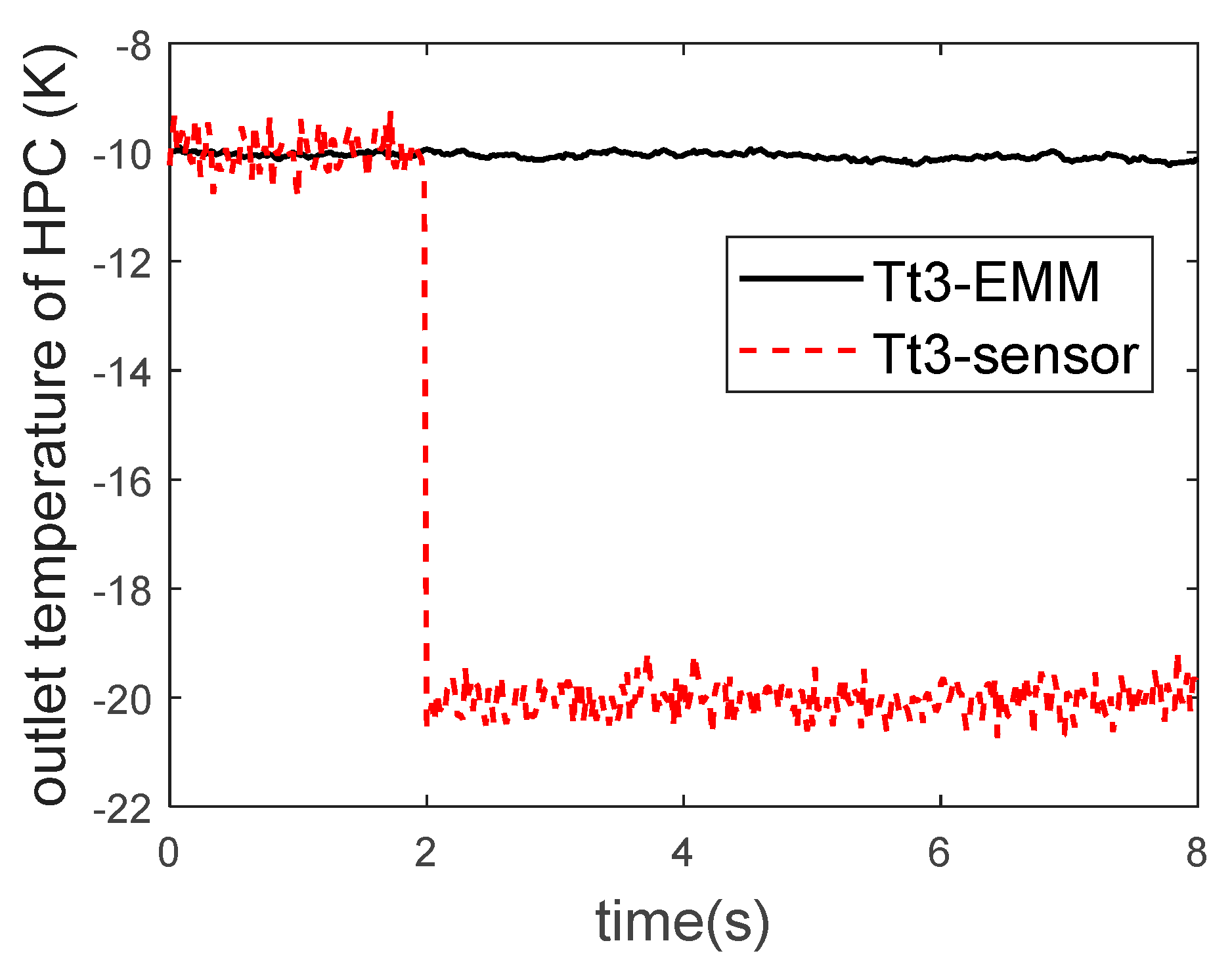
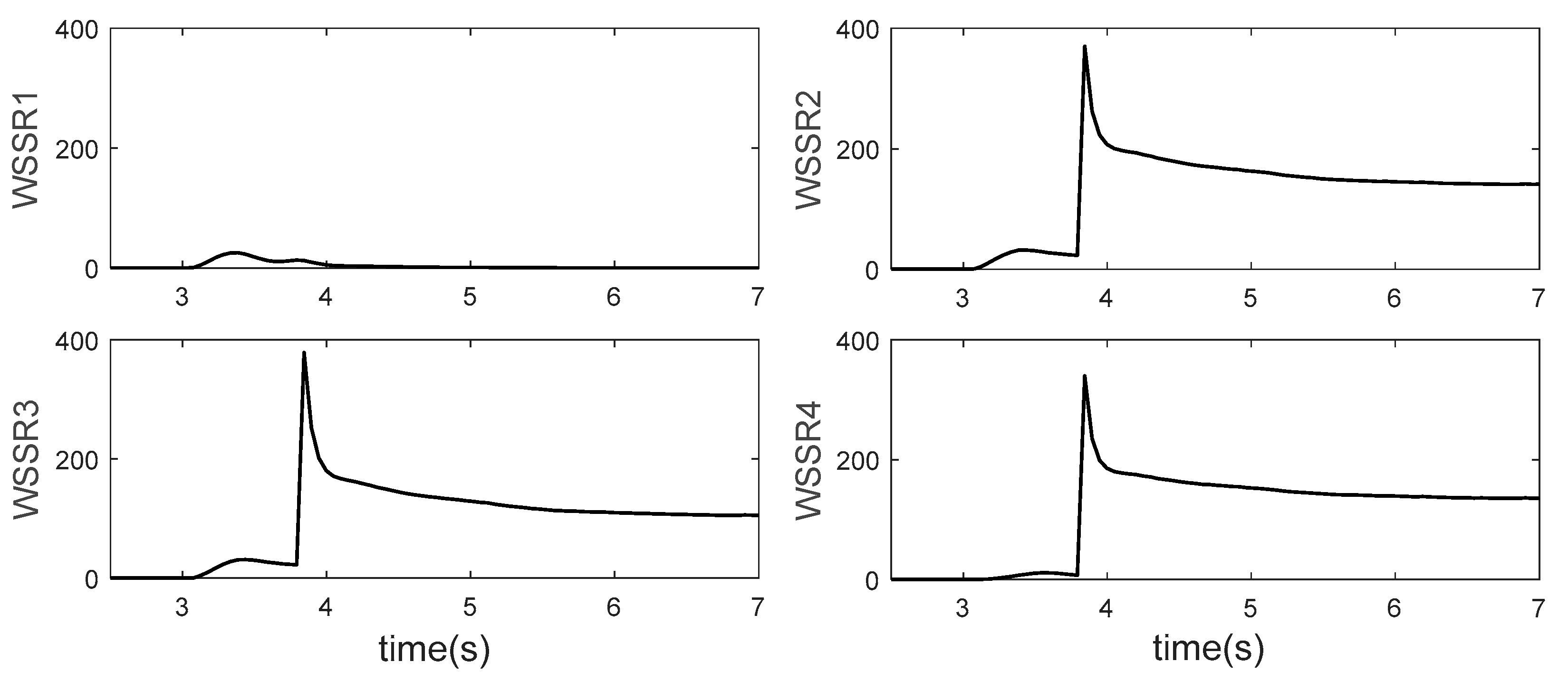
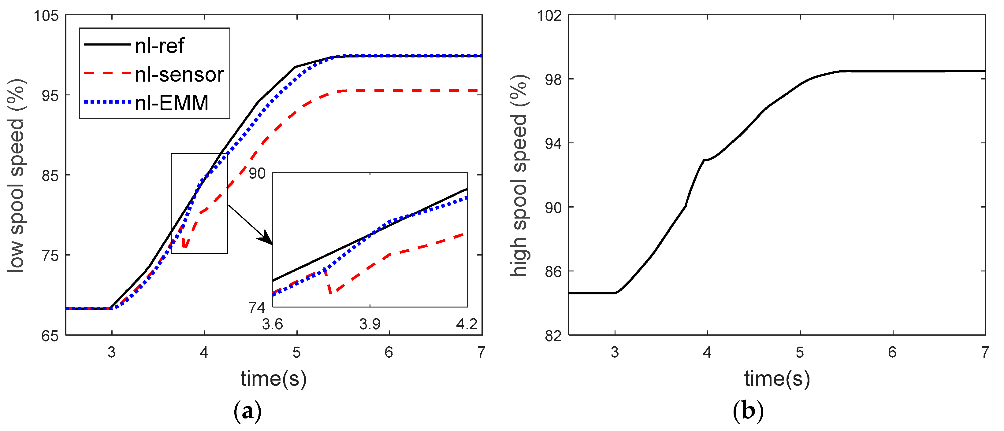
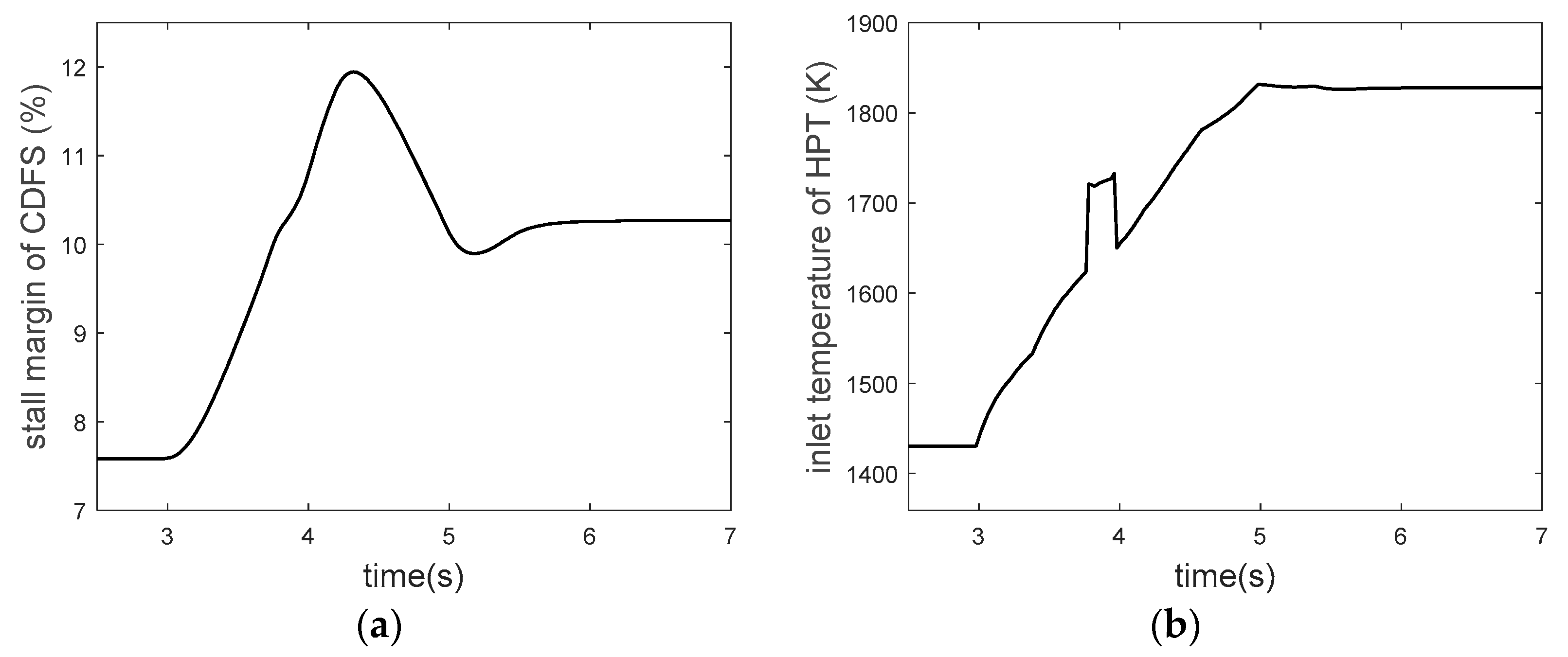
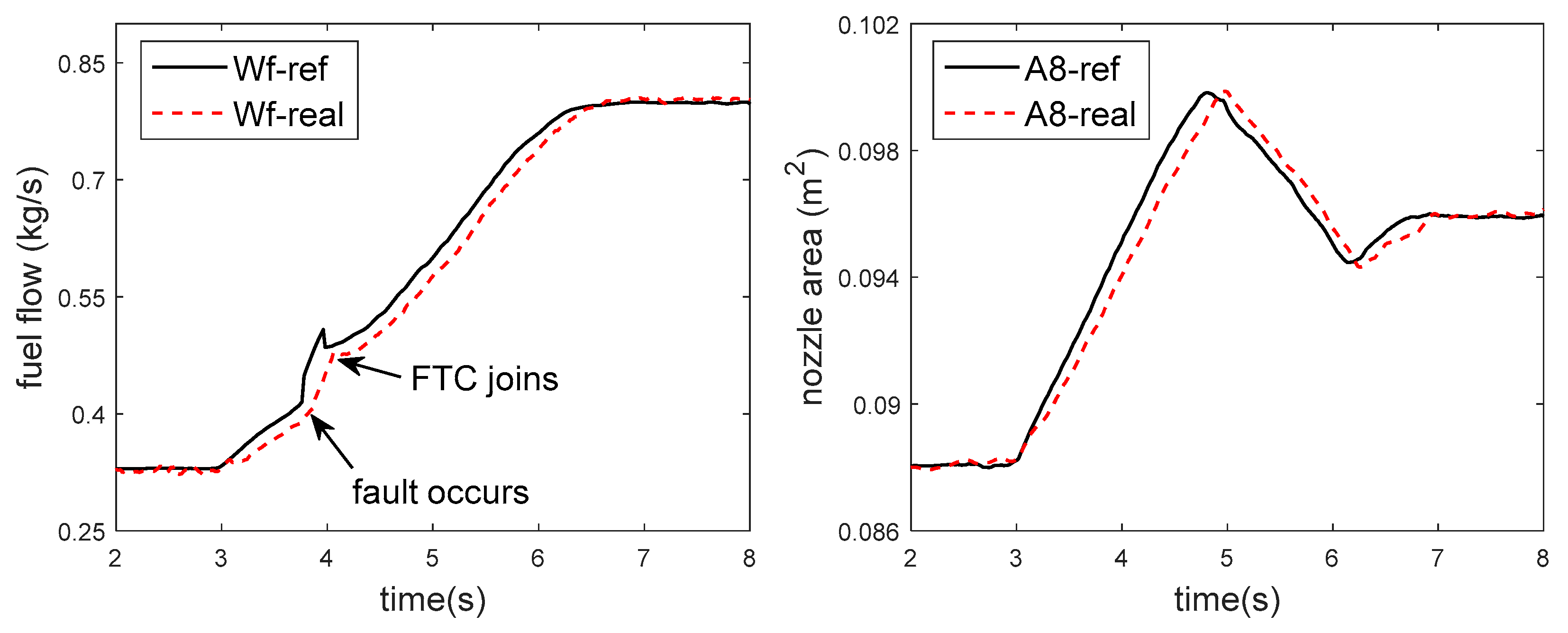
4.3. Sensor Fault Simulation

Use the variation rule of low spool speed and nozzle throat area optimized by target shooting method in 4.2 as control instructions for the acceleration process, and the acceleration control scheme of low spool speed closed-loop and nozzle throat area open-loop is adopted. The Kalman filter bank is designed by selecting sensors of low spool speed, high spool speed, high-pressure compressor outlet total pressure and total temperature, which constitute the sensor fault diagnosis module. Next, the sensor fault simulation in the acceleration process is carried out. The result is shown in Figure 19, Figure 20, Figure 21 and Figure 22.
At 3 s, the acceleration control begins. At about 3.8 s, 4% bias fault occurres in the low spool speed sensor, resulting in a large difference from the command speed. Therefore, the controller rapidly increases the amount of fuel to reduce the error between the two, as shown in Figure 22a. It can be seen from the changes of high spool speed and turbine front temperature that this adjustment leads to great changes in the actual engine state. From Figure 19, at 3.8 s the WSSR value of n h , P t 3 , T t 3 filters change greatly, and only the n l filter keeps a low value, so it is quickly determined that the low spool speed has been faulty. It is worth noting that the WSSR values of each filter also changes after 3 s, which is mainly caused by the difference between the on-board model and the real engine in the acceleration process. Compared with the change caused by sensor faults, the value is much smaller, so it does not affect the diagnosis. At about 4 s, the controller uses the analytical redundancy of low spool speed provided by the on-board model, and it can be seen that the engine states are restored. At about 5.4 s, the low spool speed output by the on-board model successfully keeps up with the control command, and the engine completes acceleration. In general, the scheme successfully achieves acceleration control under sensor faults. However, the sudden change of the control quantity caused by the sensor failure leads to the great change of the engine state, which is mainly because the actuation characteristics and small closed-loop control characteristics of the actuator are not considered in the digital simulation. Therefore, the hardware-in-the-loop test is used to further verify the results.

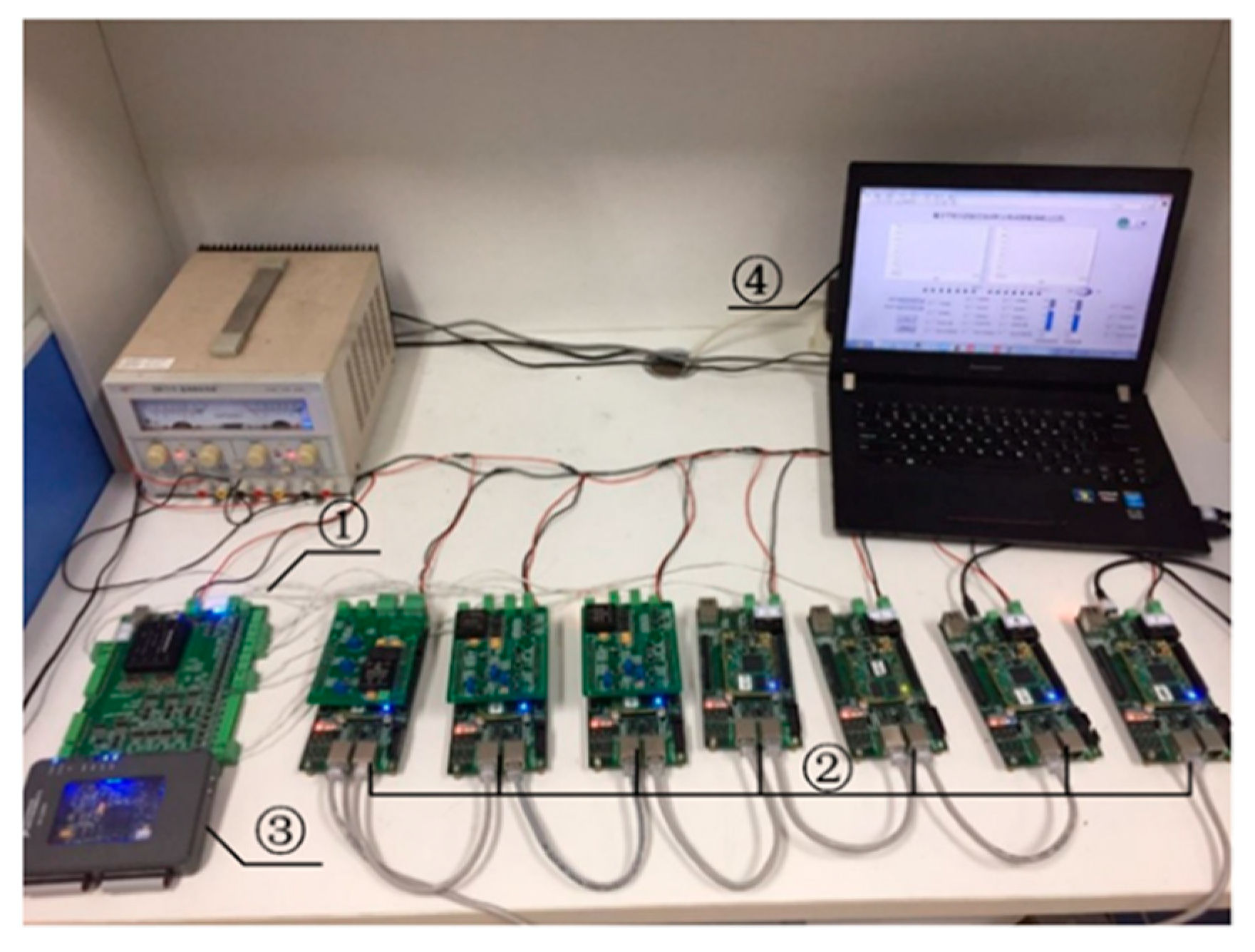
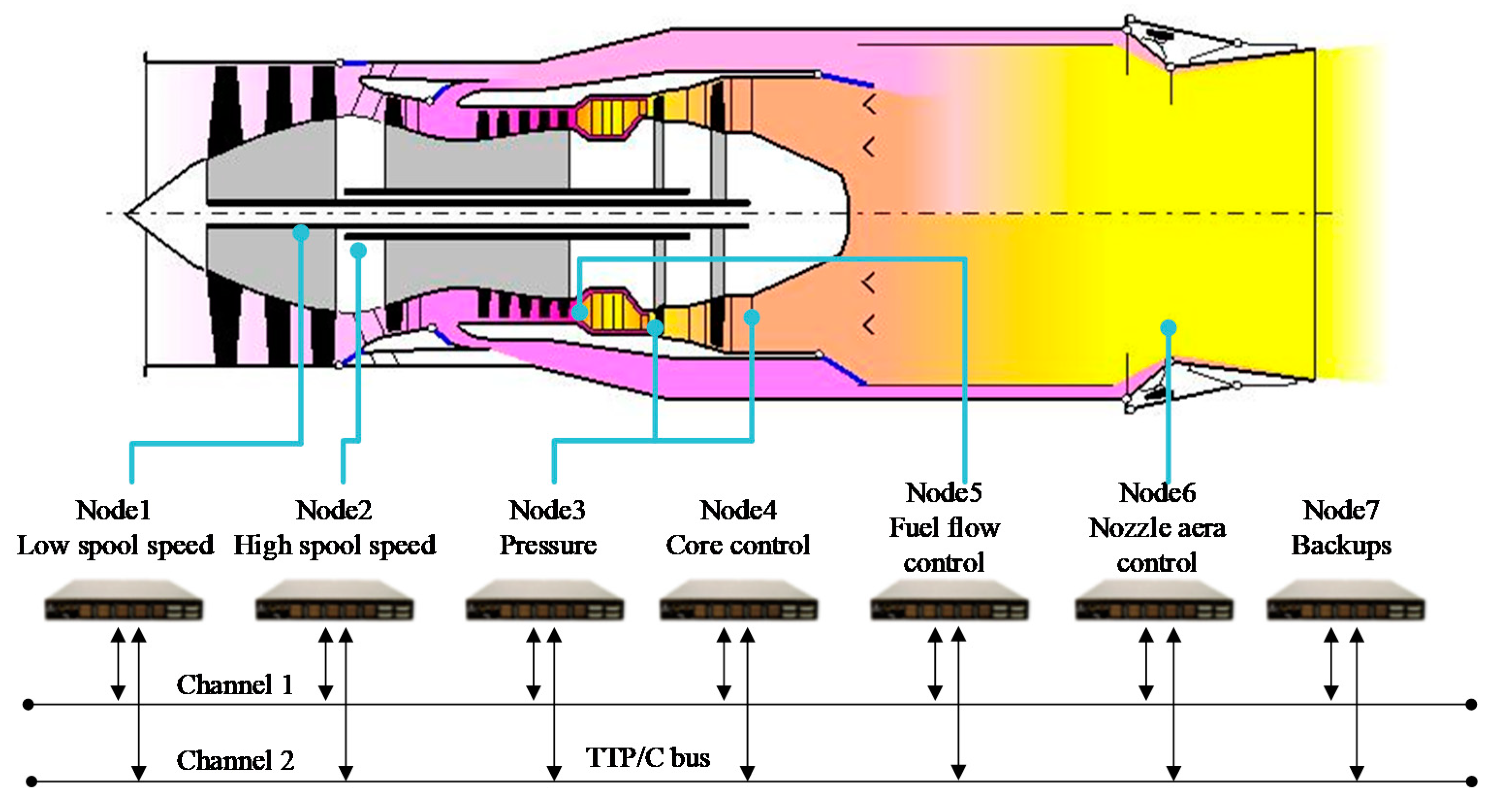
5. Hardware-in-the-Loop Simulation and Verification

The hardware-in-the-loop (HIL) test platform is shown in Figure 23 and Figure 24, which consists of an engine simulator, a distributed controller and a monitoring computer. The engine simulator includes NI myRIO and interface simulator. NI myRIO is responsible for the real-time operation of the engine model and simplified actuator model, and the interface simulator is responsible for simulating the signals of various sensors of the engine and collecting the current signals of actuator valves. The distributed controller comprises several intelligent nodes, including high and low spool speed acquisition node, pressure acquisition node, fuel flow control node, nozzle area control node, core control node and backup. Each intelligent node is an embedded system based on the ZYNQ development board and communicates with each other via the TTP/C bus. In addition to the tasks specified by TTP/C communication, each intelligent node also needs to complete the duties prescribed by the control system, which is conducted by two CPUs in the logical processing unit and the program processing unit in ZYNQ. The nodes are programmed and developed by Vivado’s integrated development environment and SDK software development suite. The monitoring computer is responsible for sending control instructions and monitoring the engine state, and is produced by LabVIEW. In terms of time schedule, the simulation step size of the engine simulator is 20 ms. In the distributed control system, the step size of the data acquisition node and the core control node is also 20 ms, while the step size of the actuator control node is 5 ms. Data transmission of each node on the TTP/C bus has a specified time sequence and is scheduled by a pre-planned Message Description List (MEDL).
The low spool speed, the high spool speed, the total pressure and the total temperature at the outlet of the high-pressure compressor are also selected for fault diagnosis and design. FTC results are shown in Figure 25, Figure 26, Figure 27 and Figure 28. At 3 s, the acceleration control starts. At this time, the speed of the engine and the speed of the on-board model is both good for tracking instructions. At about 3.8 s, a 5% bias occurs to the low spool speed sensor, as shown by the red dash in Figure 26. The controller rapidly increases the fuel flow control instruction, as shown in the solid black line in Figure 28. However, different from the result in 4.3, since the change rate of the actuator has reached the limit at this time, the actual fuel volume does not increase dramatically but maintains the maximum rate of increase. As shown in Figure 25, the low spool speed bias is quickly diagnosed by the Kalman filter, and the diagnosis effect is noticeable. At about 4 s, the reconstructed signal of the airborne model is switched for FTC and the fuel flow control instruction falls back. At 6.8 s, the reconstructed low spool speed signal keeps up with the control instruction and tends to a steady state, and the engine accelerates successfully. The fault diagnosis and signal reconstruction can be done within 0.2 s, and the whole FTC process can be carried out in less than 3 s. Parameters before and after the acceleration process are shown in Table 1. In general, the proposed scheme has good fault diagnosis ability and fault tolerance ability. The acceleration control under sensor fault is successfully realized, and the acceleration process does not cause a big change of engine state. Therefore, the validity of the FTC scheme proposed in this paper and its compatibility with the real-time embedded platform has been proved.

6. Conclusions

In this paper, an FTC scheme for the sensor fault in the transition process of VCE based on AEMM is proposed. The scheme adopts closed-loop control of speed and open-loop control of other control variables for transition control. To diagnose the sensor faults and study the control of acceleration process, a modeling study is first carried out. The fuel flow and the nozzle area are selected as the two scheduling variables to establish the EMM of VCE with multiple inputs and multiple outputs. Then the AEMM is obtained by introducing health parameters and Kalman filter. After that, the AEMM is combined with the Kalman filter bank to design a fault diagnosis scheme for the single sensor fault and double sensor faults. The simulation results of bias and drift fault cases show that the proposed scheme can accurately diagnose the fault sensors except when two fault sensors are grouped in the same group. But in either case, the scheme can accurately estimate the state and reconstruct the signal. Then, the target shooting method is used to optimize the engine acceleration control plan, and based on this, the fault simulation of the low spool speed sensor is carried out. Finally, a HIL simulation platform is built to verify the FTC method considering the actuation characteristics and other limitations of the actuator in the actual process. The results show that the fault sensor can be diagnosed and signal reconstruction can be carried out within 0.2 s by using the proposed scheme.
The method proposed in this paper can complete the FTC of sensor fault in a very short time, and is not too complicated, and has strong engineering feasibility and application value. At the same time, this method is also suitable for general turbofan engine fault-tolerant control. But there are still many areas that need to be further studied. For example, when two faulty sensors appear in the same group, only accurate signal reconstruction can be carried out, but the location of the faulty sensor cannot be diagnosed. And in addition to the acceleration process of the VCE, the FTC of the mode switching process should be paid more attention to. In this paper, only the fault-tolerant design of the sensor is carried out, and there may also be actuator fault, component fault and other forms. Therefore, the FTC problem of VCE needs more and more in-depth research.

Author Contributions

Conceptualization, L.L. and Y.Y.; methodology, L.L. and Y.Y.; soft-ware, X.Z.; validation, L.L., Y.Y. and X.Z.; formal analysis, T.Z.; investigation, S.W.; resources, T.Z.; data curation, L.L.; writing—original draft preparation, L.L.; writing—review and editing, S.W.; visualization, X.Z. All authors have read and agreed to the published version of the manuscript.

Funding

This research received no external funding.

Institutional Review Board Statement

Not applicable.

Informed Consent Statement

Not applicable.

Data Availability Statement

The data presented in this study are available on request from the corresponding author. The data are not publicly available due to the confidentiality of the data generated during the research process in this paper.

Conflicts of Interest

The funders had no role in the design of the study; in the collection, analyses, or interpretation of data; in the writing of the manuscript, or in the decision to publish the results.

References

  1. Hua, Y. Aero Engine Full Authority Digital Electronic Control System. In A Treatise on Electricity and Magnetism, 3rd ed.; Air China Media: Beijing, China, 2014. [Google Scholar]
  2. Baocheng, H. Application of simulation model of sensors to analysis fault of control system of turbojet engine. Propuls. Technol. 2001, 22, 364–367. [Google Scholar]
  3. Wallhagen, R.E.; Arpasi, D.J. Self-Teaching Digital-Computer Program for Fail-Operational Control of a Turbojet Engine in a Sea-Level Test Stand; No. NASA-TM-X-3043; National Aeronautics and Space Administatioin: Washington, DC, USA, 1974. [Google Scholar]
  4. Brown, H.; Vizzini, R.W. Analytical Redundancy Technology for Engine Reliability Improvement. SAE Aerosp. Technol. Conf. Expo. 1986, 95, 973–983. [Google Scholar] [CrossRef]
  5. Merrill, W.C.; DeLaat, J.C.; Bruton, W.M. Advanced detection, isolation, and accommodation of sensor failures—Real-time evaluation. J. Guid. Control Dyn. 1988, 11, 517–526. [Google Scholar] [CrossRef] [Green Version]
  6. Duyar, A.; Eldem, V.; Merrill, W.; Guo, T.-H. Fault detection and diagnosis in propulsion systems—A fault parameter estimation approach. J. Guid. Control Dyn. 1994, 17, 104–108. [Google Scholar] [CrossRef]
  7. Dewallef, P.; Léonard, O. Online validation of measurements on jet engines using automatic learning methods. In Proceedings of the 15th ISABE Conference, Bangalore, India, 3–7 September 2001; pp. 1–8. [Google Scholar]
  8. Mattern, D.L.; Jaw, L.C.; Guo, T.H.; Graham, R.; Mccoy, W. Using neural networks for sensor validation. In Proceedings of the 34th AIAA/ASME/SAE/ASEE Joint Propulsion Conference and Exhibit, Cleveland, OH, USA, 13–15 July 1998; p. 3547. [Google Scholar]
  9. Huang, X.-H. Sensor Fault Diagnosis and Reconstruction of Engine Control System Based on Autoassociative Neural Network. Chin. J. Aeronaut. 2004, 17, 23–27. [Google Scholar] [CrossRef] [Green Version]
  10. Yang, Q.; Wang, J. Multi-Level Wavelet Shannon Entropy-Based Method for Single-Sensor Fault Location. Entropy 2015, 17, 7101–7117. [Google Scholar] [CrossRef] [Green Version]
  11. Zhao, J.; Li, Y.; Qiu, T. A method for sensor fault diagnosis based on wavelet transform and neural network. Qinghua Daxue Xuebao/J. Tsinghua Univ. 2013, 53, 205–209. [Google Scholar]
  12. Chen, Y.S.; Jiang, S.D.; Liu, X.D.; Yang, J.L.; Wang, Q. Self-validating gas sensor fault diagnosis method based on EEMD sample entropy and SRC. Syst. Eng. Electron. 2016. [Google Scholar] [CrossRef]
  13. Liu, T.T.; Na, W.B.; He, N.; Li, M. Sensor Fault Detection Method Based on RBF Neural Network. Coal Mine Mach. 2017. [Google Scholar] [CrossRef]
  14. Liu, Y.; Chen, Q.; Liu, S.; Sheng, H. Intelligent Fault-Tolerant Control System Design and Semi-Physical Simulation Validation of Aero-Engine. IEEE Access 2020, 8, 217204–217212. [Google Scholar] [CrossRef]
  15. Yu, D.R.; Sui, Y.F. Expansion model based on equilibrium manifold for nonlinear system. J. Syst. Simul. 2006, 18, 2415–2418. [Google Scholar]
  16. Zhao, H.; Niu, J.; Jiang, Y.F.; Da-Ren, Y.U. Linear Modeling of Aero Engines Based on Balanced Manifold Model. J. Propuls. Technol. 2011, 32, 377–382. [Google Scholar]
  17. Lu, C.K. Research on Multivariable Control of Turbofan Engine Based on Equilibrium Manifold Model. Master’s Thesis, Harbin Institute of Technology, Harbin, China, 2019. [Google Scholar]
  18. Gou, X.Z.; Zhou, W.X.; Huang, J.Q. Component-level modeling technology for variable cycle engine. J. Aerosp. Power 2013, 28, 104–111. [Google Scholar]
Figure 1. Acceleration control scheme based on sensor fault-tolerance.
Applsci 12 02085 g001
Figure 2. Mapping of different scheduling variables.
Applsci 12 02085 g002
Figure 3. EMM vs CLM—input quantity.
Applsci 12 02085 g003
Figure 4. EMM vs CLM—output quantity.
Applsci 12 02085 g004
Figure 5. Estimation of degradation by AEMM.
Applsci 12 02085 g005
Figure 6. Estimation of measurements by AEMM.
Applsci 12 02085 g006
Figure 7. Schematic diagram of Kalman filter bank structure.
Applsci 12 02085 g007
Figure 8. WSSR value under single sensor bias fault.
Applsci 12 02085 g008
Figure 9. WSSR value under single sensor drift fault.
Applsci 12 02085 g009
Figure 10. Estimate of degradation after sensor troubleshooting.
Applsci 12 02085 g010
Figure 11. Signal reconstruction after sensor troubleshooting.
Applsci 12 02085 g011
Figure 12. Group A of dual-sensor faults grouping diagnosis—fault in different groups.
Applsci 12 02085 g012
Figure 13. Group B of dual-sensor faults grouping diagnosis—fault in different groups.
Applsci 12 02085 g013
Figure 14. Group A of dual-sensors fault grouping diagnosis—fault in the same group.
Applsci 12 02085 g014
Figure 15. Group B of dual-sensor faults grouping diagnosis—fault in the same group.
Applsci 12 02085 g015
Figure 16. Changing curve of speed during acceleration. (a) Low spool speed. (b) High spool speed.
Applsci 12 02085 g016
Figure 17. Changing curve of CDFS surge margin and turbine front temperature during acceleration. (a) CDFS surge margin. (b) Turbine inlet temperature.
Applsci 12 02085 g017
Figure 18. Changing curve of control quantity during acceleration. (a) Fuel flow. (b) Nozzle area.
Applsci 12 02085 g018
Figure 19. Sensor fault diagnosis results in acceleration FTC process.
Applsci 12 02085 g019
Figure 20. Changing curve of speed in acceleration FTC process. (a) Low spool speed. (b) High spool speed.
Applsci 12 02085 g020
Figure 21. Changing curve of CDFS surge margin and turbine front temperature in acceleration FTC process. (a) CDFS surge margin. (b) Turbine inlet temperature.
Applsci 12 02085 g021
Figure 22. Changing curve of control quantity in acceleration FTC process. (a) Fuel flow. (b) Nozzle area.
Applsci 12 02085 g022
Figure 23. Hardware-in-the-loop simulation platform. (1) Interface simulator (2) Distributed controller (3) NI myRIO (4) Monitoring computer.
Applsci 12 02085 g023
Figure 24. Schematic diagram of distributed control system structure.
Applsci 12 02085 g024
Figure 25. The sensor fault diagnosis results in the HIL test.
Applsci 12 02085 g025
Figure 26. Changing curve of speed in HIL test.
Applsci 12 02085 g026
Figure 27. Changing curve of CDFS surge margin and turbine front temperature in HIL test.
Applsci 12 02085 g027
Figure 28. Changing curve of control quantity in HIL test.
Applsci 12 02085 g028
Table 1. Parameters before and after the acceleration process.
VariableBefore the Acceleration ProcessAfter the Acceleration Process
Low spool speed (%)67.8799.9
High spool speed (%)84.3798.5
Stall margin of CDFS (%)7.6210.13
Inlet temperature of HPT (K)1435.251823.69
Fuel flow (kg/s)0.330.80
High spool speed (%)84.3798.5
Publisher’s Note: MDPI stays neutral with regard to jurisdictional claims in published maps and institutional affiliations.

