On the Relative Impact of Optimizers on Convolutional Neural Networks with Varying Depth and Width for Image Classification

Abstract

The continued increase in computing resources is one key factor that is allowing deep learning researchers to scale, design and train new and complex convolutional neural network (CNN) architectures in terms of varying width, depth, or both width and depth to improve performance for a variety of problems. The contributions of this study include an uncovering of how different optimization algorithms impact CNN architectural setups with variations in width, depth, and both width/depth. Specifically in this study, three different CNN architectural setups in combination with nine different optimization algorithms—namely SGD vanilla, with momentum, and with Nesterov momentum, RMSProp, ADAM, ADAGrad, ADADelta, ADAMax, and NADAM—are trained and evaluated using three publicly available benchmark image classification datasets. Through extensive experimentation, we analyze the output predictions of the different optimizers with the CNN architectures using accuracy, convergence speed, and loss function as performance metrics. Findings based on the overall results obtained across the three image classification datasets show that ADAM and NADAM achieved superior performances with wider and deeper/wider setups, respectively, while ADADelta was the worst performer, especially with the deeper CNN architectural setup.

1. Introduction

Neural network optimization algorithms continue to be a well-studied subject among researchers [1,2,3,4,5,6,7]. Training a deep neural network could largely be termed an optimization problem and is usually trained using stochastic gradient descent-based optimization algorithms. The main goals of researchers are to minimize the error function and accelerate convergence to an optimal global solution, with the overall objective of improving the model’s performance and its generalization ability. In this regard, optimizers are an important hyperparameter that affect the training performance of deep neural networks. Hence, it is important to choose the right optimizer for any given dataset problem that is being investigated, since the overall objective of neural network training is to minimize the prediction error by locating the global optimum on the loss surface. However, there is no consensus on this, so researchers are left with the task of experimenting with different optimization algorithms.

Several well-known optimization algorithms are used in training neural networks and can be broadly categorized into two: the classic stochastic gradient descent (SGD), which uses a static learning rate, and the adaptive stochastic learning rate such as ADAM and ADAGrad, which use adaptive learning rates. The learning rate is a key and central hyperparameter used by the optimizers for training neural networks and controls how fast a given model adapts to the problem it seeks to solve by helping the model to respond to the estimated error or loss each time the weights and biases values are updated. For instance, too large a learning rate could result in too fast a weights update, which may lead to instability in the training process and cause the model to converge prematurely to a suboptimal solution, whereas too small a learning rate may result in very tiny updates to the weights and a longer training process that could cause the model to be stuck in the local optima.

Researchers developed the adaptive learning rate optimizers as an improvement to the classic SGD because of the latter’s perceived slowness in arriving at an optimal solution and manually tuning the learning rate. However, one of the challenges still faced by these adaptive learning rate optimization algorithms is being trapped in local minima as against the desirable global minima [8], sometimes even exhibiting inferior performance in comparison to the classic SGD in some machine learning settings and problems [8], which has resulted in using a warm-up heuristic to mitigate these effects [9] and other ongoing improvements published in the literature. Among the adaptive learning rate optimizers, ADAM is the most popular among researchers due to its suitability in most problem cases. Because there is no consensus on the right optimizer to choose for a given task, as shown in a comparative study conducted in [10], researchers continue to work to address the issues with ADAM and other well-known optimization algorithms bordering around learning rate, stabilizing training, faster convergence, and improved generalization [6,11].

There have been two recent developments in optimization research for deep neural networks. First is a study that sought to develop an improved variant of ADAM called rADAM (rectified ADAM) [7]. The authors sought to address the underlying causes of sub-optimal convergence to local optima by rectifying the undesirable large variance of adaptive learning rate usually observed during the early stage of training in various neural network architectures and models. The root cause, they argue, is because of the limited training data at the initial training stage compared to the later stage. They advocated the use of a lower learning rate during the first few training epochs as a solution to alleviate the convergence problem.

Secondly, another recent study saw the development of the Lookahead optimization algorithm published by the authors in [6], which iteratively updates two weights, with the faster weights exploring or ‘looking ahead’, while the slower weights maintain the overall training stability of the neural network. The study was inspired by advances made in neural network loss surface research that allows a robust way to accelerate convergence and training stability All this is achieved with less hyperparameter tuning and minimal computational cost.

The backpropagation algorithm is key to fast learning in neural networks [12]. Backpropagation is a term that is used to compute the partial derivatives ∂C/∂w and ∂C/∂b of the cost function C, concerning any weight w and bias b in the network [13]. It gives insights into the overall behavior of the neural network in terms of how changing the weights and biases minimizes the cost function, which is determined by the gradients of the cost function. One of the factors that determine the stability and speed of network converge is the optimization algorithm; hence, it is worth examining how each optimizer’s update rule could make convergence faster, while at the same time maintaining high accuracy and low loss based on any given dataset-specific problem and the neural network architecture.

This paper extends the work in [14] in which the authors performed a comparative evaluation of the seven most commonly used first-order stochastic gradient-based optimization algorithms on a simple convolutional neural network architecture. In this current work, we go further to probe the impact of optimization algorithms on increasing CNN network sizes to understand their performance behavior. Accordingly, we pose the following questions: (1) How do different optimizers impact the learning performance of CNN architectures with variations in width, depth and width/depth on image classification problems? (2) Are there significant differences in the performance outputs?

Thus, we formulate a hypothesis for this study that given a non-convex problem, different optimization algorithms can find completely different solutions when initialized from the same point. We achieve this through an empirical study of different CNN architectures with varying network sizes to find out if we observe any discernable learning performance.

This leads us to the main contributions of the present paper, summarized as follows:

• We implemented three different wider, deeper, and wider/deeper simple CNN architectures.
• We conducted extensive experiments and analyzed the effects of nine different optimizers on increasing deepness, wideness, and deepness/wideness of the CNN architectures on three benchmark image classification datasets (Cats and Dogs, Natural Images, and Fashion MNIST).
• We provided insights into the effects of optimizers on CNN depth, width and depth/width architectures to inform optimal problem-specific CNN model design.

The remainder of the paper is organized in the following way: Section 2 presents a review of related works; Section 3 describes the different optimizers investigated in this study; and Section 4 presents the methodology of the study, including the experimental setup, summary of the dataset characteristics, and an overview of the CNN architectures studied. The experimental results and discussions are presented in Section 5. Section 6 concludes the paper. For clarity regarding the reminder of this paper, all acronyms adopted and used are provided in Table A1 of Appendix D.

2. Related Works

This section discusses briefly the fundamentals of CNN while analyzing the effects of optimizers on varying width and depth in deep neural networks and specifically on convolutional neural networks.

CNNs are deep learning algorithms that are widely used for image classification, image segmentation, and several other computer image tasks. They take in images and assign weights and biases to features of the input image. CNNs are popular because they require much lower pre-processing when compared to other image-classification algorithms. They have been employed in several image-processing tasks such as in detection of glaucoma [15,16], torsional evaluation of reinforced concrete beams [17], concrete crack detection [18], and other tasks.

Studies into how optimization algorithms impact the learning performance on varying depth and width in neural network models is a very active research area [19,20,21]. These studies aim to try to understand such behaviors both through theoretical and empirical perspectives across numerous application-specific problems [22]. In neural networks, model complexity has been achieved and analyzed by varying the network’s width and depth, or varying width while keeping depth constant, or vice versa [21,23]. However, this leads to an increasing number of parameters on one hand, but on the other hand achieves solutions that generalize well on training data, in contrast to the arguments in traditional statistical learning theory that increasing the number of parameters in machine-learning models will most likely overfit training data and therefore generalize poorly to unseen test data [24]. The double descent risk curve proposed by [20] sought to reconcile this apparent conflict in neural networks, where they observed that beyond the fitting threshold, the risk decreases as model complexity increases.

The authors [25] analyzed the bias-variance effect of deep CNNs and observed that as depth increases, bias decreases greater than the increase in variance, and suggested the possibility for deeper networks to have increased risk.

The authors [21] went further to critically analyze the effect of increasing depth on CNN test performance, specifically using ResNets and fully-convolutional networks model on CIFAR10 and the ImageNet32 dataset, while holding the network’s width constant. They observed that the test performance of the networks worsens when increasing network depth beyond a critical point, in contrast to increasing model complexity through width. They also suggested that double descent happens only through width and not through depth, and that deeper networks can have an increased risk of generalizing poorly to unseen data. They trained their models using ADAM, SGD and SGD with momentum optimizers.

In the work of [22] the authors studied the effects of depth and width on the learned internally hidden representations, aimed at finding characteristics of the block structure in the hidden representations with varying network capacity of wider or deeper neural network models. They show that block structure arises when the model capacity is large relative to the size of the training dataset. They observed that the features learned by different models outside the block structure are often similar across architectures with varying widths and depths, but the block structure is unique to each model. Upon analyzing the prediction outputs of the different architectures, they concluded that even when the overall accuracy is similar, wide and deep models exhibit distinctive error patterns and variations across classes. The study was carried out using a family of ResNet models with varying depths and widths, and trained on CIFAR-10, CIFAR-100 and ImageNet datasets using SGD with momentum.

Other works such as [26] studied the effect of depth on CNN models with two variations of depths, while the authors of [27] examined the role of depth in CNNs, and another study [28] studied optimization in deep CNNs where the authors observed that increasing depth increases representational power while increasing width smoothes the optimization landscape. A paper by [19] looked at the potential pitfall of adaptive gradient methods finding solutions that generalize worse than SGD despite having the same training loss, and argued against the increasing use of adaptive gradient methods, specifically ADAM, by the deep learning community in all scenarios. The authors of that paper also observed that adaptive learning rate methods often exhibit faster initial progress during training, but their learning performance quickly reaches a critical saturation point on the test set. This has led to some researchers advocating the use of both adaptive methods such as ADAM at the initial stages of training and switching to non-adaptive SGD at a later stage to improve generalization [29]. However, the works of [30] observed that with sufficiently tuned hyperparameters, adaptive methods would never underperform momentum or SGD, while [31] concludes that with sufficiently tuned hyperparameters, standard optimizers such as SGD and ADAM would never underperform state-of-art optimizers for large batch size settings. However, it all comes at the expense of higher computing costs. While all of these works acknowledged that optimizers do impact the performances of different neural network architectures across various theoretical and empirical settings, they did not provide an explicit connection on the effect that different optimizers have had on the increasing complexity of CNN architectures in terms of varying width, depth and width/depth, which is the focus of the current work.

Table 1 is a summary of the most relevant works referenced in this study in terms of the models, optimizers, image dataset used and their contributions.

Table 1. Summary of relevant works.

Study	Model	Optimizer	Image Dataset	Contribution
[20]	Fully connected CNN	SGD, momentum	CIFAR-10, MNIST, and SVHN	Double descent risk curve that reconciles the bias-variance tradeoff curve and observed behaviors of modern machine learning models
[21]	ResNet, CNN	ADAM, SGD, momentum	CIFAR10 and ImageNet32	Deep networks may have an increased risk of poor generalization on testing data sets
[22]	Family of ResNet	SGD momentum	CIFAR-10, CIFAR-100, Image Net	Deep and wide models may have similar overall accuracy, but they do exhibit distinctive error patterns and variations across different classes
[19]	Deep CNN, 2-layer-LSTM, 2-Layer LSTM with Feedforward, 3-Layer LSTM	SGD, Heavy-ball momentum, ADAGrad, RMSProp, and ADAM	CIFAR-10	Observed that adaptive learning rate methods often exhibit faster initial progress during training, but their learning performance quickly reaches a critical saturation point on the test set. Both SGD and ADAM performances could improve with hyperparameters tuning.
[30]	Simple 2-layer CNN, 3-layer CNN, ResNet-32/50 and VGG-16	SGD, momentum, Nesterov, RMSPROP, ADAM, and NADAM	Fashion MNIST, CIFAR-10/100, ImageNet	With sufficiently tuned hyperparameters, adaptive optimizers would always outperform momentum or SGD. Proves inclusion relationships between optimizers’ implementations.
[31]	ResNet-50	SGD momentum, Nesterov and ADAM	ImageNet	Discovered that sufficiently hyperparameter tuned standard optimizers would never underperform state-of-art optimizers (LARS and LAMB) for large batch sizes.

3. Optimization Techniques

Optimizer is an important hyperparameter needed for training deep learning models They are broadly categorized into two for non-convex optimization problems, namely, non-adaptive learning rate (classical SGD), and adaptive learning rate optimization algorithms [5,32]. Although there is also a second-order optimization algorithm for convex problems, the main difference between convex and non-convex optimization problems is that for convex optimization problems there is only one global optimum, with no notion of local optima, whereas the non-convex optimization problem has multiple local optima across the neural network loss surface, with only one global optimum [32]. The focus of this paper is on first-order optimization algorithms for non-convex problems. This is because non-convex optimization problems are the most prevalent in neural network research. The nature of the loss surface for non-convex problems determines the complexity and difficulty in locating the global optimum [33]. An optimizer is therefore used to reduce the cost function which is calculated by cross-entropy, while the loss function is used to calculate the error which is the metric that indicates the efficiency of the model.

A brief overview of the examined optimizers is described as follows:

• Non-adaptive SGD and its enhanced variants are based on the gradient descent approach. Gradient descent is a means to minimise an objective function f (x) parameterised by a model’s parameters x $\in$ ℝ, by updating the parameters in the opposite direction of the gradient of the objective function ${\nabla }_{x}f\left(x\right)$ with regard to the parameters reaching the local minimum which is determined by the learning rate [3]. SGD uses a single training dataset, one row after another, and then followed by iteration adjustment of weights for each row. Oscillation because of stochastic noise in SGD is one of its problems, resulting from updates not capturing curvature information and thereby slowing down SGD when loss surface curvature is high. Momentum is a technique, when applied to SGD, that dampens these oscillations [32,34]. This is achieved by accelerating the gradient descent towards reducing the objective function across iterations through tailoring the accumulated velocity vector towards that objective. Given an objective function f (x), momentum is defined as [9]:

  $$v_{t+1}=\mu v_t-\epsilon {\nabla }_{x}f\left(x_t\right)$$

  (1)

  $$\begin{array}{c}{x}_{t+1}=x_t+v_{t+1}\end{array}$$

  (2)

  where $\epsilon$ = learning rate; $\mu$ = momentum coefficient; and ${\nabla }_{x}f\left(x_t\right)$ = gradient at x_t; when $\epsilon >0$; $\mu ϵ \left[0, 1\right]$.

In SGD with momentum, the gradient-based velocity vector is first corrected/updated in the current position $x_t$, and then a big step is taken based on this new velocity vector value. In contrast, in SGD with Nesterov momentum, the first step is taken along the direction of the velocity and then correction and update to the velocity vector value is made based on the new location $x_t+\mu v_t\cong x_{t+1}$. Hence, Nesterov momentum is given (taking into account the new velocity vector update) as [9]:

$$\begin{array}{c}{v}_{t+1}=\mu v_t-\epsilon {\nabla }_{x}f\left(x_t+\mu v_t\right)\end{array}$$

(3)

$$\begin{array}{c}{x}_{t+1}=x_t+v_{t+1}\end{array}$$

(4)

• ADAGrad was designed as an improvement to the non-adaptive SGD optimization when the gradient vectors are sparse, particularly in the online learning setting [35]. Generally, with the overall objective of achieving faster convergence time [11], most of the adaptive learning rate techniques developed over the years are variants of ADAGrad, as they seek to address some inherent and notable weaknesses in ADAGrad, such as the rapid decrease in the learning rate in non-convex settings due to the accumulated squared gradient over time [11].
• RMSProp is a modification of ADAGrad to improve performance in non-convex situations. It is based on the idea that dividing the vector gradient by the root mean square for each weight improves learning [36].
• ADAM combines the strengths of RMSProp and SGD with momentum [37]. It uses the squared gradient method as in RSMProp for scaling the learning rate as well as the moving average of the gradient leveraging on momentum [37]. ADAM also combines the advantages of ADAGrad and RMSProp, and works well in settings with sparse gradients and online settings [35,36]. This is the reason why ADAM can perform well across numerous problem domains and datasets.
• ADADelta is a method developed to combat the issue with the accumulation of all past squared gradients in ADAGrad, which affects the learning rate by decreasing it towards zero and eventually terminating training. ADADelta is a remedy to prevent the continual decay of learning rates and to avoid the need to select the global learning rate manually [37,38].
• ADAMax is a variation of ADAM that uses the L-infinity ($L^{\infty })$ norm rule to update present and past gradients, resulting in stable behavior. Given a generalised $L^p$ norm-based update rule, the ADAM algorithm becomes numerically unstable in situations for norms with large $p$ values [37].
• NADAM is a combination of RMSProp and Nesterov momentum. It builds on the work of [36] by incorporating Nesterov momentum into ADAM, rather than using only momentum to estimate the exponential moving average of the gradient [39], and thus making NADAM an improved variant of ADAM.

A brief explanation of the optimizers update rule is provided in Table 2:

Table 2. A brief explanation of optimizer update rules.

Optimizer	Brief Explanation of the Update Rules
VSGD	Performs parameter update in the opposite direction of the objective function’s gradient. This is carried out for each training sample at once using the same learning rate.
SGDM	Very similar update rule to SGD but accelerates the optimizer in the current direction while reducing the occurrence of high oscillations.
SGDNM	Also has the same update rule as SGD but gives the accelerating optimizer a prenotion of where the next direction might be. Hence, helping the optimizer to know when to reduce its velocity.
ADAGrad	This optimizer uses different learning rates every time, for every parameter, using previously computed gradients. The optimizer removes the requirement of tuning the learning rates when training.
RMSProp	Similar to the update rule used in ADAGrad but divides the computed learning rate by the root mean square of the gradients. This reduces the rate at which the learning rate diminishes.
ADAM	The optimizer computes both the exponential decaying average of previous squared gradients (used in RMSProp) and the exponential decaying average of previous gradients (used in SGD with momentum). These computed values are applied to update the model’s parameters.
ADADelta	Similar to the update rule used in ADAGrad but uses a fixed size of past gradients instead of using all the past gradients to compute the relevant learning rate.
ADAMax	Similar to the ADAM update rule but introduces a value that relies on the max operation based on the proposal that the $L^{\infty }$ norm and the gradients converge to this value.
NADAM	The update rule combines RMSProp with Nesterov momentum (as used in the SGD with Nesterov momentum)

4. Materials and Methods

This section presents the experimental setup, summary, and characteristics of the datasets used, and the configurations of the CNN architectural models considered in the study.

4.1. Experimental Setup

The aim was to establish that different optimization algorithms can find different solutions in a non-convex scenarios. This subsection reports the empirical framework followed to study the impact of nine different optimizers on three different modified CNN architectures with varying depth, width and depth/width on three image classification problems. The experiments were conducted on Kaggle’s two CPU cores, 14 GB RAM with GPU in a Python environment using Keras framework with Tensorflow backend, and other sklearn libraries. The initial learning rate (lr) was fixed as lr = 3 × 10⁻⁴ for all the optimizers studied. We studied the optimizers using their default hyperparameter settings to reduce complexities and to observe the effects of these optimizers on the CNN models. The results were benchmarked against a simple CNN architecture studied in [14].

4.2. Dataset

In this work, we considered three popularly used machine learning benchmark image classification datasets—namely Cats and Dogs, Natural Images and Fashion MNIST—to evaluate the different optimization algorithms and the CNN models. A summary of the datasets is given in Table 3, and subsequently, a brief description of the datasets is provided.

Table 3. Summary of the image classification datasets.

Dataset	Total Number of Images	Class Labels
Cats and Dogs	37,500	2
Natural Images	6899	8
Fashion MNIST	70,000	10

• Cats and Dogs: The dataset is an input size of 64 × 64 pixel colored images of cats and dogs. The training set has 25,000 images, containing 12,500 images of cats and 12,500 images of dogs, and a test set of 12,500 images [40].
• Natural Images: The dataset consists of 6899 images of 150 × 150 pixel colored images from eight distinct classes, which include aircraft, cars, cats, dogs, flowers, fruit, motorbikes, and people, obtained from various sources used in [41] as the benchmark dataset in their work.
• Fashion MNIST: The dataset comprises a training set of 60,000 images and a test set of 10,000 images. Each image is a 28 × 28-grayscale image, associated with a label from 10 classes, with 7000 images per class. Fashion MNIST is intended to serve as a direct drop-in replacement for the original MNIST dataset to benchmark machine learning algorithms [42].

4.3. CNN Architectural Models

Several CNN architectures have been designed over the past decade with various modifications aimed at improving the performance of problem-specific applications, beginning with LeNet in 1998 by Yann LeCun and AlexNet in 2012 and continuing to the very recent and modern high-resolution network (HRNetV2) CNN architecture [43,44]. Such modifications include increasing depth or width or both, adding regularization, hyperparameters tuning for optimizations and data augmentation, or using transfer learning [45]. In this section, we show the three different CNN architecture configurations examined in this study. The simple CNN configuration is the building block for the other three CNN configurations (with increasing depth, width and width/depth). The reason we use the simple CNN architecture is to allow us to clearly understand the effects of the different optimizers on the different CNN configurations, and is not necessary designed for performance improvement. The benchmark simple CNN configuration is presented in Table 4, with increasing depth (increasing the number of convolutional layers) in Table 5, with increasing width (increasing number of filters) in Table 6, and with increasing depth/width in Table 7. The CNN architecture is a fully connected CNN of depth $d$ and width $w$ for classification problems with $c$ classes. The model consists of the input image (with RGB image channel number equal to 3 and grayscale channel number equal to 1), convolutional layers with stride 1, input filters and output filters, followed by a nonlinear ReLU activation function applied to the convolution layer output, MaxPooling layers with a pool size of 2 by 2 for down-sampling every feature map sub-sampling layer, leading to a reduction in the network parameters and dropout after each layer to handle over-fitting. Afterwards, the output of the previous layer is flattened. Finally come the FC layers which are the last stage layers that receive low-level features and create high-level abstraction. The probability classification scores are generated using either sigmoid or Softmax depending on the class labels.

Table 4. Configuration summary of the simple CNN denoted as sCNN.

Cats and Dogs	Fashion MNIST	Natural Images
Input image data—64 × 64 × 3-channels RGB Images	Input image data—28 × 28 × 1-channel Grayscale Images	Input image data—150 × 150 × 3-channels RGB Images
Conv3 × 3-32; stride = 1	Conv3 × 3-32; stride = 1	Conv3 × 3-32; stride = 1
ReLU (nonlinearity function)
Pooling layer: MaxPooling 2 × 2; stride = 1
Conv3 × 3-32; stride = 1	Conv3 × 3-32; stride = 1	Conv3 × 3-32; stride = 1
ReLU (nonlinearity function)
Pooling layer: MaxPooling 2 × 2; stride = 1
Conv3 × 3-64; stride = 1	Conv3 × 3-64; stride = 1	Conv3 × 3-64; stride = 1
ReLU (nonlinearity function)
Pooling layer: MaxPooling 2 × 2; stride = 1
Flattening (Input Layer of Neural Network)
FC-64 layers
ReLU (nonlinearity function)
Dropout = 0.5
Binary Cross-entropy	Categorical Cross-entropy	Categorical Cross-entropy
Sigmoid Layer (ɸ)	Softmax Layer (σ)	Softmax Layer (σ)

Table 5. Configuration summary of CNN with increasing depth denoted as dCNN.

Cats and Dogs	Fashion MNIST	Natural Images
Input image data—150 × 150 × 3-channels RGB Images	Input data image—28 × 28 × 1-channel grayscale Images	Input date image—150 × 150 × 3-channels RGB Images
Conv3 × 3-32; stride = 1	Conv3 × 3-32; stride = 1	Conv3 × 3-32; stride = 1
ReLU (nonlinearity function)
Dropout = 0.
Conv3 × 3-32; stride = 1	Conv3 × 3-32; stride = 1	Conv3 × 3-32; stride = 1
ReLU (nonlinearity function)
Dropout = 0.5
Pooling layer: MaxPooling 2 × 2; stride = 1
Conv3 × 3-32; stride = 1	Conv3 × 3-32; stride = 1	Conv3 × 3-32; stride = 1
ReLU (nonlinearity function)
Dropout = 0.5
Conv3 × 3-32; stride = 1	Conv3 × 3-32; stride = 1	Conv3 × 3-32; stride = 1
ReLU (nonlinearity function)
Dropout = 0.5
Pooling layer: MaxPooling 2 × 2; stride = 1
Conv3 × 3-64; stride = 1	Conv3 × 3-64; stride = 1	Conv3 × 3-64; stride = 1
ReLU (nonlinearity function)
Dropout = 0.5
Conv3 × 3-64; stride = 1	Conv3 × 3-64; stride = 1	Conv3 × 3-64; stride = 1
ReLU (nonlinearity function)
Dropout = 0.5
Pooling layer: MaxPooling 2 × 2; stride = 1
Flattening (Input Layer of Neural Network)
FC-64 layers
ReLU (nonlinearity function)
Dropout = 0.5
Binary Cross entropy	Categorical Cross entropy	Categorical Cross entropy
Sigmoid Layer (ɸ)	Softmax Layer (σ)	Softmax Layer (σ)

Table 6. Configuration summary of CNN with increasing width denoted as wCNN.

Cats and Dogs	Fashion MNIST	Natural Images
Input image data—150 × 150 × 3-channels RGB Images	Input data image—28 × 28 × 1-channel grayscale images	Input date image—150 × 150 × 3-channels RGB Images
Conv3 × 3-64; stride = 1	Conv3 × 3-64; stride = 1	Conv3 × 3-64; stride = 2
ReLU (nonlinearity function)
Dropout = 0.5
Pooling layer: MaxPooling 2 × 2; stride = 1
Conv3 × 3-64; stride = 1	Conv3 × 3-64; stride = 1	Conv3 × 3-64; stride = 2
ReLU (nonlinearity function)
Dropout = 0.5
Pooling layer: MaxPooling 2 × 2; stride = 1
Conv3 × 3-128; stride = 1	Conv3 × 3-128; stride = 1	Conv3 × 3-128; stride = 2
ReLU (nonlinearity function)
Dropout = 0.5
Pooling layer: MaxPooling 2 × 2; stride = 1
Flattening (Input Layer of Neural Network)
FC-128 layers
ReLU (nonlinearity function)
Dropout = 0.5
Binary Cross entropy	Categorical Cross entropy	Categorical Cross entropy
Sigmoid Layer (ɸ)	Softmax Layer (σ)	Softmax Layer (σ)

Table 7. Configuration summary of CNN with increasing depth and width denoted as d/wCNN.

Cats and Dogs	Fashion MNIST	Natural Images
Input image data—150 × 150 × 3-channels RGB Images	Input data image—28 × 28 × 1-channel grayscale Images	Input date image—150 × 150 × 3-channels RGB Images
Conv3 × 3-64; stride = 1	Conv3 × 3-64; stride = 1	Conv3 × 3-64; stride = 2
ReLU (nonlinearity function)
Dropout = 0.5
Conv3 × 3-64; stride = 1	Conv3 × 3-64; stride = 1	Conv3 × 3-64; stride = 2
ReLU (nonlinearity function)
Dropout = 0.5
Pooling layer: MaxPooling 2 × 2; stride = 1
Conv3 × 3-64; stride = 1	Conv3 × 3-64; stride = 1	Conv3 × 3-64; stride = 2
ReLU (nonlinearity function)
Dropout = 0.5
Conv3 × 3-64; stride = 1	Conv3 × 3-64; stride = 1	Conv3 × 3-64; stride = 2
ReLU (nonlinearity function)
Dropout = 0.5
Pooling layer: MaxPooling 2 × 2; stride = 1
Conv3 × 3-128; stride = 1	Conv3 × 3-128; stride = 1	Conv3 × 3-128; stride = 2
ReLU (nonlinearity function)
Dropout = 0.5
Conv3 × 3-64; stride = 1	Conv3 × 3-64; stride = 1	Conv3 × 3-64; stride = 2
ReLU (nonlinearity function)
Dropout = 0.5
Pooling layer: MaxPooling 2 × 2; stride = 1
Flattening (Input Layer of Neural Network)
FC-128 layers
ReLU (nonlinearity function)
Dropout = 0.5
Binary Cross entropy	Categorical Cross entropy	Categorical Cross entropy
Sigmoid Layer (ɸ)	Softmax Layer (σ)	Softmax Layer (σ)

5. Results and Discussions

In this section, we present the empirical results of the effect of different optimization algorithms on varying the network size (width, depth and width/depth) on three image classification datasets. The results obtained in the study by [14] are also presented as the benchmark to the three CNN architectures with varying network sizes. On the results presented in Table 8, Table 9 and Table 10, the best-performing results for each optimizer with the different CNN architectures and dataset problems are the bolded values.

Table 8. Results of optimizers with CNN architectures on Cats and Dogs (epoch = 500).

Methods	VSGD	SGDM	SGDNM	ADAGrad	RMSProp	ADAM	ADADelta	ADAMax	NADAM
Validation Accuracy
sCNN	0.643	0.745	0.736	0.675	0.848	0.829	0.624	0.826	0.855
dCNN	0.599	0.702	0.706	0.695	0.876	0.884	0.581	0.859	0.839
wCNN	0.655	0.715	0.730	0.651	0.846	0.878	0.622	0.862	0.860
d/wCNN	0.655	0.755	0.834	0.738	0.877	0.911	0.639	0.889	0.865
Validation Convergence Time
sCNN	2.625	2.375	2.250	2.500	2.125	2.625	2.625	2.250	2.625
dCNN	0.833	2.495	2.500	1.250	0.833	0.833	1.667	1.250	0.625
wCNN	1.000	2.250	1.875	1.250	1.041	0.889	1.500	1.181	0.833
d/wCNN	1.250	2.000	2.000	2.111	1.319	0.889	1.75	1.111	0.889
Validation Loss
sCNN	0.670	0.525	0.531	0.649	0.429	0.400	0.687	0.437	0.362
dCNN	0.671	0.583	0.510	0.621	0.328	0.285	0.687	0.360	0.365
wCNN	0.675	0.539	0.527	0.628	0.415	0.336	0.688	0.426	0.363
d/wCNN	0.672	0.523	0.323	0.658	0.179	0.276	0.686	0.326	0.398

Table 9. Results of optimizers with CNN architectures on Natural Images (epoch = 150).

Methods	VSGD	SGDM	SGDNM	ADAGrad	RMSProp	ADAM	ADADelta	ADAMax	NADAM
Validation Accuracy
sCNN	0.775	0.891	0.851	0.699	0.797	0.892	0.739	0.909	0.913
dCNN	0.249	0.613	0.688	0.406	0.741	0.852	0.145	0.782	0.912
wCNN	0.798	0.929	0.937	0.735	0.840	0.981	0.562	0.944	0.976
d/wCNN	0.498	0.758	0.725	0.589	0.222	0.963	0.236	0.911	0.948
Validation Convergence Time
sCNN	5.056	4.861	5.017	5.017	5.172	5.056	5.483	4.900	5.444
dCNN	4.470	3.633	4.658	4.594	3.533	3.056	1.486	4.233	3.500
wCNN	3.667	4.167	3.900	7.117	7.006	6.667	7.739	6.681	5.417
d/wCNN	4.161	4.900	4.008	4.239	3.900	3.083	5.056	3.864	3.864
Validation Loss
sCNN	1.228	0.501	0.584	1.589	0.619	0.920	1.669	0.440	0.225
dCNN	1.997	1.172	0.971	1.865	0.699	0.500	2.079	0.819	0.320
wCNN	1.197	0.444	0.405	1.313	1.208	0.072	1.934	0.261	0.080
d/wCNN	1.456	0.897	0.929	1.581	1.963	0.146	2.068	0.457	0.058

Table 10. Results of optimizers with CNN architectures on Fashion MNIST (epoch = 500).

Methods	VSGD	SGDM	SGDNM	ADAGrad	RMSProp	ADAM	ADADelta	ADAMax	NADAM
Validation Accuracy
sCNN	0.373	0.585	0.574	0.404	0.458	0.720	0.272	0.622	0.712
dCNN	0.280	0.660	0.589	0.360	0.431	0.718	0.175	0.722	0.750
wCNN	0.511	0.610	0.647	0.479	0.555	0.758	0.323	0.736	0.775
d/wCNN	0.469	0.754	0.735	0.441	0.550	0.804	0.263	0.789	0.831
Validation Convergence Time
sCNN	2.500	2.375	2.625	2.625	2.500	2.625	2.750	2.750	2.625
dCNN	1.802	1.500	1.124	1.248	1.625	0.500	1.000	0.875	0.625
wCNN	3.604	2.889	2.083	2.778	2.875	1.875	3.188	2.417	2.250
d/wCNN	8.178	1.125	7.75	8.455	7.5	0.833	1.386	5.778	4.861
Validation Loss
sCNN	1.886	1.278	1.317	2.048	1.648	0.920	2.220	1.189	0.941
dCNN	1.895	1.074	1.163	2.099	1.691	0.860	2.299	0.969	0.805
wCNN	1.712	1.293	1.294	1.927	1.588	0.805	2.139	1.009	0.757
d/wCNN	1.725	0.758	1.103	2.069	1.111	0.767	2.220	0.779	0.585

5.1. Effect of Optimizers with Varying Network Sizes on Cats and Dogs

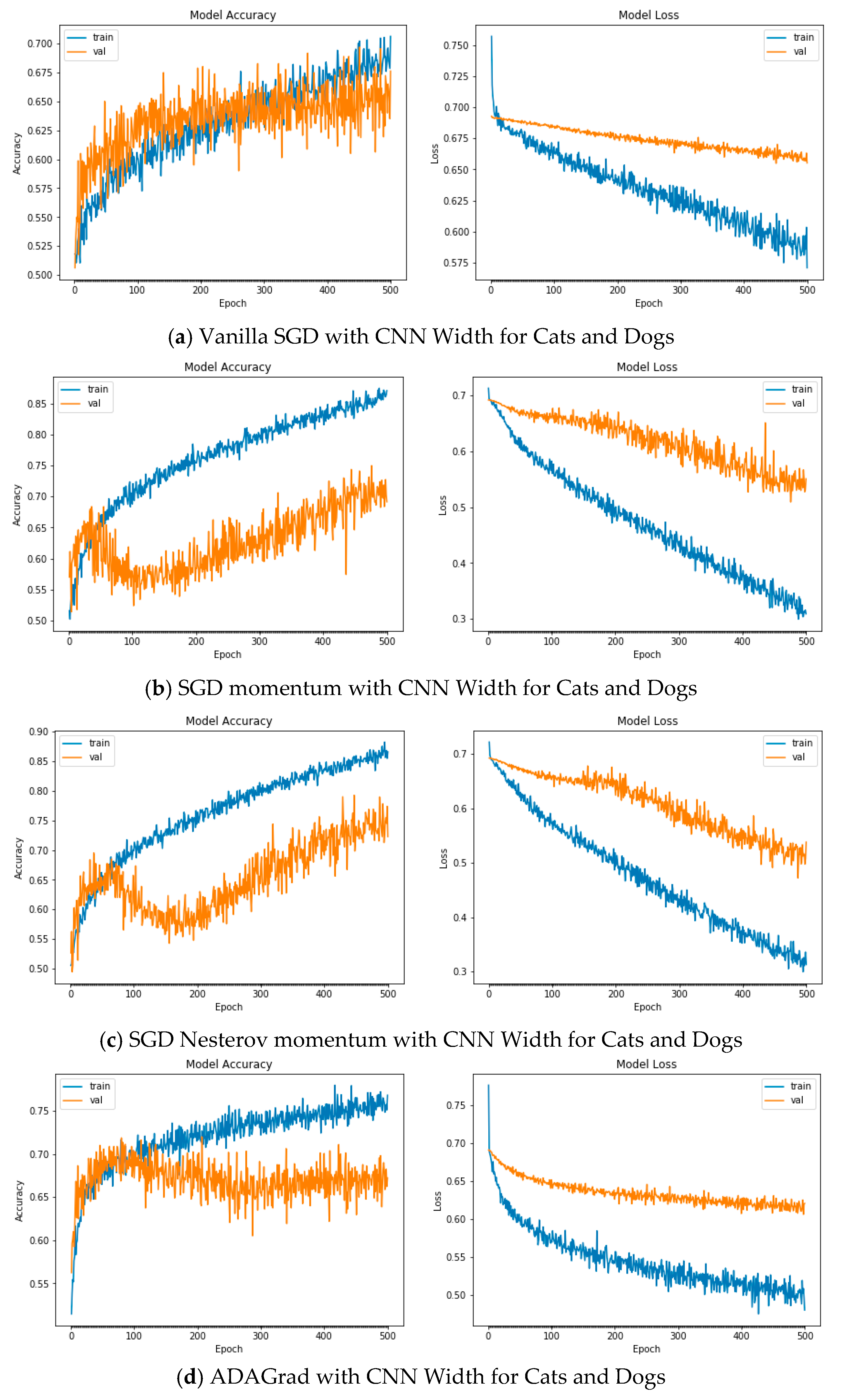
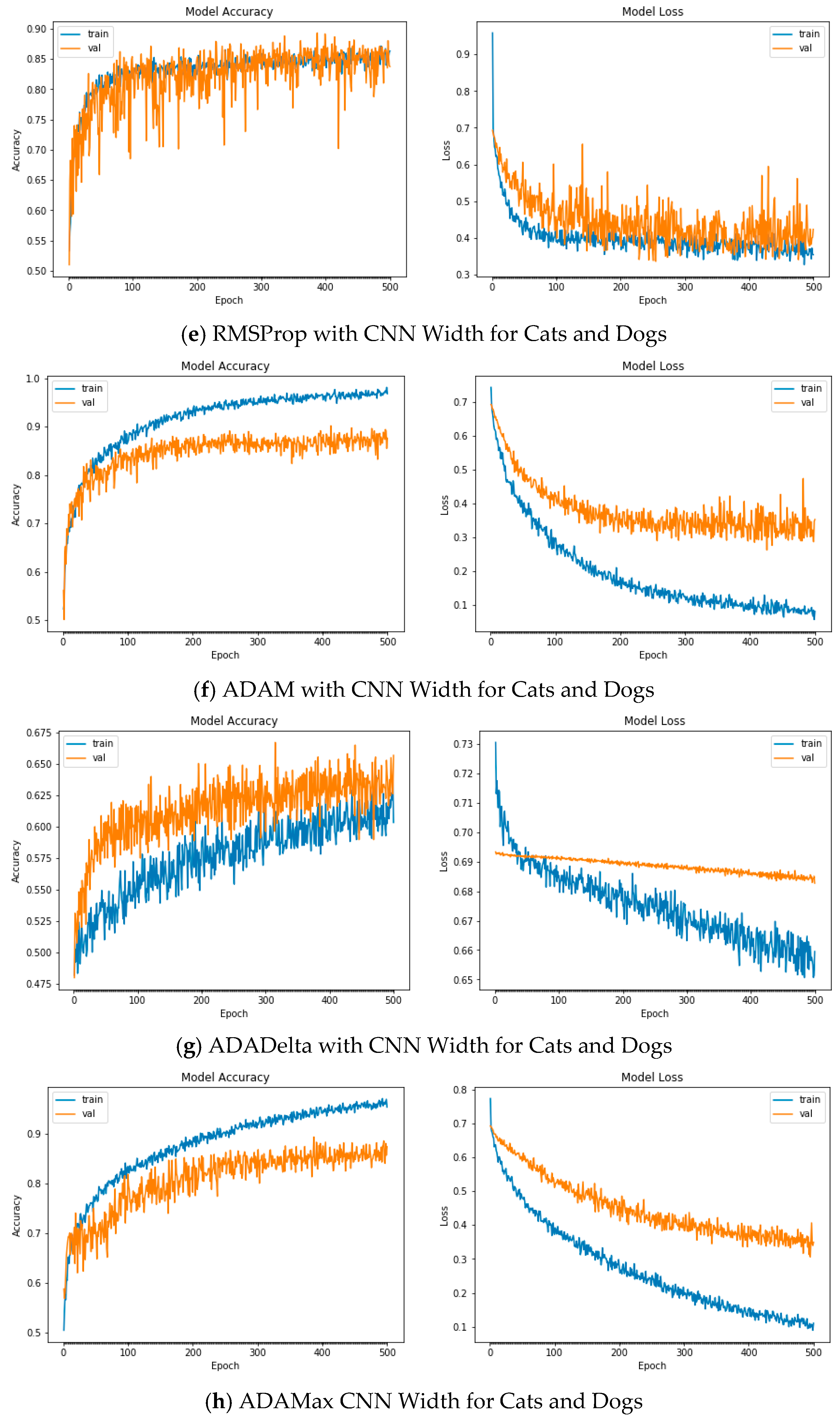
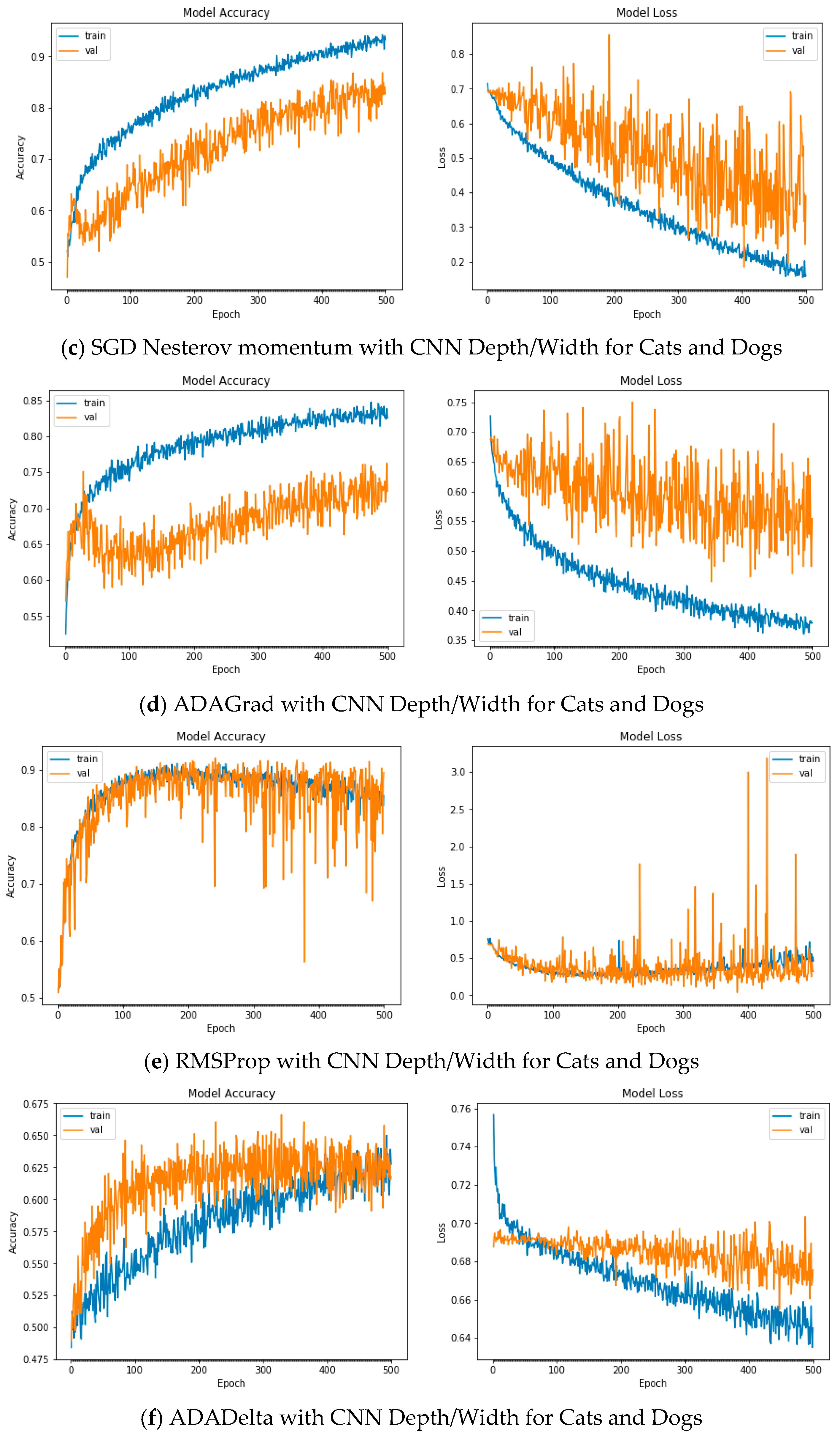
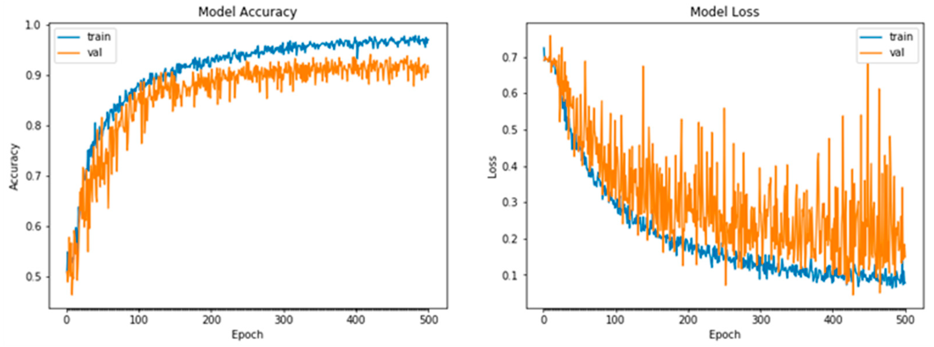
The results obtained for the Cats and Dogs dataset are reported in Table 8. ADAM, in combination with the depth/width CNN model, achieved the best performance in terms of validation accuracy across the three CNN architectures at 91.1%, followed closely by ADAMax (88.9%), RMSProp (87.7%) and NADAM (86.5%), although with variations for convergence time and loss. The other remaining optimizers did not have any significant performance improvements when compared to the simple CNN, except marginal improvements with validation convergence time for NADAM on depth CNN model and better validation loss for RSMSProp on depth/with CNN. The overall worst performers were ADADelta and vanilla SGD. Figure 1 shows plots of train and validation test accuracy and loss against epoch on the best-performing configuration with ADAM and increasing CNN depth/width. More details of all the experimental plots for CNN with varying network sizes for Cats and Dogs are reported in Figure A1 of Appendix A.1, Figure A5 of Appendix B.1 and Figure A7 of Appendix C.1. We noticed no significant improvement after about 500 epochs.

Figure 1. Plot of best-performing ADAM with increasing CNN depth and width on Cats and Dogs.

5.2. Effect of Optimizers with Varying Network Sizes on Natural Images

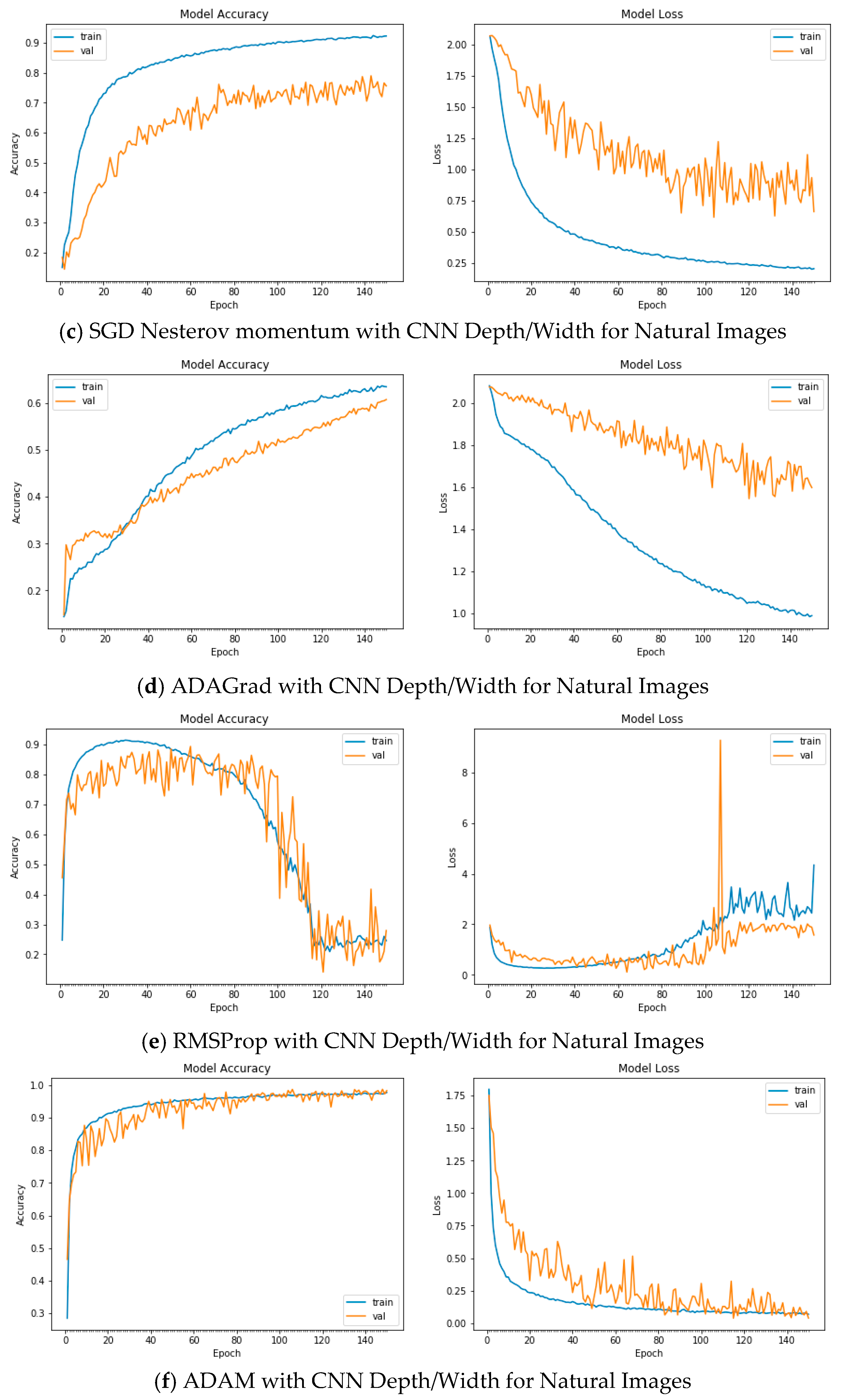
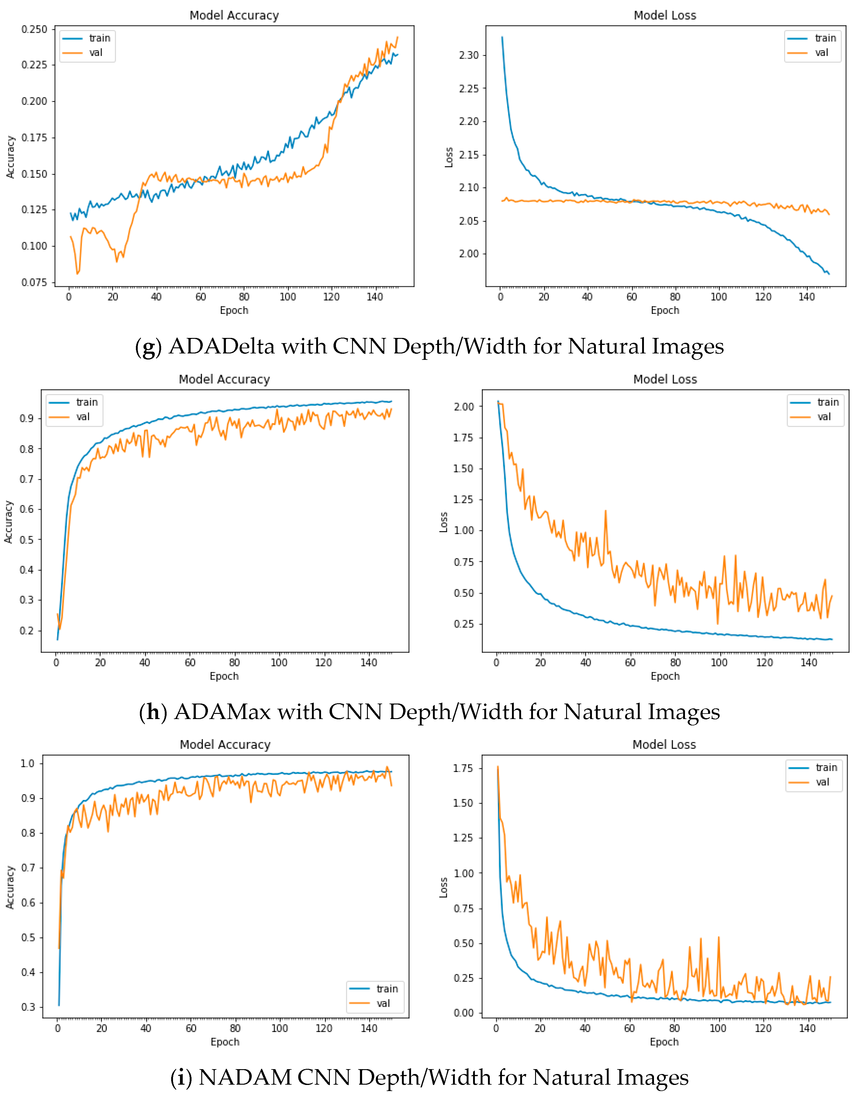
Table 9 reports the results obtained using the Natural Images dataset. ADAM exhibited superior performance with the wider CNN models in terms of validation accuracy at 98.1%, closely followed by NADAM at 97.6%, but at the expense of higher convergence time. ADADelta was still the worst performer in terms of validation accuracy across the CNN models, and in addition, no improvement was noticed compared to the results that were obtained on the simple CNN model. We noticed improved validation accuracy across all the optimizers on the wider CNN model, notably with ADAMax, SGD momentum and SGD Nesterov momentum. Figure 2 shows plots of accuracy and loss against epoch for the best-performing configuration with ADAM and increasing CNN width. In Figure A2 in Appendix A.2, Figure A5 in Appendix B.2, and Figure A8 in Appendix C.2, there are more details of all the experimental plots for CNN with varying network sizes for Natural Images. We noticed no improvement after about 150 epochs.

Figure 2. Plot of best-performing ADAM with increasing CNN width for Natural Images.

5.3. Effect of Optimizers with Varying Network Sizes on Fashion MNIST

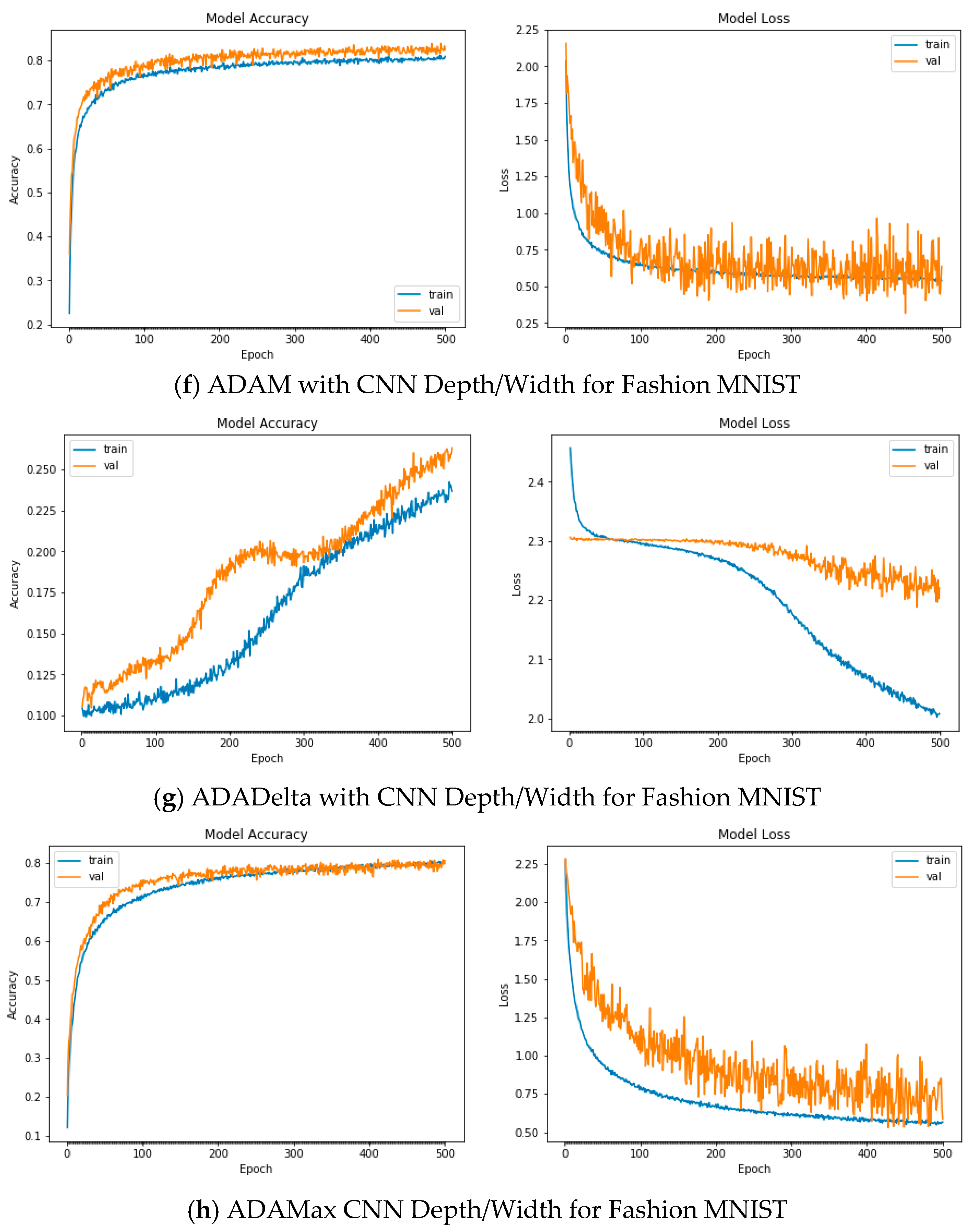
Table 10 reports the results obtained for Fashion MNIST. NADAM was the overall best performer in terms of validation accuracy (83.1%) and loss (0.585) on the depth/width CNN model, followed by ADAM (80.4%) in second position, once again at the expense of higher convergence time. However, ADAM recorded better convergence time when compared to its closest rival, NADAM, on the depth CNN model, with lower accuracy and higher loss. ADADelta was the overall worst performer across all the CNN models for this dataset. Figure 3 shows plots of accuracy and loss against epoch on the best-performing configuration with NADAM and increasing CNN depth/width. In Figure A3 in Appendix A.3, Figure A6 in Appendix B.3, and Figure A9 in Appendix C.3, there are more details of all the experimental plots for CNN with varying network sizes for Fashion MNIST. We noticed no significant improvement after about 500 epochs.

Figure 3. Plot of best-performing NADAM with increasing CNN depth + width on Fashion MNIST.

In this study, the following inferences are drawn based on the results obtained:

• Overall, all the optimizers showed improved performance, particularly ADAM with an accuracy of 91.1% with the deeper/wider CNN architecture for the two-class Cats and Dogs dataset problem. It is, however, worth noting that ADAMax with an accuracy of 88.9% performed marginally better than NADAM with an accuracy of 86.5% with the deeper/wider CNN architecture on Cats and Dogs. This indicates that the incorporated Nesterov momentum in NADAM had little effect on this dataset problem.
• For Natural Images with eight classes, the results show that the wider network architecture generally had better validation accuracy across all the optimizers, especially ADAM with an accuracy of 98.1%, when compared to the simple, deeper, and deeper/wider networks. However, the improved validation accuracy was at the expense of higher convergence time, especially for the adaptive learning rate optimizers. The only exception was ADADelta, which generally performed poorly on this dataset.
• It is worth noting that SGD momentum and SGD Nesterov momentum with the wider CNN architecture performed well on Natural Images with accuracies of 92.9% and 93.7%, respectively. This is consistent with previous studies suggesting that vanilla SGD optimizer can be improved with momentum and Nesterov momentum, and that the improved SGD can be competitive with the adaptive learning rate optimizers for some specific tasks, but with additional time to converge.
• For Fashion MNIST, NADAM was the better performer with an accuracy of 83.1% on depth/width CNN. However, we noted that for the Fashion MNIST there was generally a reduced performance across all the optimizers combined with the CNN architectures. This could be related to the higher number of classes and the simple network design considered in this study.
• The initial results obtained suggest that for the two-class problems, ADAM is a better optimizer to consider with a deeper/wider CNN architecture. For the larger number of classes, ADAM and NADAM with wider networks or deeper/wider network architectures irrespective of dataset size could be considered. However, because of the empirical evidence in the literature that the performance of deeper network tends to worsen after a certain critical point, in addition to increased computational cost due to increased parameterization, a careful balance between depth and width should be applied during the design of deeper/wider CNN architectures. For the majority of tasks, we suggest increasing the width while keeping the depth constant, especially when depth has reached a critical performance point.
• The study demonstrated empirically that significant differences do exist in the performance outputs of different optimizers on varying depth, width and depth/width CNN models, depending on the dataset problem. This is most likely because of their distinctive characteristics and influence on the ability of the CNN models in learning internal representations.
• Finally, from the results obtained, we observed that the optimizers exhibited significant differences in the performance outputs with the wide, deep and deep/wide models. However, the deeper architecture showed an increased risk of poor performance compared to wider and deeper/wider architecture during validation testing. This finding is consistent with previous studies.

6. Conclusions

The objective of the paper was to assess the effects of different optimizers on varying depth and width of CNN architectures. To this end, we conducted an empirical comparison of nine stochastic gradient-based optimization algorithms against three simple CNN architectures of varying depth, width and depth/width, using three image classification dataset problems. Our study reveals that for the Cats and Dogs data problems, ADAM performed remarkably well, much better than its closest rival, NADAM, even though ADAM had a slightly higher convergence time. For the Natural Images data problem, NADAM consistently performed better across all the CNN models. Overall, the worst performer by far was ADADelta across all the models and datasets. For the Fashion MNIST data problem, NADAM was the better performer, but once again, with a slightly higher convergence time than its closest rival ADAM. On the whole, considering the three image classification datasets evaluated, ADAM and NADAM with wider or deeper/wider CNN models were the better performers in terms of accuracy, but at the expense of higher convergence time, while the deeper CNN models generally showed increased performance risk. In this paper, we only looked at three datasets, default settings for the optimizers, and simple CNN architectures. An interesting future direction to pursue is to consider several image classification dataset problems in terms of structure, size, and the number of classes, in addition to hyperparameter tuning of the optimizers and modern CNN architectures. It will also be of interest to investigate the effect of noise from the data images on the prediction accuracies of CNN models, and how robust the CNN models are against noise. However, from the initial results and empirical evidence obtained in this study, we suggest a careful balance between increasing depth and width during the design of deeper/wider CNN architectures, and to try ADAM, NADAM, ADAMax, and SGD with Nesterov momentum as a starting point for image classification problems.

Appendix A.1. Cats and Dogs

Figure A1. Plots of Train and Validation Test accuracies and losses of the CNN model with varying depth for Cats and Dogs: (a) Vanilla SGD; (b) SGD momentum; (c) SGD Nesterov momentum; (d) ADAGrad; (e) RSMProp; (f) ADAM; (g) ADADelta; (h) ADAMax; (i) NADAM.

Appendix A.2. Natural Images

Figure A2. Plots of Train and Validation Test accuracies and losses of the CNN model with varying depth for Natural Images: (a) Vanilla SGD; (b) SGD momentum; (c) SGD Nesterov momentum; (d) ADAGrad; (e) RSMProp; (f) ADAM; (g) ADADelta; (h) ADAMax; (i) NADAM.

Appendix A.3. Fashion MNIST

Figure A3. Plots of Train and Validation Test accuracies and losses of the CNN model with varying depth for Fashion MNIST: (a) Vanilla SGD; (b) SGD momentum; (c) SGD Nesterov momentum; (d) ADAGrad; (e) RSMProp; (f) ADAM; (g) ADADelta; (h) ADAMax; (i) NADAM.

Appendix B.1. Cats and Dogs

Figure A4. Plots of Train and Validation Test accuracies and losses of the CNN model with varying width for Cats and Dogs: (a) Vanilla SGD; (b) SGD momentum; (c) SGD Nesterov momentum; (d) ADAGrad; (e) RSMProp; (f) ADAM; (g) ADADelta; (h) ADAMax; (i) NADAM.

Appendix B.2. Natural Images

Figure A5. Plots of Train and Validation Test accuracies and losses of the CNN model with varying width for Natural Images: (a) Vanilla SGD; (b) SGD momentum; (c) SGD Nesterov momentum; (d) ADAGrad; (e) RSMProp; (f) ADADelta; (g) ADAMax; (h) NADAM.

Appendix B.3. Fashion MNIST

Figure A6. Plots of Train and Validation Test accuracies and losses of the CNN model with varying width for Fashion MNIST: (a) Vanilla SGD; (b) SGD momentum; (c) SGD Nesterov momentum; (d) ADAGrad; (e) RSMProp; (f) ADAM; (g) ADADelta; (h) ADAMax; (i) NADAM.

Appendix C.1. Cats and Dogs

Figure A7. Plots of Train and Validation Test accuracies and losses of the CNN model with varying depth/width for Cats and Dogs: (a) Vanilla SGD; (b) SGD momentum; (c) SGD Nesterov momentum; (d) ADAGrad; (e) RSMProp; (f) ADADelta; (g) ADAMax; (h) NADAM.

Appendix C.2. Natural Images

Figure A8. Plots of Train and Validation Test accuracies and losses of the CNN model with varying depth/width for Natural Images: (a) Vanilla SGD; (b) SGD momentum; (c) SGD Nesterov momentum; (d) ADAGrad; (e) RSMProp; (f) ADAM; (g) ADADelta; (h) ADAMax; (i) NADAM.

Appendix C.3. Fashion MNIST

Figure A9. Plots of Train and Validation Test accuracies and losses of the CNN model with varying depth/width for Fashion MNIST: (a) Vanilla SGD; (b) SGD momentum; (c) SGD Nesterov momentum; (d) ADAGrad; (e) RSMProp; (f) ADAM; (g) ADADelta; (h) ADAMax.

References

1. Papamakarios, G. Comparison of Stochastic Optimization Algorithms. University of Edinburgh: Edinburgh, Scotland, 2014. [Google Scholar]
2. Hallen, R. A Study of Gradient-Based Algorithms. 2017. Available online: http://lup.lub.lu.se/student-papers/record/8904399 (accessed on 20 September 2022).
3. Ruder, S. An overview of gradient descent optimization algorithms. arXiv 2016, arXiv:1609.04747. [Google Scholar]
4. Shalev-Shwartz, S.; Shamir, O.; Shammah, S. Failures of gradient-based deep learning. In Proceedings of the 34th International Conference on Machine Learning, Sydney, Australia, 6–11 August 2017; pp. 3067–3075. [Google Scholar]
5. Tschoepe, M. Beyond SGD: Recent Improvements of Gradient Descent Methods. Master’s Thesis, Technische Universität Kaiserslautern, Kaiserslautern, Germany, 2019. [Google Scholar] [CrossRef]
6. Zhang, M.; Lucas, J.; Ba, J.; Hinton, G.E. Lookahead optimizer: K steps forward, 1 step back. In Advances in Neural Information Processing Systems; MIT: Cambridge, MA, USA, 2019; Volume 32. [Google Scholar]
7. Zhu, A.; Meng, Y.; Zhang, C. An improved Adam Algorithm using look-ahead. In Proceedings of the 2017 International Conference on Deep Learning Technologies, Chengdu, China, 2–4 June 2017; Association for Computing Machinery: New York, NY, USA, 2017; pp. 19–22. [Google Scholar]
8. Reddi, S.J.; Kale, S.; Kumar, S. On the convergence of adam and beyond. arXiv 2019, arXiv:1904.09237. [Google Scholar]
9. Sutskever, I.; Martens, J.; Dahl, G.; Hinton, G. On the importance of initialization and momentum in deep learning. In Proceedings of the 30th International Conference on Machine Learning, Atlanta, GA, USA, 16–21 June 2013; pp. 1139–1147. [Google Scholar]
10. Schaul, T.; Antonoglou, I.; Silver, D. Unit tests for stochastic optimization. arXiv 2013, arXiv:1312.6055. [Google Scholar]
11. Liu, L.; Jiang, H.; He, P.; Chen, W.; Liu, X.; Gao, J.; Han, J. On the variance of the adaptive learning rate and beyond. arXiv 2019, arXiv:1908.03265. [Google Scholar]
12. Rumelhart, D.E.; Hinton, G.E.; Williams, R.J. Learning Internal Representations by Error Propagation. In Parallel Distributed Processing: Explorations in the Microstructure of Cognition: Foundations; MITP: Mainz, Germany, 1987; pp. 318–362. [Google Scholar]
13. Nielsen, M.A. Neural Networks and Deep Learning; Determination Press: San Francisco, CA, USA, 2015; Volume 25. [Google Scholar]
14. Dogo, E.M.; Afolabi, O.J.; Nwulu, N.I.; Twala, B.; Aigbavboa, C.O. A comparative analysis of gradient descent-based optimization algorithms on convolutional neural networks. In Proceedings of the 2018 International Conference on Computational Techniques, Electronics and Mechanical Systems (CTEMS), Belgaum, India, 21–22 December 2018; IEEE: Piscataway, NJ, USA, 2018; pp. 92–99. [Google Scholar]
15. Joshua, A.O.; Nelwamondo, F.V.; Mabuza-Hocquet, G. Segmentation of optic cup and disc for diagnosis of glaucoma on retinal fundus images. In Proceedings of the 2019 Southern African Universities Power Engineering Conference/Robotics and Mechatronics/Pattern Recognition Association of South Africa (SAUPEC/RobMech/PRASA), Bloemfontein, South Africa, 28–30 January 2019; IEEE: Piscataway, NJ, USA, 2019; pp. 183–187. [Google Scholar]
16. Afolabi, O.J.; Mabuza-Hocquet, G.P.; Nelwamondo, F.V.; Paul, B.S. The use of U-Net lite and Extreme Gradient Boost (XGB) for glaucoma detection. IEEE Access 2021, 9, 47411–47424. [Google Scholar] [CrossRef]
17. Yu, Y.; Liang, S.; Samali, B.; Nguyen, T.N.; Zhai, C.; Li, J.; Xie, X. Torsional capacity evaluation of RC beams using an improved bird swarm algorithm optimised 2D convolutional neural network. Eng. Struct. 2022, 273, 115066. [Google Scholar] [CrossRef]
18. Yu, Y.; Samali, B.; Rashidi, M.; Mohammadi, M.; Nguyen, T.N.; Zhang, G. Vision-based concrete crack detection using a hybrid framework considering noise effect. J. Build. Eng. 2022, 61, 105246. [Google Scholar] [CrossRef]
19. Wilson, A.C.; Roelofs, R.; Stern, M.; Srebro, N.; Recht, B. The marginal value of adaptive gradient methods in machine learning. In Advances in Neural Information Processing Systems; MIT: Cambridge, MA, USA, 2017; Volume 30. [Google Scholar]
20. Belkin, M.; Hsu, D.; Ma, S.; Mandal, S. Reconciling modern machine-learning practice and the classical bias–variance trade-off. Proc. Natl. Acad. Sci. USA 2019, 116, 15849–15854. [Google Scholar] [CrossRef]
21. Nichani, E.; Radhakrishnan, A.; Uhler, C. Do deeper convolutional networks perform better? In Proceedings of the International Conference on Machine Learning, Online, 18–24 July 2021. [Google Scholar]
22. Nguyen, T.; Raghu, M.; Kornblith, S. Do wide and deep networks learn the same things? Uncovering how neural network representations vary with width and depth. arXiv 2020, arXiv:2010.15327. [Google Scholar]
23. Tan, M.; Le, Q. Efficientnet: Rethinking model scaling for convolutional neural networks. In Proceedings of the International Conference on Machine Learning, Long Beach, CA, USA, 9–15 June 2019; pp. 6105–6114. [Google Scholar]
24. Hastie, T.; Tibshirani, R.; Friedman, J.H.; Friedman, J.H. The Elements of Statistical Learning: Data Mining, Inference, and Prediction; Springer: New York, NY, USA, 2009; Volume 2, pp. 1–758. [Google Scholar]
25. Yang, Z.; Yu, Y.; You, C.; Steinhardt, J.; Ma, Y. Rethinking bias-variance trade-off for generalization of neural networks. In Proceedings of the International Conference on Machine Learning, Online, 13–18 July 2020; pp. 10767–10777. [Google Scholar]
26. Neyshabur, B. Towards learning convolutions from scratch. In Advances in Neural Information Processing Systems; MIT: Cambridge, MA, USA, 2020; Volume 33, pp. 8078–8088. [Google Scholar]
27. Urban, G.; Geras, K.J.; Kahou, S.E.; Aslan, O.; Wang, S.; Caruana, R.; Richardson, M. Do deep convolutional nets really need to be deep and convolutional? arXiv 2016, arXiv:1603.05691. [Google Scholar]
28. Nguyen, Q.; Hein, M. Optimization landscape and expressivity of deep CNNs. In Proceedings of the International Conference on Machine Learning, Stockholm, Sweden, 10–15 July 2018; pp. 3730–3739. [Google Scholar]
29. Keskar, N.S.; Socher, R. Improving generalization performance by switching from adam to sgd. arXiv 2017, arXiv:1712.07628. [Google Scholar]
30. Choi, D.; Shallue, C.J.; Nado, Z.; Lee, J.; Maddison, C.J.; Dahl, G.E. On empirical comparisons of optimizers for deep learning. arXiv 2019, arXiv:1910.05446. [Google Scholar]
31. Nado, Z.; Gilmer, J.M.; Shallue, C.J.; Anil, R.; Dahl, G.E. A large batch optimizer reality check: Traditional, generic optimizers suffice across batch sizes. arXiv 2021, arXiv:2102.06356. [Google Scholar]
32. Goodfellow, I.; Bengio, Y.; Courville, A. Deep Learning; MIT: Cambridge, MA, USA, 2016. [Google Scholar]
33. Li, H.; Xu, Z.; Taylor, G.; Studer, C.; Goldstein, T. Visualizing the loss landscape of neural nets. arXiv 2017, arXiv:1712.09913. [Google Scholar]
34. Bottou, L. Large-scale machine learning with stochastic gradient descent. In Proceedings of the COMPSTAT’2010: 19th International Conference on Computational Statistics, Paris, France, 22–27 August 2010; Physica-Verlag HD.: Heidelberg, Germany, 2010; pp. 177–186. [Google Scholar]
35. Duchi, J.; Hazan, E.; Singer, Y. Adaptive subgradient methods for online learning and stochastic optimization. J. Mach. Learn. Res. 2011, 12, 2121–2159. [Google Scholar]
36. Tieleman, T.; Hinton, G. Lecture 6.5-rmsprop: Divide the gradient by a running average of its recent magnitude. In Neural Networks for Machine Learning; COURSERA: Mountain View, CA, USA, 2012; Volume 4, pp. 26–31. [Google Scholar]
37. Kingma, D.P.; Ba, J. Adam: A method for stochastic optimization. arXiv 2014, arXiv:1412.6980. [Google Scholar]
38. Zeiler, M.D. Adadelta: An adaptive learning rate method. arXiv 2012, arXiv:1212.5701. [Google Scholar]
39. Dozat, T. Incorporating Nesterov momentum into Adam. ICLR Workshop 2016, 1, 2013–2016. [Google Scholar]
40. Elson, J.; Douceur, J.R.; Howell, J.; Saul, J. Asirra: A CAPTCHA that exploits interest-aligned manual image categorization. In Proceedings of the 14th ACM Conference on Computer and Communications Security (CCS), CATS/DOGS, Alexandria, VA, USA, 31 October–2 November 2007; Association for Computing Machinery, Inc.: New York, NY, USA, 2007; Volume 7, pp. 366–374. [Google Scholar]
41. Roy, P.; Ghosh, S.; Bhattacharya, S.; Pal, U. Effects of degradations on deep neural network architectures. arXiv 2018, arXiv:1807.10108. [Google Scholar]
42. Xiao, H.; Rasul, K.; Vollgraf, R. Fashion-mnist: A novel image dataset for benchmarking machine learning algorithms. arXiv 2017, arXiv:1708.07747. [Google Scholar]
43. Khan, A.; Sohail, A.; Zahoora, U.; Qureshi, A.S. A survey of the recent architectures of deep convolutional neural networks. Artif. Intell. Rev. 2020, 53, 5455–5516. [Google Scholar] [CrossRef]
44. Shrestha, A.; Mahmood, A. Review of deep learning algorithms and architectures. IEEE Access 2019, 7, 53040–53065. [Google Scholar] [CrossRef]
45. Alzubaidi, L.; Zhang, J.; Humaidi, A.J.; Al-Dujaili, A.; Duan, Y.; Al-Shamma, O.; Farhan, L. Review of deep learning: Concepts, CNN architectures, challenges, applications, future directions. J. Big Data 2021, 8, 1–74. [Google Scholar] [CrossRef] [PubMed]
Publisher’s Note: MDPI stays neutral with regard to jurisdictional claims in published maps and institutional affiliations.
Article Metrics
Citations
Article Access Statistics
Multiple requests from the same IP address are counted as one view.