Abstract
Bearings are key components in modern power machines. Effective diagnosis of bearing faults is crucial for normal operation. Recently, the deep convolutional neural network (DCNN) with 2D visualization technology has shown great potential in bearing fault diagnosis. Traditional DCNN-based fault diagnosis mostly adopts a single learner with one input and is time-consuming in sample and network construction to obtain a satisfied performance. In this paper, a scheme combining diverse DCNN learners and an AdaBoost tree-based ensemble classifier is proposed to improve the diagnosis performance and reduce the requirement of sample and network construction simultaneously. In this scheme, multiple types of samples can be constructed independently and employed for diagnosis simultaneously; next, the same number of DCNN learners are built for underlying features extraction and the obtained results are integrated and finally fed into the ensemble classifier for fault diagnosis. An illustration based on the Case Western Reserve University datasets is given, which proves the superiority of the proposed scheme in both accuracy and robustness. Herein, we present a universal scheme to improve the diagnosis performance, and give an example for practical application, where the signal preprocessing and image sample construction methods can also be applied in other vibration-based analysis.
1. Introduction
Bearings are important to any processing or manufacturing plant that uses rotating equipment. Unfortunately, however, many bearings fail prematurely in service because of contamination, poor lubrication, misalignment, temperature extremes, poor fitting/fits, shaft unbalance, and misalignment. All of these factors lead to an increase in bearing vibration and may show typical patterns in spectrum. It is essential to have a spectrum of vibration of bearings to diagnose the source of evolving fault(s) for preventive maintenance, as bearings are the most common elements in rotating machinery and with a large number in any factory. Therefore, their failure often leads to unacceptably long production downtimes [1,2,3], and it is important to monitor any potential source of evolving bearing fault. Due to the reasons above, bearing fault diagnosis is receiving more and more attention.
The vibration of rolling bearings results from external forces of machine system, i.e., an unbalance of forces, or bearings act as the excitation sources producing time varying forces that cause system vibration. As for the latter, the components of rolling bearings, i.e., rolling element, inner raceway, outer raceway, and cage interact to generate complex vibration. The sources of vibration include variable compliance [4] and geometrical imperfections (e.g., surface roughness [5] and waviness [6,7]), and some of these show typical effects in a spectrum [8]. For example, the increased amplitude at ball or roller pass frequency indicates emerging clearances in bearings or loss of loading, and that of ball spin or at cage rotational frequency gives a signature of cage slipping or collisions. Thus, as stated above, it is essential to have a spectrum of vibration of bearings to diagnose the source of evolving fault(s). However, the vibration signals are usually affected by the variable operating conditions and background noise, which lead to the diversity and complexity of the vibration signal characteristics, and it is a challenge to effectively identify the bearing faults from such vibration signals without further fault information. Thus, it is of significance to extract the fault-related features embedded in the raw signals. In the past few decades, many methods have been developed for feature extraction. Generally, features can be extracted from signals in time domain [9,10], frequency domain [11,12], and time-frequency domain [13,14,15]. In the time domain, the dimensional statistical indices (e.g., root mean square value and central moment) and dimensionless statistical indices (e.g., skewness and kurtosis) are commonly used that achieve good results. In the view of frequency and time-frequency domains, the vibration signals of the rolling element bearing usually contain a rich spectrum. Different defect positions, such as outer race, inner race, and the ball, have a corresponding fault characteristic frequency. Based on this, some useful methods including the Fast Fourier Transform (FFT), Envelope Spectrum, Short-time Fourier Transform (STFT), Wavelet Transform (WT) [13], and Empirical Mode Decomposition (EMD) [14] have been developed for feature selection and are proved effective in determining existing faults and classifying failure modes of mechanical systems. Rai et al. [16] carried out bearing fault diagnosis by combining FFT and Hilbert–Huang transform. In this study, the transformation results of HHT were further processed by FFT. It was verified that the proposed method could clearly indicate the effectiveness of fault-related frequencies and improve the robustness of diagnosis. Gao et al. [17] employed STFT and non-negative matrix factorization to extract features for rolling bearing fault recognition. STFT was used to acquire the time-frequency distribution of raw signals. The recognition results yielded a higher accuracy than traditional ANN methods. Ali et al. [18] made an effort to characterize and classify seven different bearing classes, where EMD is applied to perform primarily processing on the non-stationary vibration signals. The energy entropy is then calculated on each of the obtained intrinsic mode functions (IMFs) and used as features for classification. Guo et al. [19] proposed a novel signal compression method for bearing vibration signals where the ensemble empirical mode decomposition method is employed for separating fault-related signal components from irrelevant ones. The results proved that the proposed method provided a higher compression ratio, while retaining the bearing defect characteristics. Vafaei et al. [20] developed a new signal processing method by combining indicated runout with wavelet decomposition, which was employed to effectively window around regions of interest with the indicated runout method. An example in the paper showed that the method could pinpoint with remarkable accuracy the physical cause of the vibration response. Huo et al. [21] used the impulse modeling continuous wavelet transform (IMCWT) model to diagnose bearing faults under multi-speed, where quasi-Newton optimization algorithms were applied to optimize IMCWT model so that fault information from vibration signals could be extracted more effectively. However, on one hand, the above studies need careful engineering and substantial domain expertise in selecting the useful features related to faults, and on the other hand, information of single domain, such as time-frequency domain, is mostly adopted for fault diagnosis and the time domain and frequency domain information are not considered. These have limited the further development of fault diagnosis especially with the growth of complexity of mechanical systems and computation requirements.
In recent years, with the achievement in deep learning and computation ability, the data-driven methods accompanied with the 2D visualization technique [22,23,24] for feature selection are widely developed and show excellent performance in fault diagnosis. Deep Convolutional Neural Network is one of the most used deep learning structures that has been gaining more and more attention, particularly in the field of image processing [25], pattern analysis [26], and fault diagnosis [27,28,29]. For the DCNN-based fault diagnosis, data are primarily processed and transformed into 2D samples as the input of classifier, and the final features for decision-making are obtained by iterations of self-study and not dependent on manual selection. One effective method for primary data processing is to make transformations on the data in time domain, frequency domain, and time-frequency domain to obtain related features which are further used for sample construction. However, as stated above, features of single domain are adopted for fault diagnosis in many earlier studies, which only describe the specific aspect of vibration signals, and with the rich features of the raw signals it is not easy to figure out the domain(s) where features give the most contribution to the fault diagnosis. On this account, some works combine features from more than one domain for a better fault diagnosis performance. For example, Roozbeh et al. [30] carried out diagnosis on gear faults, where features are first extracted from the sensor measurements in frequency domain and time-frequency domain by corresponding tools such as FFT and WPT, and statistics are then calculated on the obtained results, after which all the features are fused in sequence as the input of diagnosis scheme where DCNN is used. Zhao et al. [31] extracted features in the time domain (statistical induces), frequency domain (spectral skewness and kurtosis), and time-frequency domain (wavelet energy) for reducing the dimension of raw signals. The obtained results are then used for machine health monitoring.
For most of studies on DCNN-based fault diagnosis, a single network is used, which means there is only one input. This leads to the problem of features integration across different domains, in other words, a careful construction of sample is needed to contain useful information as much as possible. However, the analysis results of raw signals may have different dimensions in different domains, due to which features in different domains cannot be fused directly. For example, the transformation results of raw signal by FFT and WT are [frequency × amplitude] and [time × frequency × amplitude], corresponding to frequency domain and time-frequency domain, respectively. Beside those mentioned above, in single DCNN-based fault diagnosis, plenty of work must be done with respect to structure designing and parameter tuning to obtain a satisfying performance (e.g., diagnosis accuracy). This is generally done by running multiple trials where each trial is a complete execution of training application with values for the chosen structure and hyperparameters and is time-consuming. There is not a common approach applicable for all cases to provide a theoretical guide on this process, so situations may arise in which the performance of the deep learning network is hard to be improved by personal expertise.
Considering the problems above, we propose a scheme that combines diverse CNN learners and AdaBoost tree-based ensemble classifier. The information of raw signals in the time domain, frequency domain, and time-frequency domain are employed in the form of 2D images for diagnosis. Differently, samples are constructed separately and contribute to fault diagnosis simultaneously, which eliminates the situation that only one domain is focused or an elaborate feature integration across different domains must be determined in traditional vibration-based fault diagnosis, thus providing more freedom for the sample construction where each type of sample can concentrate on one aspect of the signal. To our best knowledge, although there were some studies assembling CNNs and the AdaBoost algorithm-based classifier [32,33,34] for classification, proving its effect in improving classification accuracy, few researches have paid attention to the change of this improvement and the robustness of such an ensemble method. Herein, we present a universal framework to improve the diagnosis performance, and give instruction for the practical application of the framework where the proposed methodologies for 2D sample construction in this paper can also be applied in other vibration-based analysis.
2. Feature Extraction in Multiple Domains
2.1. Feature Extraction in the Time Domain
The statistical methods are widely used to capture key process characteristics that reveal the hidden information of the signal. In traditional ways, the statistics are computed upon the whole sample, losing the time-varied features of non-stationary signals. To overcome this problem, a window-based continuous statistical analysis (CSA) method is proposed to obtain the statistic patterns of a sample in a time scale where the output is time series as shown in Figure 1.
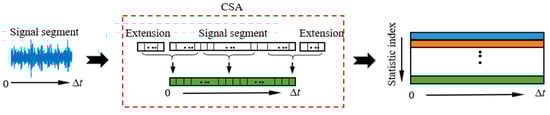
Figure 1.
The process of continuous statistical analysis.
When a signal with a time length of Δt passes through the continuous statistical analysis, it is converted into several time sequences where each sequence corresponds to a statistic index, e.g., skewness. In this process, a point of the output time sequence is obtained by statistics over a certain width of data region with this point as the center. Instead of calculating over the whole sample, the results by this method are time-dependent, given as
where sta(t)i,j donates the time series corresponding to the jth statistic index of the ith sample si, f is the statistic function, t is time, and δt is the region width that keeps constant in the calculation. Symmetric extensions of δt/2 are made on the two ends of the signal, separately, to obtain the results in the borders.
2.2. Feature Extraction in the Frequency Domain
Spectrum analysis is applied to the raw signals for feature extraction in the frequency domain. In this process, the Fast Fourier Transform (FFT) algorithm is used, which breaks the signal down into all its frequencies by computing the Discrete Fourier transform of a sequence. Let X0, X1, …, XN−1 be complex numbers. The Discrete Fourier transform is defined by the formula:
where ei2π/N is a primitive Nth root of 1.
Besides the FFT, Envelope Spectrum Analysis (ESA) is also proved to be effective in extracting periodic impacts from the vibration signal. It can extract impacts with very low energy and even those hidden by other vibration signals, thus it is widely used to detect and diagnose rolling element bearing faults [35], where the vibration becomes amplitude-modulated due to periodic changes in the forces when a fault develops. To obtain the envelope spectrum, the Hilbert Transform (HT) [36], one of the most frequently used methods for envelope analysis, is first performed on the signal. For signal s(t), its Hilbert Transform is defined as
Then, the analytic signal of s(t) can be expressed as
sA(t) is the analytic signal of s(t), which is complex-valued. A(t) is the instantaneous amplitude namely envelope and ψ(t) is the instantaneous phase. Then, FFT is employed on the envelope to obtain the envelope spectrum.
2.3. Feature Extraction in the Time-Frequency Domain
Wavelet analysis is employed to extract features of the raw signals in the time-frequency domain. The continuous wavelet transform (CWT) and discrete wavelet transform (DWT) are two commonly used methods that capture both frequency and location information (location in time) due to its temporal resolution, and have been shown to be effective in faults diagnosis, image processing, and many others. The following gives a brief introduction to the algorithm of CWT and DWT.
The continuous wavelet transform of a vibration signal s(t) at a scale (a > 0) a ϵ R+ and translational value b ϵ R is expressed by the following integral,
where ψa,b(•) is a continuous function in both the time domain and the frequency domain called the mother wavelet and the over line represents the operation of complex conjugate. Then, the wavelet family is generated by dilating and translating a fixed valued wavelet base ψ(b), expressed as
For the discrete wavelet transform (DWT), the Hilbert basis is constructed as the family of functions {ψa,b: a, b∈Z} by means of dyadic translations and dilations of ψ:
Here, a = 2−j is the binary dilation and b = k∙2−j donates the binary position.
The continuous wavelet transform provides an overcomplete representation of a signal by letting the translation and scale parameter of the wavelets vary continuously, whereas in the discrete wavelet transform, the wavelets are discretely sampled. For the nth level of decomposition, the WPT (one of the DWT methods) produces 2n different sets of coefficients, and each set of coefficients can be converted to a time series by signal reconstruction.
3. Proposed Fault Diagnosis Scheme
3.1. Basic Structure of DCNN
Three main types of layers are used to build DCNN architectures, namely, Convolutional Layer (CONV), Pooling Layer, and Fully-Connected Layer (FC), which are stacked to form a full DCNN architecture.
- INPUT holds the raw pixel values of the image with width W and height H in each of the three color channels R, G, and B.
- CONV layer computes the output of neurons that are connected to local regions in the input, each computing a dot product between their weights and a small region they are connected to in the input volume.
- RELU layer applies an element-wise activation function, such as max (0, x), thresholding at zero.
- POOL layer performs a downsampling operation along the spatial dimensions (width, height), which ensures that contribution from the pixels that carry salient information in the feature maps are carried forward and leads to dimensional reduction by making maximum or average operation on the pooling region.
- FC layer computes the class scores, resulting in a volume of size [1×1×m], where each of the m numbers corresponds to a class score. As with ordinary Neural Networks, and as the name implies, each neuron in this layer will be connected to all the numbers in the previous volume.
3.2. Adaptive Boosting Algorithm
AdaBoost (adaptive boosting) is an ensemble learning algorithm that can be used for classification or regression. It is called adaptive because it creates a strong learner (a classifier that is well-correlated to the true classifier) by iteratively adding weak learners (a classifier that is only slightly correlated to the true classifier). Figure 2 illustrates the working principle of AdaBoost classifier.
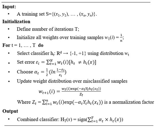
Figure 2.
The working principle of AdaBoost classifier.
AdaBoost.M2 [37] is an extension of AdaBoost. It introduces pseudo-loss, which is a more sophisticated method to estimate error and update the instance weight in each iteration compared with AdaBoost. Given a set of samples S {(x1, y1), …, (xm, ym)} xi ϵ X with labels yi ϵ Y = {1, …, C}, the distribution of samples is initialized as D1(i) = 1/m. The AdaBoost.M2 algorithm proceeds in a series of T rounds. In the tth round, a weak learner Lt is trained using distribution Dt, and the pseudo-loss of weak hypothesis ht: X×Y→[0,1] is computed as
where B = {(i,y): i = 1,…, m, y ≠ yi}. Donate
βt = ɛt/(1 − ɛt),
wt = (1/2) × (1 − ht(xi,yi) + ht(xi,y))
Then, the distribution Dt is updated according to
where Zt is a normalization constant chosen such that Dt+1 is a distribution. After all T rounds are finished, the final hypothesis is given as
The AdaBoost.M2 is used to construct the multiclass classifier for bearing fault diagnosis. The weak learners can be chosen diversely such as Support Vector Machine (SVM) [38], neural networks [39], and decision tree [40]. Among these learners, the decision tree is generally faster to train and does not need parameter tuning, except for specifying the number of trees. Moreover, it avoids the problem of overfitting that has to be considered for neural networks. Therefore, the decision tree is finally chosen as the weak classifier based on which the AdaBoost tree-based ensemble classifier is constructed.
3.3. Hybrid Deep Recognition Scheme
The proposed hybrid deep recognition scheme based on DCNN and AdaBoost tree-based ensemble classifier (called hybrid Ada-DCNN) is presented as Figure 3.
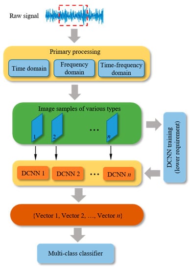
Figure 3.
The proposed hybrid deep recognition scheme (hybrid Ada-DCNN).
In the diagnosis process, the raw signal is divided into segments for processing. Each segment is primarily processed in the time domain, frequency domain time-frequency domain using corresponding tools introduced previously. Based on the obtained results, various types of 2D samples are generated by image processing. Note that the sizes of different types of sample are independent and determined by the dimension of corresponding features. The rest of the proposed scheme is divided into two steps, namely, (1) underlying feature extraction and (2) multiclass classification.
3.3.1. Underlying Feature Extraction
The architecture of DCNN provides a technique for the reduction of input dimension, retaining important features to be learned easily. In this part, a set of DCNNs are built where each DCNN corresponds to one type of sample. The DCNNs are pre-trained until they meet the expected accuracy, which is regarded as an indicator for the feature extraction performance. Differently, achieving the same diagnosis performance, the requirement of accuracy of DCNNs in the proposed scheme is lower than that in traditional single DCNN-based diagnosis as the final performance of diagnosis depends on the assemble effect of DCNNs, which will be demonstrated by following works. In other words, the proposed diagnosis scheme can reduce the work of DCNN construction.
After the training of DCNNs, they perform as extractors over corresponding examples. The activations of the last FC layer are picked up and fused to produce the integrated feature space as below,
where Fea (i) is the integrated feature space corresponding to the ith signal segment, and Sp,q donates the qth element of features obtained from the FC layer of the pth DCNN.
3.3.2. Multiclass Classification
After step (1), the integrated features related to all the samples are produced. Then, the Adaboost tree-based ensemble classifier is constructed for multiclass classification using the obtained enhanced features. The number of trees is determined by iteration. After the classification, a confusion matrix is obtained which presents the classification details in terms of each fault condition. As mentioned above, the AdaBoost tree-based ensemble classifier avoids the problem of overfitting. Furthermore, after integration the feature vector gives consideration of all three domains of the raw signal. For the above reasons, an improved performance can be obtained over traditional single DCNN-based method.
4. Sample Preparation
4.1. Experiment Test
Coupled with the increasing attention on vibration-based diagnosis and prognostics of rolling bearing, providing an open access databases is of more importance than ever before. There are so far several available datasets such as the Case Western Reserve University datasets (CWRU) [41] and University of Cincinnati datasets [42] that can be used to validate or improve the condition assessment and diagnostic techniques. In this paper, the vibration datasets from the CWRU data center are adopted. Vibration data was collected using accelerometers, which were attached to the housing with magnetic bases. Accelerometers were placed at the 12 o’clock position at both the drive end and fan end of the motor housing. Vibration signals were collected using a 16-channel DAT recorder. Speed and horsepower data were collected using the torque transducer/encoder and were recorded by hand.
Figure 4a shows the test stand used for the CWRU datasets.
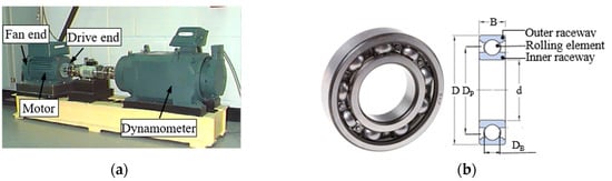
Figure 4.
The test stand and structure of tested rolling element bearing of the Case Western Reserve University (CWRU) datasets: (a) The test stand of CWRU datasets; (b) Structure of the tested bearing in drive end.
The motor bearings are seeded with faults of 0.1778 mm, 0.3556 mm, 0.5334 mm, and 0.7112 mm in diameter introduced at the inner ring (IR), rolling element (RE), and outer ring (OR), separately. The data used in this paper are acceleration signals in the vertical directions on the bearing housing of drive end (DE) recorded by 12,000 samples per second at four rotation speeds: 1797, 1772, 1750, and 1730 RPM. Figure 4b illustrates the structure of the bearing in drive end with parameters in Table 1, where d, D, DB, B, and DP denote inside diameter, outside diameter, ball diameter, thickness, and pitch diameter, respectively.

Table 1.
Bearing size at the drive end (unit: mm) [43].
Based on kinematic relationships assuming no slip, the bearing fault frequencies of IR, OR, and RE are as follows [6,41],
where fr is the shaft speed, n is the number of rolling elements, and is the angle of the load from the radial plane. Table 2 lists the bearing details and fault frequencies at the drive end as the multiple of shaft speed. Taking the raw signals collected at 1797rpm as an example, we give the envelope signals and corresponding envelope spectrum with respect to IR fault, OR fault, and RE fault as Figure 5. The results show the fault frequencies as well as harmonics are in accord with theoretical analysis.
Table 2.
Bearing details and fault frequencies.
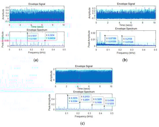
Figure 5.
Envelope signal and corresponding envelope spectrum of raw signals at 1797rpm with respect to (a) IR fault, (b) OR fault, and (c) RE fault.
4.2. Data Processing
According to Table 2, the fault with the highest frequency occurs at the inner raceway with a rotation speed of 1797 RPM (~162.19 Hz), which is far below the sampling frequency of 12,000 Hz. In view of frequency analysis, the fault information usually presents a larger response in the first several orders of fault frequency. Frequency components out of this region help less for the fault diagnosis; on the other hand, a high sampling frequency will lead to a sample of big volume that increases the burden of deep learning. In this paper, the first 4 orders of the highest fault frequency (162.19 × 4 = 648.76 Hz) is considered, accordingly the raw signal is downsampled from 12,000 Hz to 1500 Hz based on the Nyquist Sampling theorem, where the sampling frequency should be two times the highest observation frequency at least (1500/648.76 ≈ 2.3).
The downsampling operation above is based on the resample function embedded in Matlab. It applies an antialiasing FIR low-pass filter to the objective sequence, and compensates for the delay introduced by the filter. Figure 6 shows the comparison of signals as well as corresponding frequencies before and after downsampling. It can be seen that after downsampling, only the components below the highest observation frequency (25.04 as multiple of f0) are reserved. The results are in accord with previous analyses. Besides, an obvious reduction of energy can be found from the raw signals after downsampling according to the change of amplitude. This reduction occurs because that the high-frequency components (above the highest observation frequency) are eliminated from the raw signals.
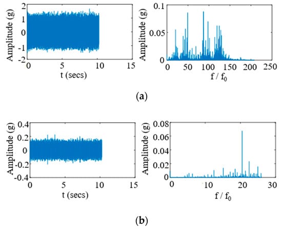
Figure 6.
Comparison of signals as well as the frequency results before and after downsampling: (a) Original signal and frequency results of FFT; (b) Downsampled signal and frequency results of FFT.
4.3. Sample Construction
As presented above, the number and size of samples are not constrained. In this study, for an illustration of the proposed diagnosis scheme, we construct three types of samples based on the primary processed results of raw signal where two focus on single domain (frequency and time-frequency, respectively) and the rest one focuses on three domains simultaneously (time, frequency, and time-frequency), and accordingly three DCNNs are built. Considering the binary decomposition of DWT as well as the limitation of sample volume, the time length of a signal segment is chosen by multiple trials to be about 0.17 s with 256 (28 = 256) points included (256/1500 ≈ 0.17s). Then, the three types of samples are introduced in detail as below.
4.3.1. Sample Construction in the Frequency Domain
A 4-layer Wavelet Packet Transform (WPT) based on the Daubechies wavelet is first performed on the raw signals. As a result, 2i subsequences are generated for the ith layer (I = 1, 2, 3, 4) and each subsequence has a frequency width of (fs/2)/2i, where fs is the sampling frequency. Therefore, there are a total of 31 (1 + 21 + 22 + 23 + 24 = 31) sequences with the raw signal included. Features for sample construction come from two parts: (1) results of FFT on the 31 sequences and (2) results of ESA on the 31 sequences. The output of a sequence in each part is a 128 × 1 vector where the length is half of the sequence. Combining the two parts, a matrix of size 128 × 62 is obtained with respect to a signal segment and the matrix is independent with time. Finally, the obtained matrix is converted into an image by gray processing.
4.3.2. Sample Construction in the Time-Frequency Domain
The CWT is employed on the raw signal to obtain the results in the time-frequency domain, where the Morlet wavelet is chosen as the mother wavelet. In the frequency dimension, we set the scale to be 256, which represents the frequency domain is divided into 256 sub-bands; in time dimension the size matches the length of the input signal. By performing CWT on the raw signal, the wavelet coefficients in the form of 256 × 256 matrix are obtained. Each row of the matrix contains the coefficients for one scale. Finally, the coefficients are converted into an image by gray processing likewise.
4.3.3. Sample Construction in Three-Domains
In this part, we give an integrated sample that contains features in three domains. The 31 subsequences obtained in (1) form the first part of the sample. Then, the 31 subsequences are processed using HT for Envelope Analysis. The time-varied results of HT are directly used as the second part of the sample, which do not pass the FFT analysis so that they can be fused with the first part of the sample, as they have the same size in the time dimension. After that, there are 31 sequences obtained in the Envelope Analysis accordingly. The third part of the sample is generated using the continuous statistical analysis method based on the 31 subsequences in the first part. Eight dimensionless statistic indices, including six general ones listed in Table 3, which are formed by combining the dimensional indices in Table 4, and two energy-related indices (energy ratio and entropy) as in Equations (14) and (15). The six general indices are applied to all 31 subsequences, by which 186 (31 × 6 = 186) sequences are obtained; the energy-related indices are performed on the 16 subsequences of the 4th layer in WPT, and 17 sequences (16 for energy ratio, 1 for entropy) are obtained accordingly. Combining the three parts of the sample, a matrix of size 256 × 265 is acquired and converted into an image by gray processing.
Table 3.
The general dimensionless statistics used for sample construction.
Table 4.
The basic dimensional statistics.
Based on the analysis above, the three types of samples for the bearing faults diagnosis are produced using the datasets. For each type, there are totally 2832 images generated with details listed in Table 5.
Table 5.
Sample numbers of faulty and normal conditions.
Figure 7 presents the example of the three types of samples.
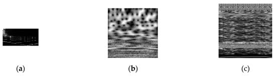
Figure 7.
Three types of image samples corresponding to: (a) Frequency domain, size 128 × 62 (FD); (b) time-frequency domain (TFD), size 256 × 256; and (c) three-domains (ThD), size 256 × 265.
5. Implementation and Results
The bearing fault diagnosis is performed on three fault types (IR, RE, and OR) and the normal condition (NC). In this process, the ratio of the validation dataset is set to be 0.2. The Deep Network Designer embedded in Matlab is employed for the construction, training, and validation of DCNN using a single CUDA-enabled NVIDIA Quadro P4000 GPU.
5.1. Comparison between DCNN and Ada-DCNN
First, the DCNNs corresponding to the three types of samples in Figure 7 are built and denoted as FD-Net, TFD-Net, and ThD-Net, respectively. As an example, the final structure and parameters of the FD-Net is illustrated in Figure 8. Each network is iteratively tuned to specify the structure and hyperparameters such as layer and channel numbers, kernel sizes, and so on. Once the training of DCNNs is completed, the activations of the last FC layer are extracted for the training of the AdaBoost tree-based ensemble classifier. The accuracy of DCNNs is used as an indicator of the feature extraction performance. To compare the diagnosis performance of a DCNN and corresponding Ada-DCNN, four accuracy levels (S1–S4) are achieved for each DCNNs in the validation process.
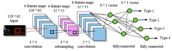
Figure 8.
The final structure and related parameters of FD-Net.
The fault diagnosis performance of a DCNN and corresponding Ada-DCNN are compared under four accuracy levels as in Table 6, and the accuracy of DCNNs, as well as the improvements by Ada-DCNNs in four levels, are shown in Figure 9a.
Table 6.
Comparison between the performance of DCNNs and corresponding Ada-DCNNs under four accuracy levels.
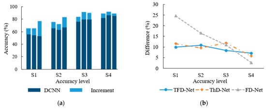
Figure 9.
Comparison between DCNNs and Ada-DCNNs in 4 accuracy levels: (a) Accuracy of DCNNs as well as the increment by Ada-DCNN in 4 accuracy levels; (b) Difference of accuracy between DCNNs and related Ada-DCNNs in 4 accuracy levels.
The results indicate that the diagnosis accuracy of Ada-DCNN is obviously higher than the related DCNN in all accuracy levels. Figure 9b shows the difference of accuracy between the DCNNs and related Ada-DCNNs. It can be seen that the improvement declines with the growing of DCNN accuracy from S1 to S4 for the three networks, which is not difficult to understand as the accuracy increases more slowly when it approaches the ceiling (100%). A further calculation shows that the average accuracy of DCNNs from S1 to S4 is improved by an absolute value of 15.37%, 12.29%, 10.40%, and 5.14%, respectively.
The training details of the DCNNs and classification results of the Ada-DCNNs are not provided due to the limitation of space. As an example, we only give the training and validation processes of FD-Net and the fusion matrix of the corresponding Ada-DCNN in the accuracy level S1 as in Figure 10.
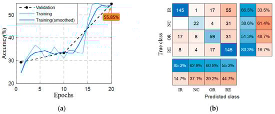
Figure 10.
The detail results of FD-Net in the accuracy level S1: (a) The training and validation process of DCNN (55.85%); (b) The fusion matrix of the related Ada-DCNN (65.78%).
5.2. Comparison between the Ada-DCNN and Hybrid Ada-DCNN
The diagnosis performance of Ada-DCNN is superior to the DCNN in Section 5.1. In this part, we investigate the performance of the hybrid Ada-DCNN and compare it with the DCNN and Ada-DCNN in all the 4 accuracy levels (S1–S4). Under each level, the features are extracted by the DCNNs and integrated as the final feature vector for classification.
We donate [Si, Sj, Sk] as the integration of TFD-Net, ThD-Net, and FD-Net under the ith, jth, and kth accuracy levels, respectively. The accuracy of hybrid Ada-DCNN and the average values of related Ada-DCNNs and DCNNs for each integration are listed in Table 7.
Table 7.
The accuracy of the hybrid Ada-DCNN as well as the average accuracy of related Ada-DCNNs and DCNNs for each integration.
According to Table 7, the hybrid Ada-DCNN improves the accuracy by an absolute value of 13.89%, 12.29%, 8.28%, and 7.81% compared to the average of the Ada-DCNNs, and 29.26%, 24.59%, 18.68%, and 12.95% compared to the average of the DCNNs from S1 to S4, respectively. It is concluded the hybrid Ada-DCNN can further improve the diagnosis performance by combining the DCNNs together, which in actuality fuses the information from different types of samples. It is significant as the enhanced performance can be obtained even if the DCNNs do not perform well. It gives a possibility for reducing the work of parameter tuning as a good performance of DCNN is not a must for a hybrid Ada-DCNN. Figure 11 gives the accuracy and difference among them in each level. Additionally, the maximal accuracy of Ada-DCNN at each level is also plotted in the figure. It can be found from the difference that the improvement is decreased with increasing DCNN accuracy, which is in accord with the conclusion in Section 5.1. Also, the accuracy of hybrid Ada-DCNN is closely correlated with the maximum of Ada-DCNNs with a difference of ~5% for each level; this gives a method for the performance prediction of hybrid Ada-DCNN.
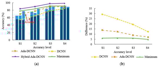
Figure 11.
The comparison of the hybrid Ada-DCNN, Ada-DCNN, and DCNN in 4 accuracy levels: (a) The accuracy of hybrid Ada-DCNN, Ada-DCNN, and DCNN; (b) The comparison of the hybrid Ada-DCNN, Ada-DCNN, and DCNN in 4 accuracy levels.
5.3. Robustness of the Hybrid Ada-DCNN
Based on studies in Section 5.1 and Section 5.2, the hybrid Ada-DCNN has been proved to have the best in fault diagnosis compared to Ada-DCNN and DCNN. In the construction of DCNNs, there are some situations where one or several DCNN(s) have difficulty achieving a satisfying accuracy (e.g., above 70%) for effective extraction of features. How much impact will it generate on the performance of hybrid Ada-DCNN in such situations?
In this part, we investigate the robustness of the hybrid Ada-DCNN by dropping the accuracy of several DCNNs to a low level and estimate the corresponding performance of the hybrid Ada-DCNN. For this purpose, the best performance (97.70%) corresponding to [S4, S4, S4] in Table 7 is used as a reference, and three schemes are adopted, where one, two, and three DCNNs are chosen for dropping, respectively, to estimate the robustness of the hybrid Ada-DCNN.
Table 8 presents the changes under each scheme and the corresponding accuracy, reduction part of the Hybrid Ada-DCNN, Ada-DCNNs, and DCNNs. Figure 12 shows more details of the reductions before and after dropping.
Table 8.
Performance of the hybrid Ada-DCNN, Ada-DCNNs, and DCNNs under different schemes (“/” represents no change).
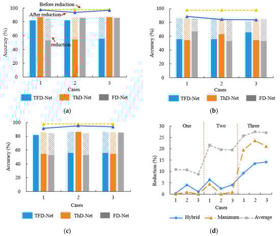
Figure 12.
The accuracy changes of the hybrid Ada-DCNN, Ada-DCNNs, and DCNNs under different schemes: (a) Changes in accuracy with one DCNN dropped; (b) Changes in accuracy with two DCNNs dropped; (c) Changes in accuracy with three DCNNs dropped; (d) Reductions from the reference accuracy under each scheme.
According to the results, the accuracy reduction of hybrid Ada-DCNN increases with the average dropped amplitude of DCNNs increasing. However, the average reduction of hybrid Ada-DCNN is 1.83%, 4.31%, and 12.29% in absolute terms separately for schemes 1–3, which are much lower than those corresponding to 10.11%, 20.21%, and 26.75% of DCNNs, respectively. The accuracy of hybrid Ada-DCNN is declined within an absolute value of 5% when one and two DCNNs dropped. The largest reduction is 12.29%, which occurs when all the DCNNs dropped, which generally does not happen. Additionally, it is found in Figure 12d that the accuracy reduction of hybrid Ada-DCNN is closely correlated with the change of maximal accuracy of DCNNs, which validates the conclusion obtained in Section 5.2 again.
The results above prove good robustness of the proposed hybrid fault diagnosis scheme.
6. Conclusions
In this paper, we propose a scheme that combined diverse CNN learners and AdaBoost tree-based ensemble classifier. The information of raw signals in the time domain, frequency domain, and time-frequency domain are employed in form of 2D images for diagnosis. Differently, samples are constructed separately and contribute to fault diagnosis simultaneously, which eliminates the situation that only one domain is focused or an elaborate feature integration across different domains must be determined in traditional vibration-based fault diagnosis, thus providing more freedom for the sample construction where each type of sample can concentrate on one aspect of the signal.
An example based on the CWRU datasets is illustrated to prove the superiority of the proposed scheme by two steps: (1) comparing the performance between DCNN and Ada-DCNN (single DCNN embedded), and (2) comparing the performance between Ada-DCNN and hybrid Ada-DCNN (multi-DCNNs embedded). Both comparisons above are carried out under accuracy levels growing from S1 to S4. The results show that the diagnosis accuracy is averagely improved by an absolute value of 15.37%, 12.29%, 10.40%, and 5.14% from S1 to S4 by using Ada-DCNN instead of DCNN, and 29.26%, 24.59%, 18.68%, and 12.95% by using hybrid Ada-DCNN. Besides, robustness of the proposed hybrid Ada-DCNN is also investigated by dropping the performance of one or more DCNNs embedded. It presents a reduction of only 1.83%, 4.31%, and 12.29% of hybrid Ada-DCNN versus the average drop of 10.11%, 20.21%, and 26.75% of one, two, and three DCNNs, respectively.
According to the results above, a hybrid Ada-DCNN is recommended for use in practical vibration-based fault diagnosis instead of traditional single DCNN method. The example in this paper has provided a specific way for using the proposed scheme to diagnose where the signal preprocessing and image sample construction methods can also be applied in other vibration-based analysis.
Author Contributions
Conceptualization, Q.Y. and B.Z.; methodology, B.Z.; software, H.Z.; validation, B.Z., H.Z.; formal analysis, Q.Y.; investigation, B.Z.; resources, H.Z.; data curation, H.Z.; writing—original draft preparation, B.Z.; writing—review and editing, B.Z., H.Z., and Q.Y.; visualization, H.Z.; supervision, Q.Y.; project administration, Q.Y.; funding acquisition, Q.Y. All authors have read and agreed to the published version of the manuscript.
Funding
This research was funded by the National Nature Science Foundation of China, grant number 11872289, and the Key Project of Natural Science Foundation of Xi’an Jiao Tong University, grant number ZRZD2017025. And the APC was funded by the National Nature Science Foundation of China, grant number 11872289.
Acknowledgments
The authors would like to thank the Case Western Reserve University Bearing Data Center for providing the data for this study.
Conflicts of Interest
The authors declare no conflicts of interest.
Data and Method Sharing Statement
The dataset and DLM used and analyzed during the current study are available from the corresponding authors upon reasonable request.
Nomenclature
| DCNN | Deep convolutional neural network |
| 2D | Two-dimensional |
| WT | Wavelet transform |
| DWT | Discrete wavelet transform |
| CWT | Continuous wavelet transform |
| WPT | Wavelet Packet Transform |
| HT | Hilbert Transform |
| Ada-DCNN | Single DCNN with AdaBoost tree-based ensemble classifier |
| Hybrid Ada-DCNN | Multi-DCNNs with AdaBoost tree-based ensemble classifier |
| FC | Fully connected layer |
| d | Bearing inside diameter |
| D | Bearing outside diameter |
| f0 | Running frequency |
| DB | Ball diameter of bearing |
| B | Bearing thickness |
| Dp | Bearing pitch diameter |
| IR | Bearing inner ring |
| OR | Bearing outer ring |
| RE | Rolling element |
| NC | Normal condition |
| DE | Drive end |
| FE | Fan end |
| RPM | Revolutions per minute |
| FD | Frequency domain |
| TFD | Time-frequency domain |
| ThD | Three domains |
| FD-Net | DCNN based on FD samples |
| TFD-Net | DCNN based on TFD samples |
| ThD-Net | DCNN based on ThD samples |
| Si | Accuracy of the ith level |
| Maximum | Maximal accuracy of DCNNs |
| Average | Average accuracy of DCNNs |
References
- Loparo, K.A.; Adams, M.L.; Lin, W.; Abdel-Magied, M.F.; Afshari, N. Fault detection and diagnosis of rotating machinery. IEEE Trans. Ind. Electron. 2000, 47, 1005–1014. [Google Scholar] [CrossRef]
- Liu, X.; Bo, L.; He, X.; Veidt, M. Application of correlation matching for automatic bearing fault diagnosis. J. Sound. Vib. 2012, 331, 5838–5852. [Google Scholar] [CrossRef]
- Jalan, A.K.; Mohanty, A.R. Model based fault diagnosis of a rotor–bearing system for misalignment and unbalance under steady-state condition. J. Sound. Vib. 2009, 327, 604–622. [Google Scholar] [CrossRef]
- Yi, J.; Liu, H.; Wang, F.; Li, M.; Jing, M. The resonance effect induced by the variable compliance vibration for an elastic rotor supported by roller bearings. J. Multi Body Dyn. 2014, 228, 380–387. [Google Scholar] [CrossRef]
- Goepfert, O.; Ampuero, J.; Pahud, P.; Boving, H.J. Surface roughness evolution of ball bearing components. Tribol. Trans. 2000, 43, 275–280. [Google Scholar] [CrossRef]
- Lynagh, N.; Rahnejat, H.; Ebrahimi, M.; Aini, R. Bearing induced vibration in precision high speed routing spindles. Int. J. Mach. Tool Manu. 2000, 40, 561–577. [Google Scholar] [CrossRef]
- Wardle, F.P. Vibration forces produced by waviness of the rolling surfaces of thrust loaded ball bearings part 1: Theory. J. Mech. Eng. Sci. 1988, 202, 305–312. [Google Scholar] [CrossRef]
- Li, W.; Qiu, M.Q.; Zhu, Z.C.; Jiang, F.; Zhou, G. Fault diagnosis of rolling element bearings with a spectrum searching method. Meas. Sci. Technol. 2017, 28, 1–16. [Google Scholar] [CrossRef]
- Zhao, R.; Wang, D.; Yan, R.; Mao, K.; Shen, F.; Wang, J. Machine health monitoring using local feature-based gated recurrent unit networks. IEEE Trans. Ind. Electron. 2018, 65, 1539–1548. [Google Scholar] [CrossRef]
- Razavi-Far, R.; Farajzadeh-Zanjani, M.; Saif, M. An integrated class-imbalance learning scheme for diagnosing bearing defects in induction motors. IEEE Trans. Industr. Inform. 2017, 13, 2758–2769. [Google Scholar] [CrossRef]
- Song, L.; Wang, H.; Chen, P. Vibration-based intelligent fault diagnosis for roller bearings in low-speed rotating machinery. IEEE Trans. Instrum. Meas. 2018, 67, 1–13. [Google Scholar] [CrossRef]
- Liu, Y.K.; Guo, L.W.; Wang, Q.X.; An, G.; Guo, M.; Lian, H. Application to induction motor faults diagnosis of the amplitude recovery method combined with FFT. Mech Syst Signal Pr 2010, 24, 2961–2971. [Google Scholar] [CrossRef]
- Keskes, H.; Braham, A. Recursive undecimated wavelet packet transform and DAG SVM for induction motor diagnosis. IEEE Trans. Industr. Inform. 2015, 11, 1059–1066. [Google Scholar] [CrossRef]
- Li, Y.; Xu, M.; Liang, X.; Huang, W. Application of Bandwidth EMD and Adaptive Multi-Scale Morphology Analysis for Incipient Fault Diagnosis of Rolling Bearings. IEEE Trans. Ind. Electron. 2017, 64, 6506–6517. [Google Scholar] [CrossRef]
- Tian, Y.; Ma, J.; Lu, C.; Wang, Z. Rolling bearing fault diagnosis under variable conditions using LMD-SVD and extreme learning machine. Mech. Mach. Theory 2015, 90, 175–186. [Google Scholar] [CrossRef]
- Rai, V.K.; Mohanty, A.R. Bearing fault diagnosis using FFT of intrinsic mode functions in Hilbert–Huang transform. Mech. Syst. Signal Process. 2007, 21, 2607–2615. [Google Scholar] [CrossRef]
- Gao, H.Z.; Liang, L.; Chen, X.G.; Xu, G. Feature extraction and recognition for rolling element bearing fault utilizing short-time Fourier transform and non-negative matrix factorization. Chin. J. Mech. Eng. 2015, 28, 96–105. [Google Scholar] [CrossRef]
- Ali, J.B.; Fnaiech, N.; Saidi, L.; Chebel-Morello, B.; Fnaiech, F. Application of empirical mode decomposition and artificial neural network for automatic bearing fault diagnosis based on vibration signals. Appl. Acoust. 2015, 89, 16–27. [Google Scholar]
- Guo, W.; Peter, W.T. A novel signal compression method based on optimal ensemble empirical mode decomposition for bearing vibration signals. J. Sound Vib. 2013, 332, 423–441. [Google Scholar] [CrossRef]
- Vafaei, S.; Rahnejat, H. Indicated repeatable runout with wavelet decomposition (IRR-WD) for effective determination of bearing-induced vibration. J. Sound Vib. 2003, 260, 67–82. [Google Scholar] [CrossRef]
- Huo, Z.; Zhang, Y.; Francq, P.; Shu, L.; Huang, J. Incipient fault diagnosis of roller bearing using optimized wavelet transform based multi-speed vibration signatures. IEEE Access 2017, 5, 19442–19456. [Google Scholar] [CrossRef]
- Wang, P.; Yan, R.; Gao, R.X. Virtualization and deep recognition for system fault classification. J. Manuf. Syst. 2017, 44, 310–316. [Google Scholar]
- Islam, M.M.M.; Kim, J.M. Automated bearing fault diagnosis scheme using 2D representation of wavelet packet transform and deep convolutional neural network. Comput. Ind. 2019, 106, 142–153. [Google Scholar] [CrossRef]
- Wang, D.; Tse, P.W.; Tsui, K.L. An enhanced kurtogram method for fault diagnosis of rolling element bearings. Mech. Syst. Signal Process. 2013, 35, 176–199. [Google Scholar] [CrossRef]
- Browne, M.; Ghidary, S.S. Convolutional Neural Networks for Image Processing: An Application in Robot Vision, Australasian Joint Conference on Artificial Intelligence; Springer: Berlin/Heidelberg, Germany, 2003; pp. 641–652. [Google Scholar]
- Mayya, V.; Pai, R.M.; Manohara Pai, M.M. Automatic facial expression recognition using DCNN. Procedia Comput. Sci. 2016, 93, 453–461. [Google Scholar] [CrossRef]
- Jing, L.; Wang, T.; Zhao, M.; Wang, P. An adaptive multi-sensor data fusion method based on deep convolutional neural networks for fault diagnosis of planetary gearbox. Sensors 2017, 17, 414. [Google Scholar] [CrossRef]
- Huang, R.Y.; Xiao, Y.; Li, W. Deep decoupling convolutional neural network for intelligent compound fault diagnosis. IEEE Access 2018, 7, 1848–1858. [Google Scholar] [CrossRef]
- Qiu, G.Q.; Gu, Y.K.; Cai, Q. A deep convolutional neural networks model for intelligent fault diagnosis of a gearbox under different operational conditions. Measurement 2019, 145, 94–107. [Google Scholar] [CrossRef]
- Razavi-Far, R.; Hallaji, E.; Farajzadeh-Zanjani, M.; Saif, M.; Kia, S.H.; Henao, H.; Capolino, G.A. Information Fusion and Semi-Supervised Deep Learning Scheme for Diagnosing Gear Faults in Induction Machine Systems. IEEE Trans. Ind. Electron. 2011, 66, 6331–6342. [Google Scholar]
- Zhao, R.; Yan, R.; Chen, Z.; Mao, K.; Wang, P.; Gao, R.X. Deep learning and its applications to machine health monitoring. Mech. Syst. Signal Process. 2019, 115, 213–237. [Google Scholar] [CrossRef]
- Zhang, B.H.; Qi, S.L.; Monkam, P.; Li, C.; Yang, F.; Yao, Y.D.; Qian, W. Ensemble Learners of Multiple Deep CNNs for Pulmonary Nodules Classification Using CT Images. IEEE Access 2019, 7, 110358–110371. [Google Scholar] [CrossRef]
- Li, S.B.; Liu, G.K.; Tang, X.H.; Lu, J.; Hu, J. An ensemble Deep Convolutional Neural Network model with improved D-S evidence fusion for bearing fault diagnosis. Sensors 2017, 17, 1729. [Google Scholar] [CrossRef] [PubMed]
- Xu, G.W.; Liu, M.; Jiang, Z.F.; Söffker, D.; Shen, W. Bearing fault diagnosis method based on Deep Convolutional Neural Network and Random Forest Ensemble learning. Sensors 2019, 19, 1088. [Google Scholar] [CrossRef] [PubMed]
- Borghesani, P.; Ricci, R.; Chatterton, S.; Pennacchi, P. A new procedure for using envelope analysis for rolling element bearing diagnostics in variable operating conditions. Mech. Syst. Signal Process. 2013, 38, 23–35. [Google Scholar] [CrossRef]
- Bo, M.; Qiang, W.; Chun, X. Envelope analysis based on Hilbert transformation and its application in ball bearing fault diagnosis. J. Beijing Univ. Chem. Technol. 2004, 31, 95–97. [Google Scholar]
- Freund, Y.; Schapire, R.E. Experiments with a new boosting algorithm. In Proceedings of the Thirteenth International Conference on Machine Learning, San Francisco, CA, USA, 3–6 July 1996; pp. 148–156. [Google Scholar]
- Li, X.; Wang, L.; Sung, E. A study of AdaBoost with SVM based weak learners. In Proceedings of the International Joint Conference on neural networks, Montreal, QC, Canada, 31 July–4 August 2005; pp. 196–201. [Google Scholar]
- Schwenk, H.; Bengio, Y. Boosting Neural Networks. Neural Comput. 2000, 12, 1869–1887. [Google Scholar] [CrossRef]
- Dietterich, T.G. An Experimental comparison of three methods for constructing ensembles of decision trees: Bagging, boosting, and randomization. Mach. Learn. 2000, 40, 139–157. [Google Scholar] [CrossRef]
- Wade, A.S.; Robert, B.R. Rolling element bearing diagnostics using the Case Western Reserve University data: A benchmark study. Mech. Syst. Signal Process. 2015, 64–65, 100–131. [Google Scholar]
- Gousseau, W.; Antoni, J.; Girardin, F.; Griffaton, J. Analysis of the rolling element bearing data set of the center for intelligent maintenance systems of the University of Cincinnati; CM2016: Charenton, France, 2016. [Google Scholar]
- Case Western Reserve University Bearing Data Center Website. Available online: http://csegroups.case.edu/bearingdatacenter/home (accessed on 5 March 2020).
© 2020 by the authors. Licensee MDPI, Basel, Switzerland. This article is an open access article distributed under the terms and conditions of the Creative Commons Attribution (CC BY) license (http://creativecommons.org/licenses/by/4.0/).