Numerical Investigation of Locating and Identifying Pipeline Reflectors Based on Guided-Wave Circumferential Scanning and Phase Characteristics

Abstract

The methodology based on reflected guided-wave by a reflector associated with an increase or a decrease in the cross-sectional area has the challenge of determining their location and identity. This paper presents a numerical investigation of a method for locating and identifying the reflector based on guided-wave circumferential scanning and phase characteristics. To determine the axial and circumferential positions of the reflector within the pipeline, the procedures of the guided wave-based circumferential scanning were presented, including data preprocessing, median filter, image smoothing and binary processing. Through theoretical analysis, we obtained the phase relationship between the guided-wave excitation signal and reflection signals generated by a reflector, such as corrosion, crack, weld and support, which caused the change in the cross-sectional area. Consequently, an algorithm based on the phase characteristics was proposed to determine the change and type of reflector. The spatial distances were calculated between the guided wave excitation signals with different phases and the concerned reflection signals, subsequently identifying the change and type of the reflector by comparing the distance values. An identification index named the reliable index for the character of the reflector (RICR) was defined to evaluate the reliability of the predicted results. Numerical and finite element simulation validations of the proposed method were performed. It has been found that if RICR was larger than 1.05, the results predicting the reflector type were reliable. The proposed method was found to be superior relative to the conventional correlation coefficient method according to the numerical results. Finally, the simulation results demonstrated that the proposed method could be potentially applied for locating and identifying reflectors in pipelines.

1. Introduction

Employing ultrasonic-guided waves is one of the most commonly used techniques for non-destructive evaluation (NDE) and structural health monitoring (SHM) of the oil, gas, chemical and petrochemical industries, due to its key advantages such as rapid screening with 100% cross-section coverage, long-distance and large-range diagnostic capability and high detection efficiency [1,2,3,4,5]. A guided wave is of multiple modes which are sensitive to different types of acoustic reflectors as their acoustic impedances are changed. The acoustic impedance of a reflector depends solely on their area within a cross-section of a uniform pipe-material with the same density and velocity of the wave. Therefore, when a short pulse of the guided wave is launched along a structure, a reflected signal will be generated by the reflector which is associated with the change in the cross-section area. As shown in Figure 1, the change can be either an increase or a decrease and can be caused by corrosions, cracks, welds or supports in a pipeline. The reflected wave contains abundant information about the tested reflector, which can then be utilized to locate and identify it.

Reflectors associated with changes like an increase or a decrease in the cross-sectional areas exist in most structures. In the past few years, in order to understand the relationships between the geometrical properties of the acoustic reflector and the guided-wave propagation characteristics, many researchers have contributed to investigating the scattering and reflection from various reflectors, such as cracks, notches, welds, supports and holes [6,7,8,9,10,11,12,13]. Because it represents an important role in guided-wave inspection, the considerable amount of aforementioned work has mainly focused on the direct problem of analyzing responses such as propagation, reflection and conversion coming from different known reflectors, while more attention needs to be paid to the inverse problem of automatically diagnosing and distinguishing the type of the unknown reflectors by their responses. By following this direction of research, Zhang [6] recently studied the scattering of torsional flexural guided waves from different defects in hollow cylinders and proposed a novel classification and characterization method for defects in a pipe, which can be used to preliminarily categorize circular holes and crack-like defects. Muñoz [14] proposed a novel signal processing approach which is able to automatically identify notches in pipelines in short distances.

In practical applications, there is an urgent need to develop a quick and reliable method for identifying and locating a reflector. This is due to the fact that reflectors causing an increase in the cross-sectional area, such as supports, flanges and butt welds, usually belong to geometric features; while reflectors which decrease it, such as corrosion and cracks, usually belong to defect features which need to be detected and treated early to minimize their consequences. If the former and the latter cannot be correctly identified and distinguished, it will usually lead to false positives or negatives being recorded during a guided-wave inspection. Efficient methods based on guided-wave circumferential scanning for identifying the reflector have not been proposed yet. Therefore, a study for identifying and locating pipeline reflectors based on guided-wave circumferential scanning and phase characteristics was carried out in this pager. The paper is organized as follows: Section 2 introduces the principle of guided-wave circumferential scanning technique for a pipe. Theoretical analysis to find out the phase characteristics of the guided wave reflected from a reflector is given in Section 3. Section 4 presents the procedures of the proposed method and algorithm. The proposed method is then applied to numerical and simulation signals to validate its validity and robustness in Section 5 followed by conclusions in Section 6.

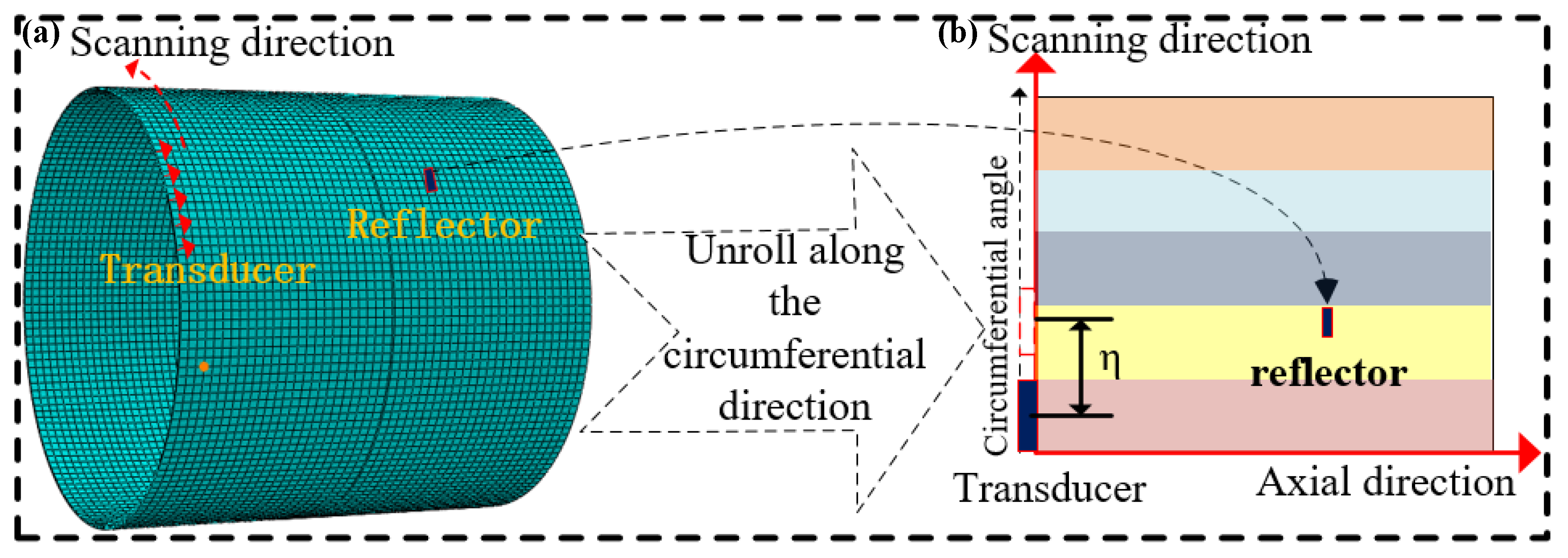
2. Principle of Guided-Wave Circumferential Scanning Technique for a Pipe

The guided-wave circumferential scanning technique can obtain two-dimensional (2D) information such as the circumferential size and distribution of a reflector over the conventional A-scan, meaning that the location and extent of the reflector can be then presented on a map. Compared with the imaging technique using the guided-wave multi-channel phased array technique [15,16], the circumferential scanning technique with fewer circumferential transducers is more flexible and easier to operate [17]. As illustrated in Figure 2a,b, a pipe with a reflector is unwrapped by moving the transducer with a given step η along the circumferential direction while the scanned 2D circumferential scanning image of the reflector is reconstructed.

In this work, firstly, we can discriminate the geometric features like a flange, pipe end or girth weld from the defect features by utilizing the circumferential scanning technique illustrated in Figure 3a–f, as these reflecting features are continuous from bottom to top in the 2D circumferential scanned image shown in Figure 3e,f due to their axisymmetric geometry. Compared with Figure 3c,d, Figure 3e,f contain the circumferential distribution of the reflectors. However, it is difficult to judge whether a reflector like a support is a defect feature such as a corrosion, since both the support and the corrosion are both discontinuous from the bottom to the top in the circumferential scanned image as a consequence of them being usually located within a small circumferential range (angle), as illustrated in Figure 2b. This phenomenon introduces the serious possibility of false positives or negatives, such as a support being incorrectly identified as a defect.

For the above problem, in order to further discriminate whether a reflector is a defect feature decreasing the cross-sectional area or a geometric feature increasing it, a novel method based on the phase characteristics is proposed. A further detailed discussion about its algorithm is covered in Section 4.

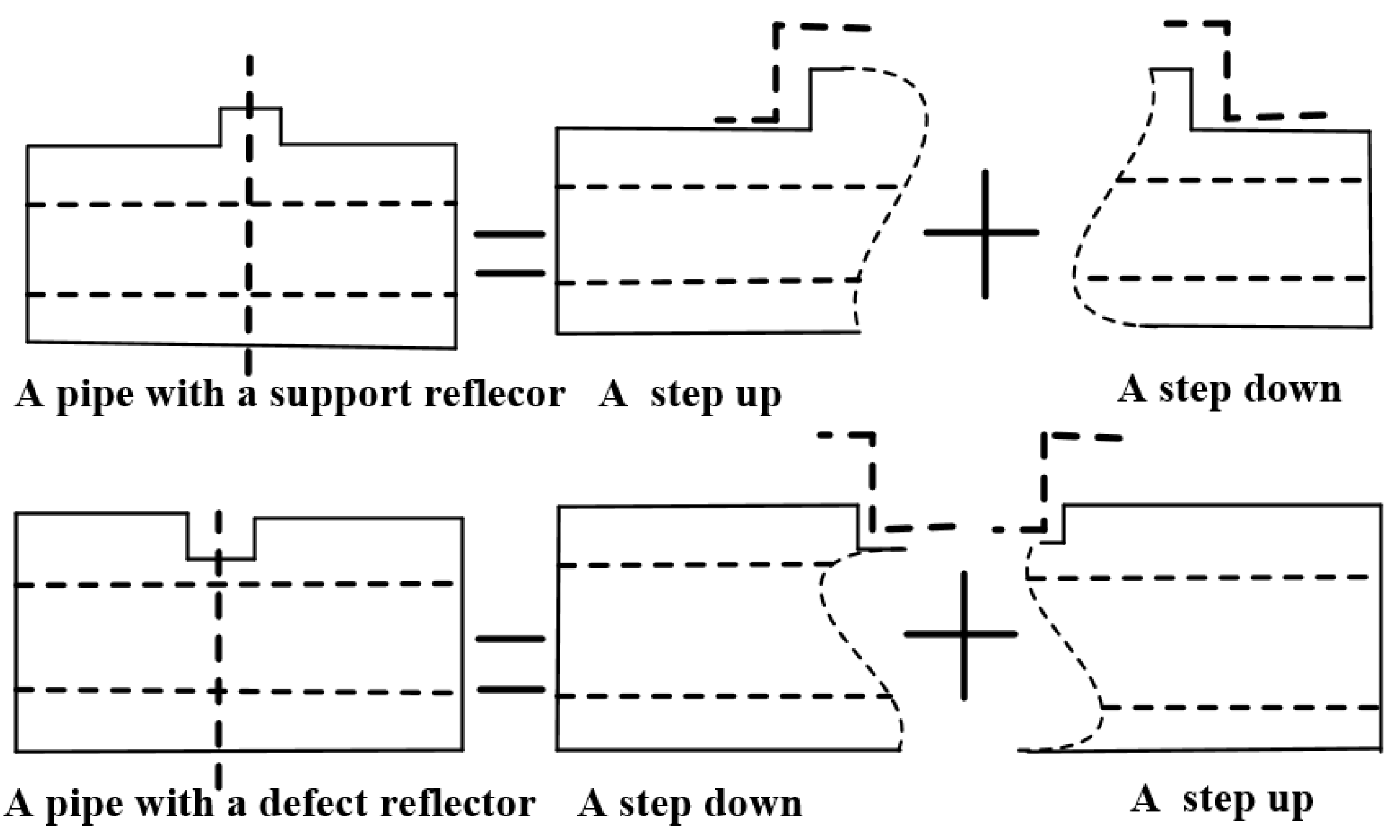
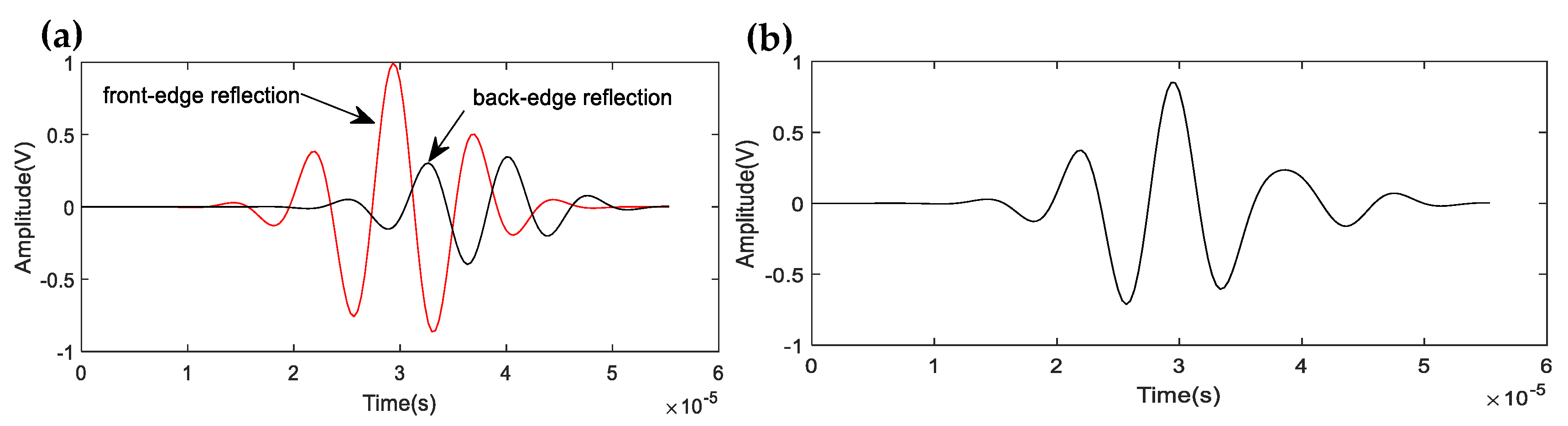
3. Phase Characteristics of the Guided Wave Reflected from a Reflector

Based on reference [18], the guided waves propagating in the axial direction in pipes involve torsional waves T(N,m) and longitudinal waves L(N,m), where the integer N denotes the circumferential order and m represents the group order of a mode. Because the fundamental torsional guided wave mode T(0,1) has the attracting characteristics of no dispersion, low probability of mode conversion, uniform wave-structures in the thickness direction and no response to liquids that may exist at the pipe surface, T(0,1) is most commonly used for pipe inspection [19] and was selected in this work for investigation. This paper considers a case in which T(0,1) is incident on a reflector and only T(0,1) could potentially propagate in the pipe (T(0,1) excited at a frequency lower than the T(0,2) cut-off frequency). The presence of the reflector causes guided-wave scattering, consequent reflection and transmission of the incident wave (IN), as shown in Figure 4a. The chosen axial direction of the pipe was the x-axis, and the coordinate origin is located at the reflector. The acoustic pressures p_i, p_r and p_t of IN, reflected wave (RE) and transmission wave (TR) are defined as the following form of simple harmonic waves respectively:

$$\begin{array}{c}{p}_i=P_{i0}\exp (i(\omega t-kx)) (\mathrm{propagation}\mathrm{along}\mathrm{the}\mathrm{positive}\mathrm{direction}\mathrm{of}\mathrm{the}\mathrm{x-axis})\\ p_r=P_{r0}\exp (i(\omega t+kx))(\mathrm{propagation}\mathrm{along}\mathrm{the}\mathrm{negtive}\mathrm{direction}\mathrm{of}\mathrm{the}\mathrm{x-axis})\\ p_t=P_{t0}\exp (i(\omega t-kx))\end{array}$$

(1)

where P_i0, P_r0 and P_t0 are the maximum acoustic pressures; k and ω are the wavenumber and angular frequency, respectively. According to the relationship between acoustic pressure and acoustic impedance [20], the corresponding particle velocities can be depicted as:

$$\begin{array}{c}{v}_i=\raisebox{1ex}{$P_{i0}$}\!\left/ \!\raisebox{-1ex}{$\rho c$}\right.\exp (i(\omega t-kx))\\ v_r=-\raisebox{1ex}{$P_{r0}$}\!\left/ \!\raisebox{-1ex}{$\rho c$}\right.\exp (i(\omega t+kx))\\ v_t=\raisebox{1ex}{$P_{t0}$}\!\left/ \!\raisebox{-1ex}{$\rho c$}\right.\exp (i(\omega t-kx))\end{array}$$

(2)

where ρ is the density of the pipe; c is guided wave velocity. Considering that the boundary conditions should be continuous at the reflector, the acoustic pressure and volume velocity are continuous:

$$\begin{array}{c}{p}_i(0)+p_r(0)=p_t(0)\\ {\delta }_1\times (v_i(0)+v_r(0))={\delta }_2\times v_t(0)\end{array}$$

(3)

where δ₁ and δ₂ are the cross-sectional areas of the pipe and the reflector respectively. Substituting Equations (1) and (2) into Equation (3), we obtain the relationship:

$${\delta }_1\times (P_{i0}-P_{r0})={\delta }_2\times (P_{i0}+P_{r0})$$

(4)

Further assuming ξ = $\raisebox{1ex}{${\delta }_1$}\!\left/ \!\raisebox{-1ex}{${\delta }_2$}\right.$, the reflection coefficient (RC) is obtained according to Equation (4):

$$\mathrm{RC}=\raisebox{1ex}{$P_{r0}$}\!\left/ \!\raisebox{-1ex}{$P_{i0}$}\right.=\frac{\xi -1}{\xi +1}{=\mathrm{R}}_{\mathrm{e}}{+\mathrm{jI}}_{\mathrm{m}}$$

(5)

where R_e and I_m are the real and imaginary parts of the RC, which are illustrated in the complex plane in Figure 4b.

Therefore, the impedance angle and module of RC shown in Figure 4b are calculated respectively as:

$$\begin{array}{l}\left|\theta \right|=\left|\arctan ({\mathrm{I}}_{\mathrm{m}}/{\mathrm{R}}_{\mathrm{e}})\right|=\left|{\theta }_{\mathrm{Re}}-{\theta }_{\mathrm{In}}\right|\\ \left|\mathrm{RC}\right|=\sqrt{{\mathrm{I}}_{\mathrm{m}}{}^2{+\mathrm{R}}_{\mathrm{e}}{}^2}\end{array}$$

(6)

where θ_In and θ_Re are the phases of the incident wave and the reflection wave respectively. From Equations (5) and (6), the phase characteristics of the guided wave reflected from a reflector can be obtained as follows:

(a)

If δ₁ < δ₂, namely RC < 0, so the phase shift $\left|\theta \right|=\left|\arctan ({\mathrm{I}}_{\mathrm{m}}/{\mathrm{R}}_{\mathrm{e}})\right|=\left|{\theta }_{\mathrm{Re}}-{\theta }_{\mathrm{In}}\right|=(2\mathrm{k}-1)\pi$, k = 1, 2, …, n.

(b)

If δ₁ > δ₂, namely RC > 0, so the phase shift $\left|\theta \right|=\left|\arctan ({\mathrm{I}}_{\mathrm{m}}/{\mathrm{R}}_{\mathrm{e}})\right|=\left|{\theta }_{\mathrm{Re}}-{\theta }_{\mathrm{In}}\right|=2\mathrm{k}\pi$, k = 0, 1, …, n.

(c)

If δ₁ = δ₂, RC = 0, this indicates there is no reflector in the pipeline.

(d)

If ${\delta }_1\gg {\delta }_2$, this means almost all of the incident wave is reflected back.

A defect or support reflector can be decomposed into a step down (front-edge of the reflector, namely δ₁ > δ₂) and a step up (back-edge of the reflector, namely δ₁ < δ₂), as shown in Figure 5. Thus, for a defect reflector, the incident wave is in the same phase with the reflection wave generated from the front-edge of the reflector; while the wave reflected from the back-edge of the reflector is in the opposite phase with the incident wave, according to the above conclusions.

4. Proposed Method Based on the Circumferential Scanning and Phase Characteristics

The guided-wave signals reflected from a reflector are the overlapping results of the reflection components from the step down and the step up. Figure 6 illustrates the wave propagation paths corresponding to the individual signals in a pipe with a defect reflector, where S_i(t) and S_r(t) are the incident signal and its reflection signal, respectively.

As shown in Figure 6, the RCs and transmission coefficients (TC) at the front- and back-edge of the reflector are respectively defined as: reflection coefficient RC₁ = RE₁/S_i(t), transmission coefficient TC₁ = TR₁/S_i(t), reflection coefficient RC₂ = RE₂/TR₁, transmission coefficient TC₂ = TR₂/TR₁, reflection coefficient RC₃ = RE₃/RE₂, transmission coefficient TC₃ = TR₃/RE₂, and {RC₁, TC₁, RC₂, TC₂, RC₃, TC₃ } ∈ [0, 1]. The reflection signals received from the reflector, S_r(t), may be modelled as:

S_r(t) = RE₁+ TR₃ + Ψ(t) = RC₁ × S_i(t) + TC₁ × RC₂ × TC₃ × S_i(t − t₀) + Ψ(t) =
S_r1(t) + S_r2(t − t₀) + Ψ(t), 0 < t < T

(7)

where S_r1(t) and S_r2(t) represent the reflection responses from the front- and back- edge of the reflector, Ψ(t) corresponds to the uncorrelated noise, T is the observation time, and t₀ is the time delay, estimated by the axial length of the reflector and wave velocity. Reflections from the reflector cause different degrees of signal decay, in a similar way to the acoustic energy marked in Figure 6. Obviously, S_r1(t) > S_r2(t), which means that S_r1(t) generated from the front-edge of the reflector is the main component of S_r(t). Therefore, S_r1(t) includes the main information of the overlapping signals and determines the characteristics of the reflector (shape and size), as illustrated in Figure 7. Consequently, only the change of the front-edge (a step down or a step up) of the reflector needs to be identified by the phase characteristics described in Section 3, then the type and shape of the reflector (geometric or defect feature) can be determined.

Based on the above analysis, the method for locating and identifying the reflector in pipelines is proposed as follows. Firstly, a 2D image of the reflecting features in the pipe is reconstructed through the guided-wave circumferential scanning technique and image processing, and the axial and circumferential positions of the reflector are obtained. Secondly, to identify the change of the front-edge and further obtain the type of the reflector, the method based on phase characteristics is developed by calculating the spatial distances between S_i(t) and S_r(t). According to Equation (7), discrete signals S_i(n) and S_r(n) are obtained by sampling S_i(t) and S_r(t). Before calculating, the distances between S_i(n) and S_r(n), S_r(n) need to be preprocessed first to obtain the data matrix $Y_{M\times {\Gamma }_i}$ $=\left[\begin{array}{c}{s}_{r1}\\ s_{r2}\\ ⋮\\ s_{rM}\end{array}\right]=\left[\begin{array}{cccc}{s}_{r11}& s_{r12}& \cdots & s_{r1{\Gamma }_i}\\ s_{r21}& s_{r22}& \cdots & s_{r2{\Gamma }_i}\\ ⋮& ⋮& \cdots & ⋮\\ s_{rM1}& s_{rM2}& \cdots & s_{rM{\Gamma }_i}\end{array}\right]$ by applying a rectangular window function $w\left(n\right)=\{\begin{array}{c}1,0<n\le {\Gamma }_i\\ 0,otherwise\end{array}$ and an analysis step $\gamma \in [1,{\Gamma }_i]$, and $M=[\raisebox{1ex}{$({\Gamma }_r-{\Gamma }_i)$}\!\left/ \!\raisebox{-1ex}{$\gamma $}\right.+1],$ where $[\raisebox{1ex}{$({\Gamma }_r-{\Gamma }_i)$}\!\left/ \!\raisebox{-1ex}{$\gamma $}\right.+1]$ denotes the largest integer no more than $\raisebox{1ex}{$({\Gamma }_r-{\Gamma }_i)$}\!\left/ \!\raisebox{-1ex}{$\gamma $}\right.+1$, Γ_i and Γ_r are the dimensions of S_i(n) and S_r(n), respectively. We adopt the standard Euclidian distance to calculate the distance values $D(S_i,S_{ri})$ between $Y_{M\times {\Gamma }_i}$ and S_i(n), which is written as:

$$D(S_i,S_{ri})=\sqrt{{\displaystyle \sum _{j=1}^N{(\frac{s_i-s_{rij}}{{\tau }_i})}^2}}\in [0,\infty ),(\mathrm{i}=1,2,\dots ,\mathrm{M})$$

(8)

where ${\tau }_i$ is the standard deviation of S_ri(n). Similarly, the distance values $D(\overline{\overline{S_i}},S_{ri})$ are obtained according to Equation (8), where parameters of $\overline{\overline{S_i}}$ are the same as $S_i$ except that the phase is opposite. Then, the minimum values of D₁ = min{$D(S_i,S_{ri})$} and D₂ = min{$D(\overline{\overline{S_i}},S_{ri})$} are found. The change of the front-edge can be identified by comparing D₁ and D₂ and the shape of the reflector can be further determined. Finally, the results are updated into the 2D image using different colours.

To estimate the reliability and accuracy of the method, an identification index named the reliable index for the character of the reflector (RICR) is defined as:

$$RICR=10\ast \lg (\left|D_1-D_2\right|),RICR\in [-\infty ,\infty )$$

(9)

Based on the test results, it has been found that if RICR was larger than 1.05, the predicted results for the reflector type were reliable.

The main steps and workflow are described as:

Step 1: A 2D data matrix H_i*j is obtained by moving the transducer with a given step η along the circumferential direction of a pipe.

Step 2: The data matrix H_i*j is preprocessed to obtain upper envelopes, then an original 2D scanned image is constructed.

Step 3: The original image is further processed to obtain an enhanced 2D scanned binary image by using image enhancement, image smoothing and binary processing to improve the resolution and inspection accuracy. A reflector is then found, which is discontinuous from bottom to top in the 2D circumferential scanned image. Otherwise, the process returns to Step 1.

Step 4: The incident signal S_i with initial phase ${\theta }_{\mathrm{In}}$ is excited to generate T(0,1) mode guided wave, and S_r is received by sampling guided wave signals.

Step 5: A data matrix $Y_{M\times {\Gamma }_i}$ is constructed by gating S_r using the rectangular window function w(n) with analysis step size γ.

Step 6: Calculate standard Euclidian distance values $D(S_i,S_{ri})$ and $D(\overline{\overline{S_i}},S_{ri})$ to produce the spatial distance curves Ψ₁ and Ψ₂ respectively.

Step 7: D₁ = min{$D(S_i,S_{ri})$} and D₂ = min{$D(\overline{\overline{S_i}},S_{ri})$} are obtained from the above distance curves (except distance values of the incident wave and reflected waves from a pipe end or flange).

Step 8: If D₁ < D₂, the front-edge of the reflector is a step down, it indicates the reflector is a defect feature. Else if D₁ > D₂, the front-edge of the reflector is a step up, it means the reflector is a geometric feature (like a support or local weld). Otherwise, if D₁ = D₂, the compared result is deemed inconclusive.

Step 9: The value of the RICR is calculated using Equation (9), if RICR >1.05, the judgement is reliable.

Step 10: The enhanced 2D scanned binary image is updated with the result, the locations and type of the reflector are intuitively shown, as red indicates the reflector is a defect feature, and blue indicates the reflector is a geometric feature.

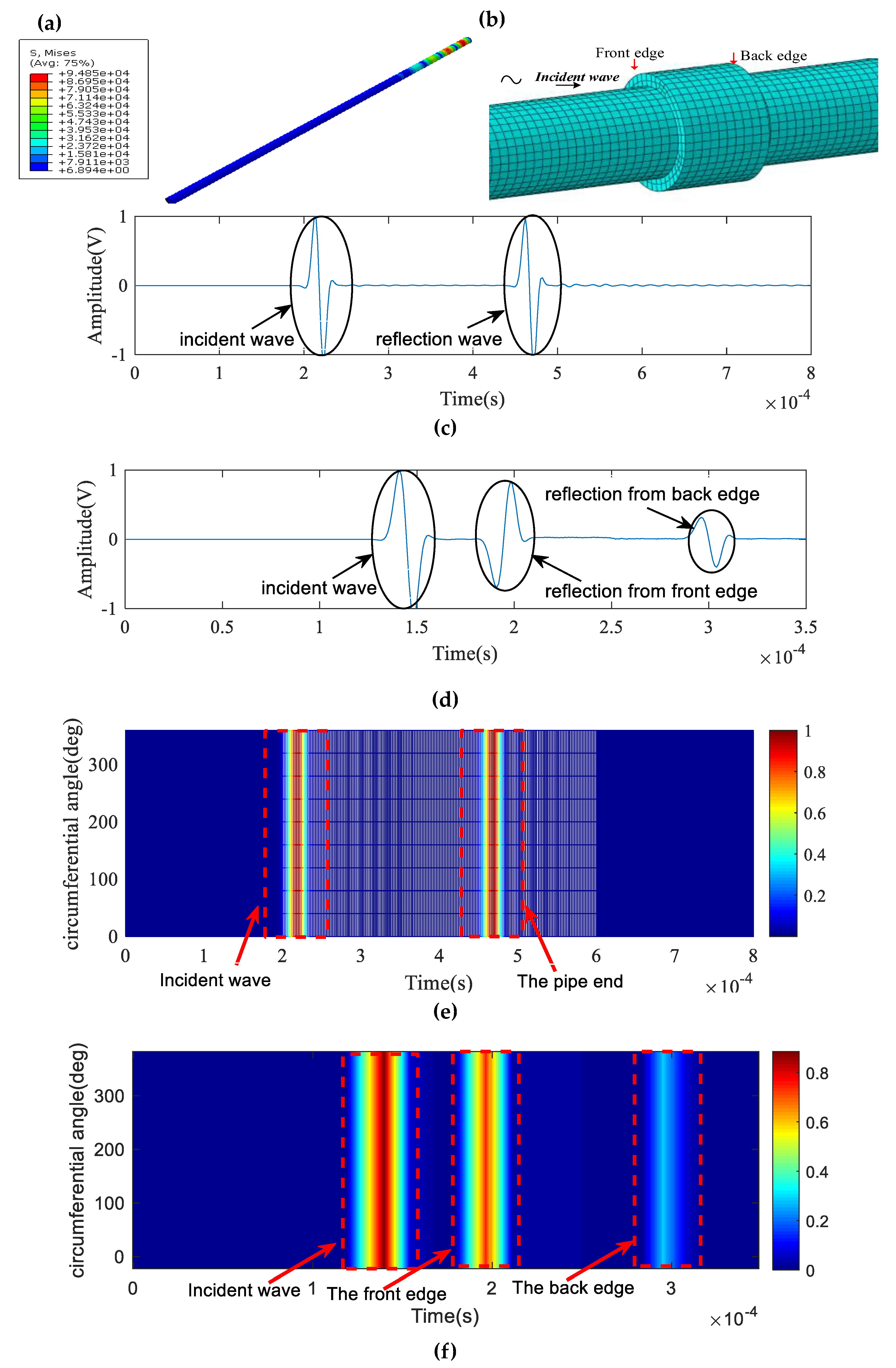
5. Numerical Simulation and Verification

In this section, the validity and robustness of the proposed method were investigated using numerical and simulated signals.

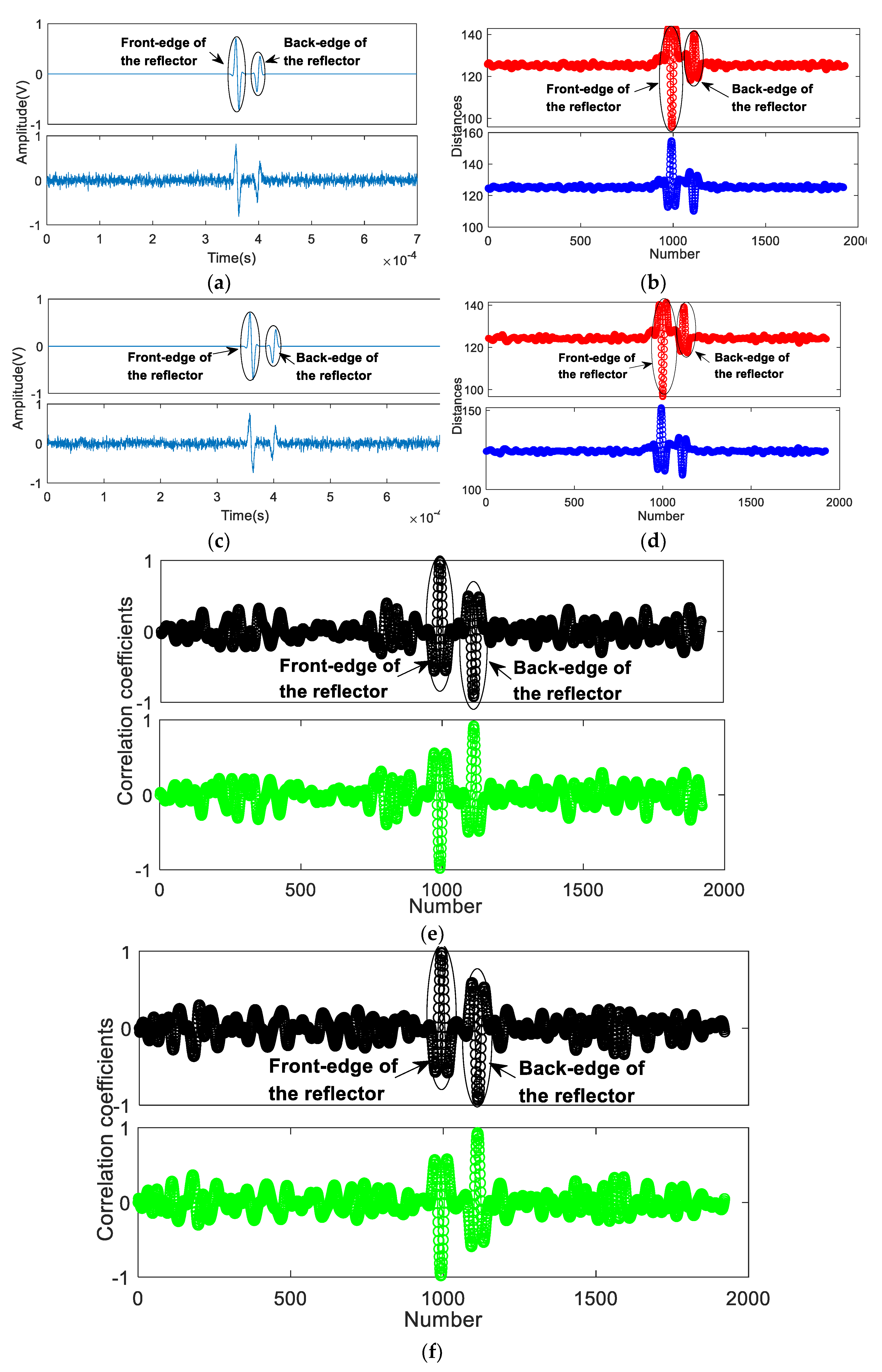
5.1. The Choice of the Incident (Excitation) Pulse Signal

The modulated Gaussian pulse was chosen (also known as the Gabor pulse) as the excitation pulse:

$$g(t)={\exp }^{-(t-\mu {)}^2/2{\sigma }^2}\cos \left(2\pi f_c(t-\mu )+\theta \right)$$

(10)

where σ, μ, f_c and θ represent the width of the pulse, time shift, centre frequency and phase, respectively. The main motivation for using Gabor pulse is that the Gabor waveform has the best time–frequency resolution [21].

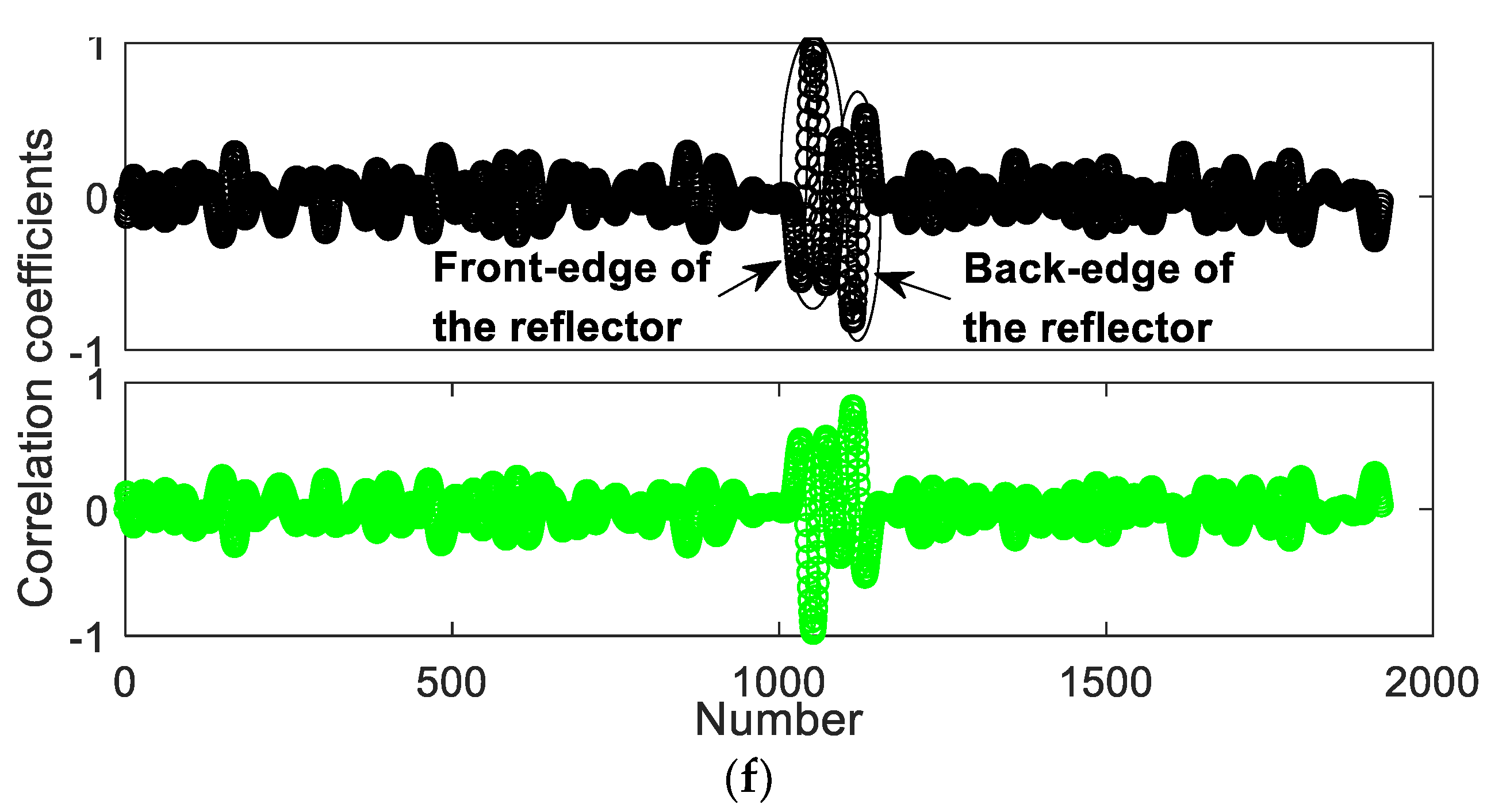
5.2. Numerical Investigation of the Proposed Method

For simplification, only Steps (5) to Step (9) in Section 3 are first checked for noise robustness in this section. Considering that the signal-to noise ratio (SNR) of the actual guided wave signal was poor, artificial noises were added into the numerical signals. A numerical guided wave signal $\widehat{x}(t)$ including two Gabor pulses $x_1(t)$, $x_2(t)$ and a random white noise ς(t), can be represented as:

$$\widehat{x}(t)=x(t)+\varsigma (t)=x_1(t)+x_2(t)+\varsigma (t)={\displaystyle \sum _{i=1}^2{A}_i{g}_i({\sigma }_i,u_i,f_{ci},{\theta }_i)(t)}+\varsigma (t)$$

(11)

where the SNR of $\widehat{x}(t)$ is defined as:

$$\mathrm{SNR}=10{\log }_{10}\frac{{\displaystyle \int {\left|x(t_i)\right|}^{2}dt}}{{\displaystyle \int {\left|n(t_i)\right|}^{2}dt}}(\mathrm{dB})$$

(12)

In the first case, the two Gabor pulses in $\widehat{x}(t)$ are not overlapped, which means that the axial length of the reflector is long enough. x₁(t) and x₂(t) represent the reflection signals from the front- and back-edge of a reflector, respectively, while the reflector is set as a defect. The sampling frequency is assumed to be f_s = 3000 kHz. The Gabor excitation pulse S_i is (σ, μ, θ_n, f_c) = (4 × 10⁻⁶ s, 2 × 10⁻⁶ s, π/2rad, 64 kHz). The specific parameters of the Gabor pulses g₁(t) and g₂(t) are tabulated in

Table 1. Parameters of Gabor pulses $x_1(t)$ and $x_2(t)$.

Pulses	Ai	σ	u (s)	fc (kHz)	θ (rad)
$x_1(t)$	1	4.0 × 10−6	3.6 × 10−4	64	π/2
$x_2(t)$	0.5	4.0 × 10−6	4.0 × 10−4	64	−π/2

.

After calculating in MATLAB, Figure 8 shows the numerical signals with different SNRs as well as comparisons of the results obtained from the proposed method and the correlation coefficient method. The observation time is T = 7 × 10⁻⁴ s. The dimensions of S_i(n) and ${\widehat{x}}_1(n)$ are Γ_i = 181 and Γ_r = 2101, respectively. The analysis step γ is equal to 1; therefore, the total number M = 1920. The horizontal axis represents the number M of calculations; while the vertical axis represents the signal spatial distances or correlation coefficients. For ${\widehat{x}}_1(t)$ with SNR = 1 dB shown in Figure 8a, the minimum values of the distance curves in Figure 8b are D₁ = min{$D(S_i,{\widehat{x}}_1)$} = 95.87 and D₂ = min{$D(\overline{\overline{S_i}},{\widehat{x}}_1)$} = 110.21, respectively. D₁ < D₂, therefore the front-edge of the reflector is a step down, indicating the reflector as a defect feature. The value of the RICR is equal to 11.56 (RICR >1.05), thus the judgement is reliable. For ${\widehat{x}}_2(t)$ with SNR = 0.1 dB in Figure 8c, the minimum values in Figure 8d are D₁ = min{$D(S_i,{\widehat{x}}_2)$} = 96.7 and D₂ = min{$D(\overline{\overline{S_i}},{\widehat{x}}_2)$} = 109.12, respectively. D₁ < D₂, therefore the front-edge of the reflector is a step down, indicating the reflector being a defect feature. The value of the RICR is equal to 10.94 (RICR >1.05), so the judgement is reliable.

By contrast, Figure 8e,f present plots of the correlation curves of the signals based on the Pearson’s correlation coefficient method (PCCM), with the Gabor excitation pulse S_i employed as a reference. The results using the PCCM could not represent the differences of x₁(t) (the reflection signal from the front-edge) and x₂(t) (the reflection signal from the back-edge) in amplitudes, and their SNRs are lower. Therefore, the PCCM failed to determine and evaluate the front-edge and the type of the reflector, especially when the pulses are overlapped.

The second case is performed for two overlapped pulses. This situation is even more common in the guided-wave inspection, but it is more difficult to judge the character of the reflector from the measured signals. The specific parameters of the Gabor pulses g₁(t) and g₂(t) were tabulated in

Table 2. Parameters of Gabor pulses $x_1(t)$ and $x_2(t)$.

Pulses	Ai	σ	u (s)	fc (kHz)	θ (rad)
$x_1(t)$	1	4.0 × 10−6	3.8 × 10−4	64	$\pi /2$
$x_2(t)$	0.5	4.0 × 10−6	4.0 × 10−4	64	$-\pi /2$

. The reflector is set as a defect. The sampling frequency is assumed to be f_s = 3000 kHz. The Gabor excitation pulse S_i is (σ, μ, θ_in, f_c) = (4 × 10⁻⁶ s, 2 × 10⁻⁶ s, π/2rad, 64 kHz).

After calculating in MATLAB, Figure 9 indicates the numerical signals with different SNRs and comparisons of the results by the proposed method and the PCCM. For ${\widehat{x}}_1(t)$ with SNR = 1 dB in Figure 9a, the minimum values of the distance curves in Figure 9b are D₁ = min{$D(S_i,{\widehat{x}}_1)$} = 98.49 and D₂ = min{$D(\overline{\overline{S_i}},{\widehat{x}}_1)$} = 115.12, respectively. D₁ < D₂, therefore the front-edge of the reflector is a step down, indicating the reflector as a defect feature. The value of the RICR is equal to 12.21 (RICR >1.05), thus the judgement is reliable. For ${\widehat{x}}_2(t)$ with SNR = 0.1 dB in Figure 9c, the minimum values in Figure 9d are D₁ = min{$D(S_i,{\widehat{x}}_2)$} = 94.1 and D₂ = min{$D(\overline{\overline{S_i}},{\widehat{x}}_2)$} = 109.29, respectively. D₁ < D₂, therefore the front-edge of the reflector is a step down, indicating the reflector is a defect feature. The value of the RICR is equal to 11.82 (RICR >1.05), as a result, the judgement is reliable. The PCCM found difficult to determine and evaluate the front-edge and the type of the reflector, as shown in Figure 9e,f. It should be noted that, due to the differences in amplitudes, the front-edge (x₁(t)) in the proposed method was more distinct than that in the PCCM, which is more convenient to identify the change and type of the front-edge as well as the reflector.

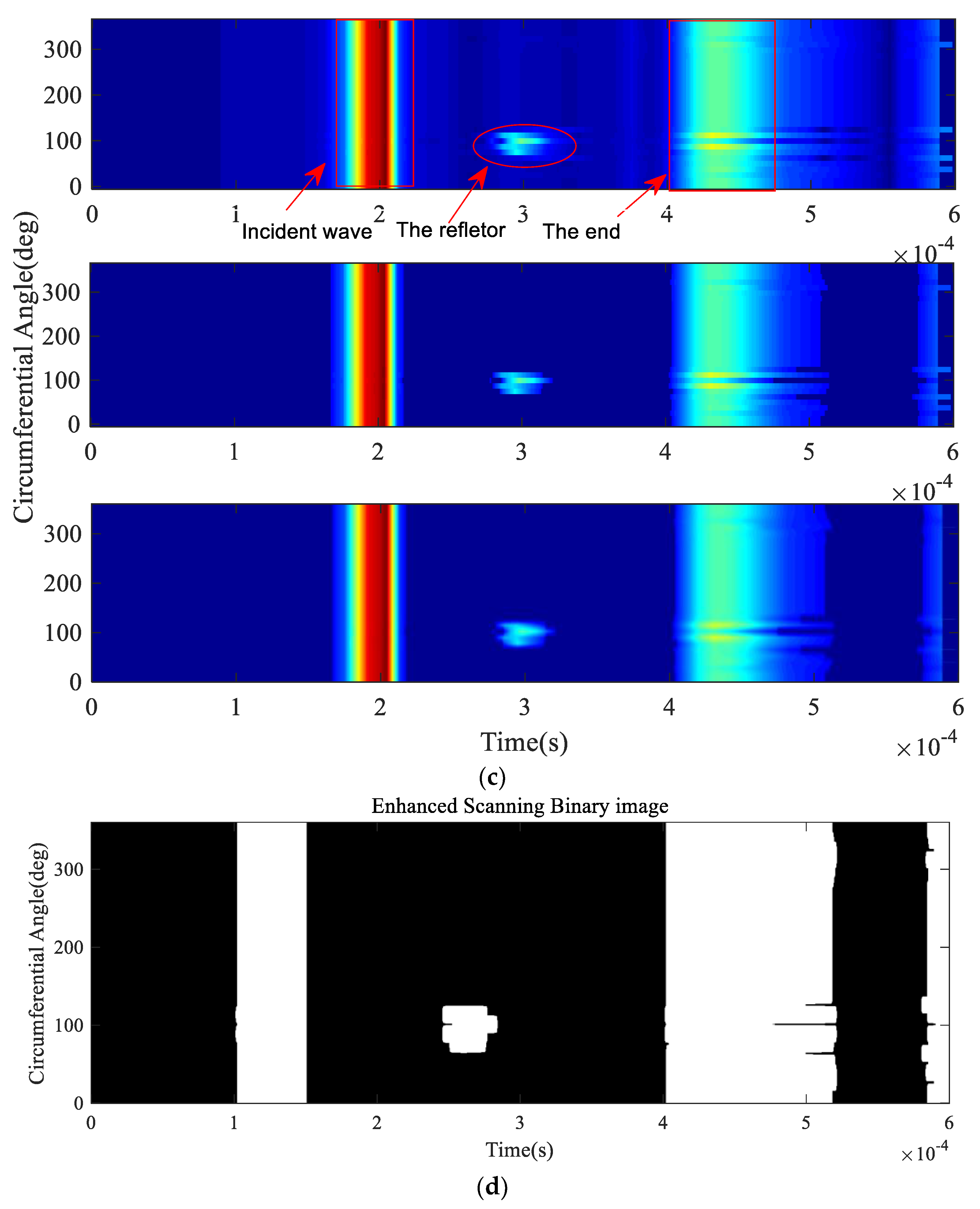
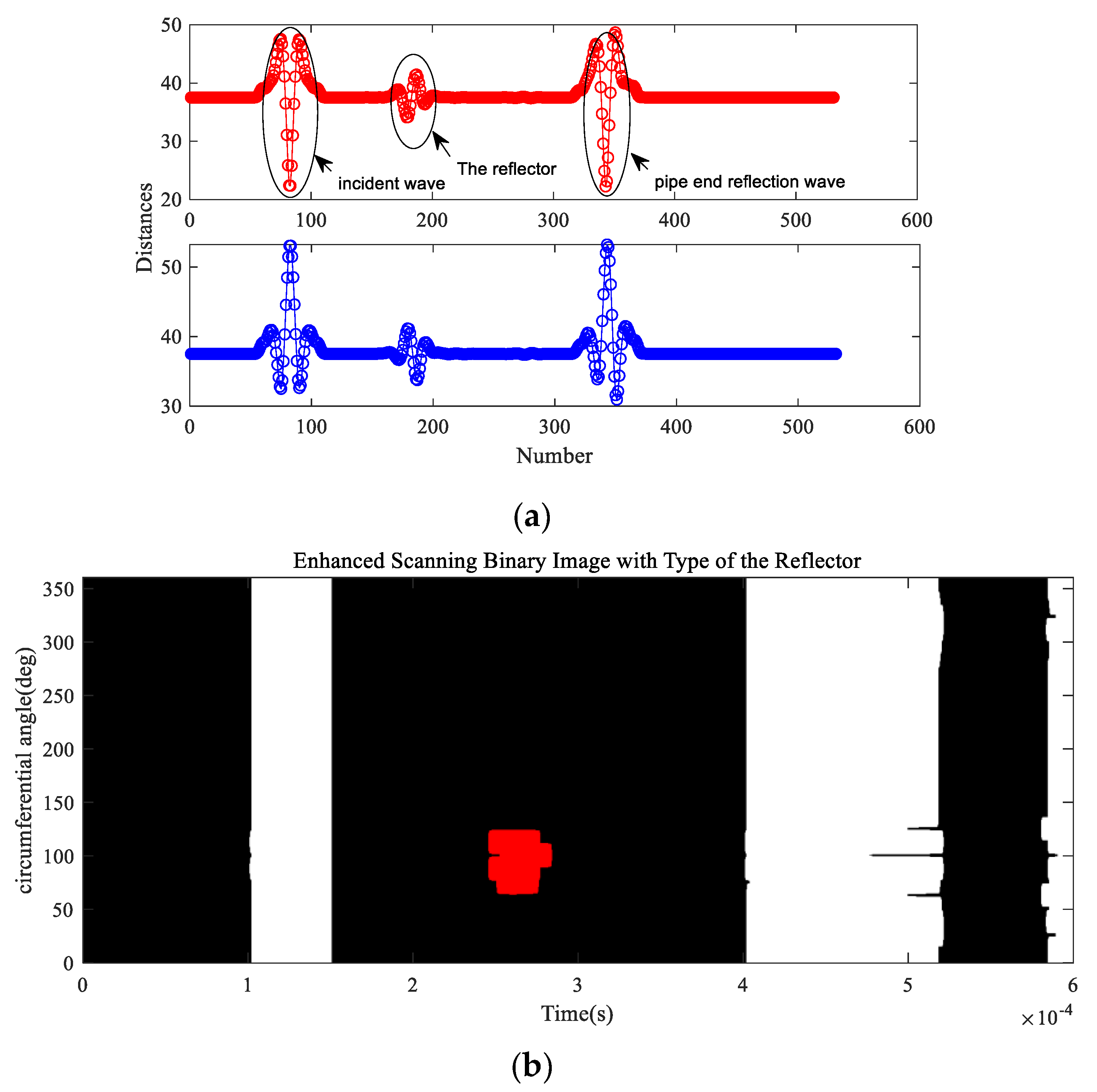
5.3. Simulation Investigation and Verification

The finite element (FE) is widely used to investigate the interaction between guided waves propagating along a structure and features within the structure [22,23,24,25,26,27]. In this section, in order to test the functionality and reliability of the proposed method, numerical simulations in sample pipes were conducted. The three-dimensional solid and finite element model of the sample pipes were constructed in a commercial FE software package [28].

5.3.1. Finite Element Model

As displayed by the three-dimensional schematic diagrams in Figure 10a,b, a sample pipe with an inner radius of r, an outer radius of J and a length of B is used. Circumferential grid nodes on one end of the pipe are chosen as the excitation nodes. Receiving nodes of guided-wave signals are E away from the excitation nodes. The reflector, whose front-edge is located F away from the excitation nodes, is characterized by the parameters of the axial length Z, the slope angle α, the radial depth Q and the circumferential extent β, respectively. Three test cases with different types of models depicted in Figure 10b were investigated. The geometrical and physical parameters of the sample pipes are listed in

Table 3. Geometrical and physical parameters of the sample pipes.

Category	Outer Radius (J)/mm	Inner Radius (r)/mm	Axial Length (Z)/mm	Circumferential Extent β/deg	Slope Angle α/deg	Depth (Q)/mm	Length (B)/mm	Length (F)/mm	Density Kg/m3	Distance (E)/mm	Poisson’s Ratio	Young’s Modulus/GPa	Reflector’s Type
Case 1	204	200	2	5	90	2	650	390	7800	230	0.28	210	Defect feature (Model 1)
Case 2	204	200	2	5	120	2	650	390	7800	230	0.28	210	Defect feature (Model 2)
Case 3	204	200	4	10	90	4	650	390	7800	230	0.28	210	Geometric feature (Model 3)
			2	8	90			318					Defect feature (Model 1)

. The physical parameters in all models include the Poisson’s ratio, Young’s modulus and density, which are set with the values for a steel pipe [6]. Model 1 and Model 2 represent reflectors with different structures, and their slope angles are different (typical values: 90° and 120°) in Cases 1 and 2. Considering that Case 3 contains multiple reflectors, to show the results clearly, the values of geometrical parameters in Case 3 are larger than those in Cases 1 and 2. The types of the reflectors in Model 1 and Model 2 are defect features, while Model 3 contains a geometric feature. The predicted results using the proposed method were presented and discussed below.

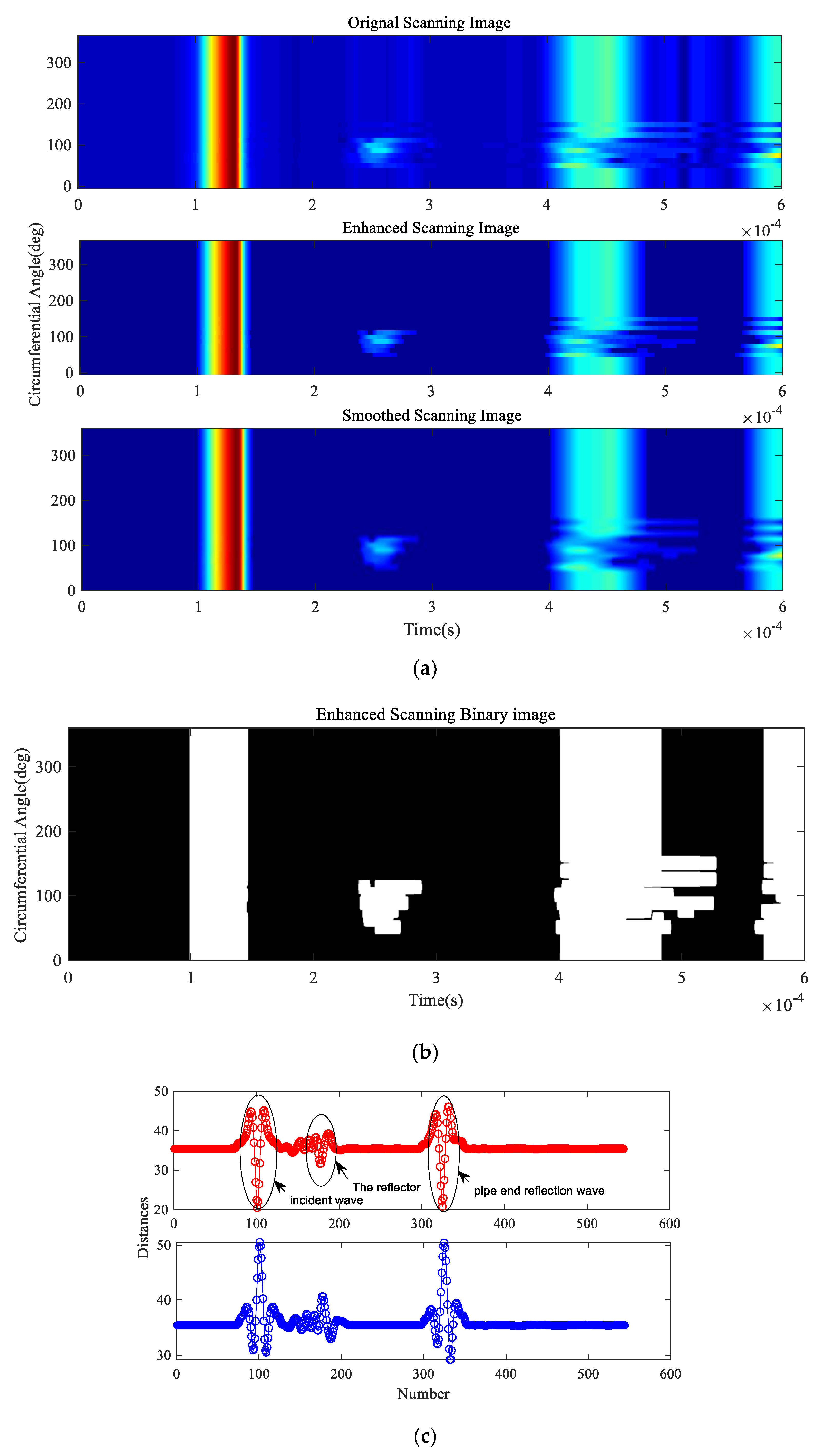
5.3.2. Investigation for Case 1

The numerical model of the test Case 1 with parameters shown in Table 3 was established in ABAQUS/Explicit, as illustrated in Figure 10b. This reflector was set on the outer surface of the pipe. The C3D8R type elements with mesh size l = 1 mm were used in the model to ensure convergence and solution accuracy. Steps (1) to (3) were performed first. As illustrated in Figure 2, the size of the transducer elements is approximately 48°, and the step is η = 12°, the circumferential displacements (uθ) were recorded and 30 sets of data were obtained after scanning along the pipe for 360°. The received signals formed a 2D data matrix H_i*j. The upper envelopes of H_i*j shown in Figure 11a were obtained by applying the Hilbert transform. Subsequently, the 3D representation of the scan results was illustrated in Figure 11b, and was constructed with the upper envelopes. In order to obtain the axial and circumferential positions of the reflector, the original scanned image was processed in order to improve the detection accuracy by applying a median filter, bilinear interpolation algorithm and binary processing; the enhanced 2D scanned image, smoothed 2D scanned image and enhanced 2D scanned binary image obtained are illustrated in Figure 11c,d respectively. The images were displayed as an unwrapped pipe, with the top and bottom of the images being at the same circumferential location, the vertical axis as the circumferential location, and the horizontal axis as the axial position. The axial and circumferential positions of the reflector are shown clearly in the images.

The end of the pipe and the incident signals are continuous from the bottom to the top in the scanned images, while the reflector is discontinuous and is located within a small circumferential range. To identify the reflector, steps (4) to (10) were further performed. Based on the wave structural characteristics of the torsional guided wave mode [29], the incident signal S_i(n) of the T(0,1) mode was generated by uniformly applying the excitation displacement of the Gabor pulse with parameters (σ, μ, θ_in, f_c) = (3 × 10⁻⁵ s, 1.5 × 10⁻⁵ s, π/2rad, 64 kHz) depicted in Equation (10) on the excitation nodes. The centre frequency f_c = 64 kHz is below the cut-off frequency of the T(0,2) mode shown in Figure 12. Therefore, the mode conversion was not considered in this study. The reflected signals S_r(n) were obtained through the receiving nodes.

The observation time is T = 6 × 10⁻⁴ s. The dimensions of S_i(n) and S_r(n) are Γ_I = 43 and Γ_r = 574 respectively. The analysis step γ is equal to 1, so the total number M = 531. Through steps (6) and (7), the standard Euclidian distance curves Ψ₁ and Ψ₂ were calculated in MATLAB and shown in Figure 13a. The minimum values of the distance curves were D₁ = 33.75 and D₂ = 34.11, respectively. D₁ < D₂, therefore the front-edge of the reflector was a step down, indicating that the reflector was a defect feature. The value of the RICR was equal to 1.43 (RICR > 1.05), thus the judgement is reliable. Finally, the enhanced 2D scanned binary image was updated and as shown in Figure 13b, the reflector was marked in red. The final Figure 13b presented the location information and character of the concerned reflector in an intuitive way.

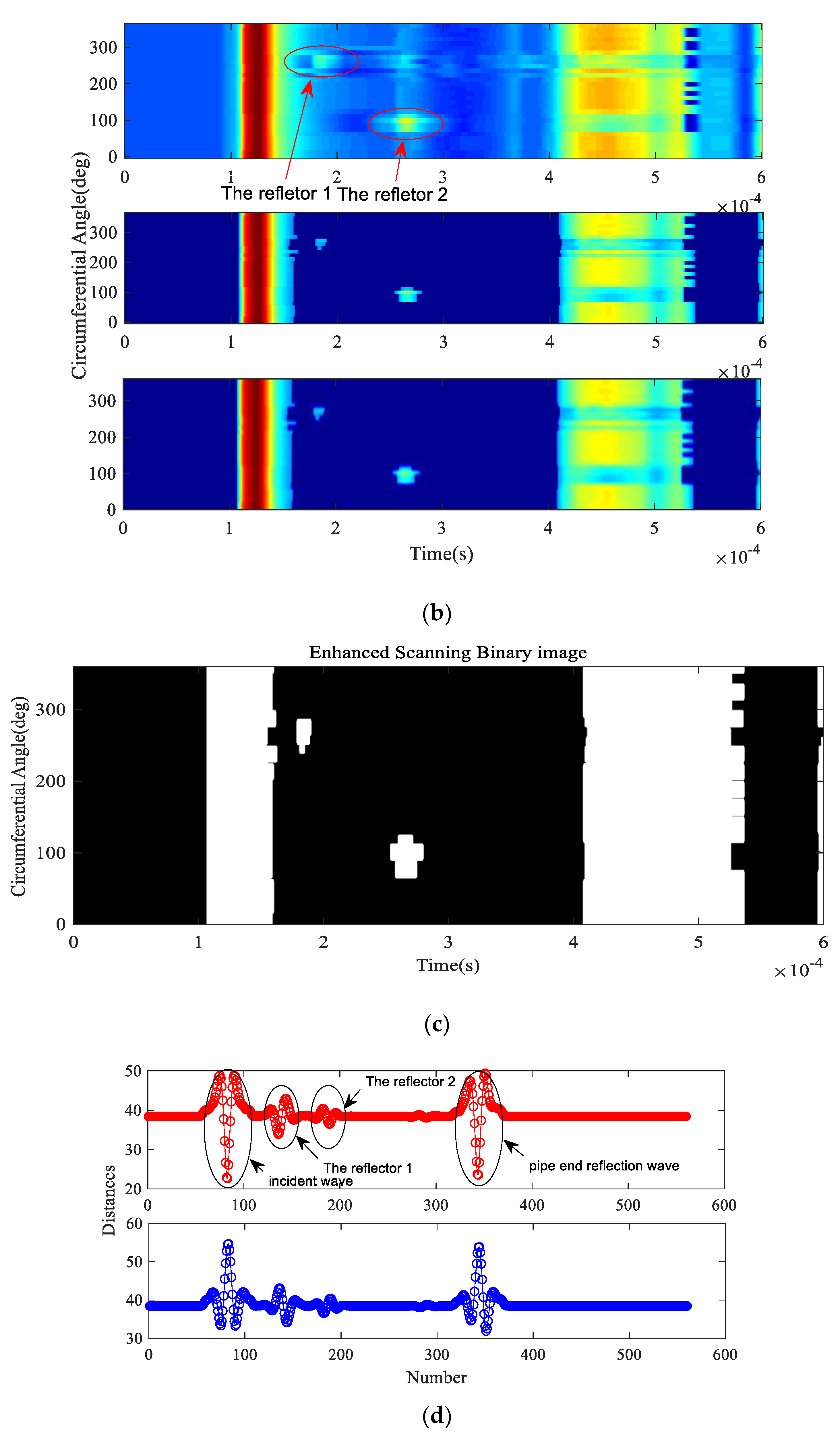
5.3.3. Investigation for Case 2

The geometrical and physical parameters of the steel pipe used in case 2 are shown in Table 3. Similarly, the 3D finite element model was constructed in ABAQUS/Explicit and steps (1) to (3) were performed first. After the circumferential scanning simulations, 30 sets of data were obtained in total, then the original scanned image, the enhanced 2D scanned image, smoothed 2D scanned image and enhanced 2D scanned binary image shown in Figure 14a,b were constructed with the simulated signals. The circumferential and axial positions of the reflector were displayed in the images clearly. In order to determine the type of the reflector, steps (4) to (10) were carried out. The displacement loads of the Gabor pulse excitation signal S_i(n) with parameters (σ, μ, θ_in, f_c) = (3e − 5s, 1.5e − 5s, π/2rad, 64 kHz) were uniformly applied in the tangential direction of the excitation nodes to generate the T(0,1), S_r(n) were obtained through the receiving nodes.

Through steps (6) and (7), Ψ₁ and Ψ₂ were calculated in MATLAB and shown in Figure 14c. The minimum values were D₁ = min{$D(S_i,S_{ri})$} = 31.65 and D₂ = min{$D(\overline{\overline{S_i}},S_{ri})$} = 32.97, respectively. D₁ < D₂, therefore the front-edge of the reflector was a step down, indicating the reflector to be a defect feature. The values of the RICR was equal to 3.75 (RICR > 1.05), thus the judgement was reliable. Finally, the result was updated to the final 2D image, as shown in Figure 14d.

5.3.4. Investigation for Case 3

Case 3 investigated multiple reflectors in a pipe. The parameters of the steel pipe used in Case 3 are shown in Table 3, and the 3D finite element model constructed and illustrated in Figure 15a is the combination of Model 1 and Model 3, as it contains two types of reflectors: a defect feature (reflector 1) and a geometric feature (reflector 2). The size of the transducer elements is about 60°, and the step is η = 12°. Steps (1) to (3) were performed first. After simulations, 30 sets of data were obtained, then the original scanned image, the enhanced 2D scanned image, smoothed 2D scanned image and enhanced 2D scanned binary image shown in Figure 15b,c were constructed. Compared with Figure 11c or Figure 14a, the reflection waves were strengthened when the size of the transducer elements was increased. To determine the type of the reflectors, steps (4) to (10) were carried out. Through loading the excitation displacement on the excitation nodes, S_r(n) were obtained by the receiving nodes.

Through steps (6) and (7), Ψ₁ and Ψ₂ were calculated in MATLAB and shown in Figure 15d. For reflector 1, D₁ = min{$D(S_i,S_{ri})$} = 33.95 and D₂ = min{$D(\overline{\overline{S_i}},S_{ri})$} = 34.22, D₁ < D₂, thus the front-edge of the reflector was a step down, indicating the reflector was a defect feature. The RICR was equal to 1.31 (RICR > 1.05), thus the judgement is reliable. For reflector 2: D₁ = 36.6 and D₂ = 36.5, D₁ > D₂, thus the front-edge of the reflector was a step up, indicating the reflector was a geometric feature. The value of the RICR was equal to 1.10 (RICR > 1.05), thus the judgement is reliable. Lastly, the enhanced 2D scanned binary image was updated with the results, as shown in Figure 15e.

6. Conclusions

In this paper, a novel method for locating and identifying pipeline reflectors is proposed based on guided-wave circumferential scanning and phase characteristics. The method is a combination of two different techniques. The first technique determines the circumferential and axial positions of the reflectors by circumferential scanning, leading to an enhanced 2D scanned binary image constructed from a series of image-processing methods used to improve the resolution and detection accuracy. The second technique utilizes the one-to-one phase characteristics between the incident wave and reflection waves to identify the change and type of reflector. Then, the predictions are updated to the enhanced 2D scanned binary images and marked with different colours. An identification index named the reliable index for the character of the reflector (RICR) was proposed to evaluate the reliability of the predicted results. FE software ABAQUS/Explicit was used to build 3D solid and finite element models of the sample pipes. Numerical signals with different SNRs and FE simulation signals with different models were successfully performed to validate the proposed method.

The proposed method and conclusions will offer guidance for further applications, and the findings presented in this paper can serve as a foundation. For future studies on this topic, other factors such as reflectors of different materials and geometric parameters as well as multi-modes of the guide wave will be investigated. Although numerical simulations have validated the proposed method, experimental validation will be conducted in future work.

References

1. Rao, J.; Ratassepp, M.; Lisevych, D.; Hamzah Caffoor, M.; Fan, Z. On-line corrosion monitoring of plate structures based on guided wave tomography using piezoelectric sensors. Sensors 2017, 17, 2882. [Google Scholar] [CrossRef] [PubMed] [Green Version]
2. Yu, X.; Fan, Z.; Puliyakote, S.; Castaings, M. Remote monitoring of bond line defects between a composite panel and a stiffener using distributed piezoelectric sensors. Smart Mater. Struct. 2018, 27, 035014. [Google Scholar] [CrossRef]
3. Lowe, M.J.S.; Alleyne, D.N.; Cawley, P. Defect detection in pipes using guided waves. Ultrasonics 1998, 36, 147–154. [Google Scholar] [CrossRef]
4. Alleyen, D.N. Long range propagation of lamb wave in chemical plant pipe-work. Mater. Eval. 1997, 55, 504–508. [Google Scholar]
5. Alleyne, D.N.; Pavlakovic, B.; Lowe, M.J.S.; Cawley, P. The use of guided waves for rapid screening of chemical plant pipework. J. Korean Soc. Nondestruct. Test. 2002, 22, 589–598. [Google Scholar]
6. Zhang, X.; Tang, Z.; Lv, F.; Yang, K. Scattering of torsional flexural guided waves from circular holes and crack-like defects in hollow cylinders. Ndt E Int. 2017, 89, 56–66. [Google Scholar] [CrossRef]
7. Alleyne, D.N.; Cawley, P. The effect of discontinuities on the long-range propagation of Lamb waves in pipes. Proc. Inst. Mech. Eng. Part E J. Process Mech. Eng. 1996, 210, 217–226. [Google Scholar] [CrossRef]
8. Galvagni, A.; Cawley, P. The reflection of guided waves from simple supports in pipes. J. Acoust. Soc. Am. 2011, 129, 1869–1880. [Google Scholar] [CrossRef]
9. Cawley, P.; Lowe, M.J.S.; Simonetti, F.; Chevalier, C.; Roosenbrand, A.G. The variation of the reflection coefficient of extensional guided waves in pipes from defects as a function of defect depth, axial extent, circumferential extent and frequency. Proc. Inst. Mech. Eng. Part C J. Mech. Eng. Sci. 2002, 216, 1131–1143. [Google Scholar] [CrossRef]
10. Alleyne, D.N.; Lowe, M.J.S.; Cawley, P. The reflection of guided waves from circumferential notches in pipes. J. Appl. Mech. 1998, 65, 635–641. [Google Scholar] [CrossRef]
11. Løvstad, A.; Cawley, P. The reflection of the fundamental torsional guided wave from multiple circular holes in pipes. Ndt E Int. 2011, 44, 553–562. [Google Scholar] [CrossRef]
12. Demma, A.; Cawley, P.; Lowe, M.; Roosenbrand, A.G.; Pavlakovic, B. The reflection of guided waves from notches in pipes: A guide for interpreting corrosion measurements. Ndt E Int. 2004, 37, 167–180. [Google Scholar] [CrossRef]
13. Sargent, J.P. Corrosion detection in welds and heat-affected zones using ultrasonic Lamb waves. Insight Nondestruct. Test. Cond. Monit. 2006, 48, 160–167. [Google Scholar] [CrossRef] [Green Version]
14. Muñoz, C.Q.G.; Marquez, F.P.G.; Lev, B.; Arcos, A. New pipe notch detection and location method for short distances employing ultrasonic guided waves. Acta Acust. United Acust. 2017, 103, 772–781. [Google Scholar] [CrossRef] [Green Version]
15. Mu, J.; Zhang, L.; Rose, J.L. Defect circumferential sizing by using long range ultrasonic guided wave focusing techniques in pipe. Nondestruct. Test. Eval. 2007, 22, 239–253. [Google Scholar] [CrossRef]
16. Li, J. On circumferential disposition of pipe defects by long-range ultrasonic guided waves. J. Press. Vessel Technol. 2005, 127, 530–537. [Google Scholar] [CrossRef]
17. Wu, J.; Tang, Z.; Yang, K.; Wu, S.; Lv, F. Ultrasonic Guided Wave-Based Circumferential Scanning of Plates Using a Synthetic Aperture Focusing Technique. Appl. Sci. 2018, 8, 1315. [Google Scholar] [CrossRef] [Green Version]
18. Zhang, X.; Tang, Z.; Lü, F.; Pan, X. Excitation of dominant flexural guided waves in elastic hollow cylinders using time delay circular array transducers. Wave Motion 2016, 62, 41–54. [Google Scholar] [CrossRef]
19. Alleyne, D.N.; Pavlakovic, B.; Lowe, M.J.S.; Cawley, P. Rapid, Long Range Inspection of Chemical Plant Pipework Using Guided Waves. Key Eng. Mater. 2004, 270–273, 434–441. [Google Scholar] [CrossRef]
20. Auld, B.A.; Green, R.E. Acoustic Fields and Waves in Solids: Two Volumes. Phys. Today 1974, 27, 63. [Google Scholar] [CrossRef]
21. Gabor, D. Theory of communication. J. Inst. Electr. Eng. Part III Radio Commun. Eng. 1946, 93, 429–457. [Google Scholar] [CrossRef]
22. Zhu, W. An FEM simulation for guided elastic wave generation and reflection in hollow cylinders with corrosion defects. J. Press. Vessel. Technol. 2001, 124, 108–117. [Google Scholar] [CrossRef]
23. Moser, F.; Jacobs, L.J.; Qu, J. Modeling elastic wave propagation in waveguides with the finite element method. Ndt E Int. 1999, 32, 225–234. [Google Scholar] [CrossRef]
24. Hayashi, T.; Kawashima, K.; Sun, Z.; Rose, J.L. Analysis of flexural mode focusing by a semianalytical finite element method. J. Acoust. Soc. Am. 2003, 113, 1241–1248. [Google Scholar] [CrossRef] [PubMed] [Green Version]
25. Gravenkamp, H.; Birk, C.; Song, C. Simulation of elastic guided waves interacting with defects in arbitrarily long structures using the scaled boundary finite element method. J. Comput. Phys. 2015, 295, 438–455. [Google Scholar] [CrossRef]
26. Zuo, P.; Yu, X.; Fan, Z. Numerical modeling of embedded solid waveguides using SAFE-PML approach using a commercially available finite element package. Ndt E Int. 2017, 90, 11–23. [Google Scholar] [CrossRef]
27. Zuo, P.; Zhou, Y.; Fan, Z. Numerical studies of nonlinear ultrasonic guided waves in uniform waveguides with arbitrary cross sections. AIP Adv. 2016, 6, 075207. [Google Scholar] [CrossRef] [Green Version]
28. Abaqus Analysis User’s Guide. Version 6.16. Available online: https://www.3ds.com/products-services/simulia/products/abaqus/ (accessed on 12 November 2019).
29. Rose, J.L. Ultrasonic Guided Waves in Solid Media; Cambridge University Press: Cambridge, UK, 2014. [Google Scholar]
Figure 1. Schematic of guided wave propagating in the pipe inspection.
Applsci 10 01799 g001
Figure 2. Schematic showing the pipe and its unrolled image by the guided-wave circumferential scanning technique: (a) numerical model; (b) circumferential scanning image.
Applsci 10 01799 g002
Figure 3. Numerical simulation results of guided-wave A-scan and circumferential scanning in pipes by finite element software: (a) an undamaged pipe; (b) a pipe with a girth weld; (c) A-scan signal of the pipe; (d) A-scan signal of the girth weld; (e) circumferential scanned image of the pipe; (f) circumferential scanned image of the girth weld.
Applsci 10 01799 g003
Figure 4. Guided wave propagation in a pipe and reflection coefficient (RC) in the complex plane: (a) guided wave propagation in a pipe with a reflector; (b) RC in the complex plane.
Applsci 10 01799 g004
Figure 5. A reflector can be decomposed into a step down and a step up.
Applsci 10 01799 g005
Figure 6. Wave propagation paths corresponding to the individual signals in a pipe with a reflector.
Applsci 10 01799 g006
Figure 7. Reflection wave from the front- and back-edge of a reflector and their overlapping wave: (a) reflection wave from a reflector; (b) overlapping wave.
Applsci 10 01799 g007
Figure 8. Numerical signals with different signal-to noise ratios (SNRs) and comparisons of the results by the proposed method and correlation coefficient method; (a) x ^ 1 ( t ) with SNR = 1 dB; (b) Distance curves Ψ1 (Up) and Ψ2 (Down) of x ^ 1 ( t ) ; (c) x ^ 2 ( t ) with SNR = 0.1 dB; (d) Distance curves Ψ1 (Up) and Ψ2 (Down) of x ^ 2 ( t ) ; (e) Pearson’s correlation coefficient method (PCCM) curves Ψ1 (Up) and Ψ2 (Down) of x ^ 1 ( t ) ; (f) PCCM curves Ψ1 (Up) and Ψ2 (Down) of x ^ 2 ( t ) .
Applsci 10 01799 g008
Figure 9. Numerical signals with different SNRs and comparisons of the results by the proposed method and correlation coefficient method; (a) x ^ 1 ( t ) with SNR = 1 dB; (b) Distance curves Ψ1 (Up) and Ψ2 (Down) of x ^ 1 ( t ) ; (c) x ^ 2 ( t ) with SNR = 0.1 dB; (d) Distance curves Ψ1 (Up) and Ψ2 (Down) of x ^ 2 ( t ) ; (e) PCCM curves Ψ1 (Up) and Ψ2 (Down) of x ^ 1 ( t ) ; (f) PCCM curves Ψ1 (Up) and Ψ2 (Down) of x ^ 2 ( t ) .
Applsci 10 01799 g009aApplsci 10 01799 g009b
Figure 10. Schematic illustration of the finite element models in the sample pipe: (a) three-dimensional schematic diagram; (b) schematic of a sample pipe with different types of models.
Applsci 10 01799 g010
Figure 11. Analysis results based on the proposed method: (a) the upper envelopes of the guided-wave simulation signals: (b) 3D representation of the reflector; (c) original 2D scanned image (Up), enhanced 2D scanned image (Middle) and smoothed 2D scanned image (Down); (d) enhanced 2D scanned binary image.
Applsci 10 01799 g011aApplsci 10 01799 g011b
Figure 12. Dispersion curves of pipes illustrated in Table 1: (a) phase velocity curves; (b) group velocity curves.
Applsci 10 01799 g012
Figure 13. Analysis results based on the proposed method; (a) distance curves Ψ1 (Up) and Ψ2 (Down); (b) updated judgment results to the enhanced 2D scanned binary image with different colours.
Applsci 10 01799 g013
Figure 14. Analysis results based on the proposed method: (a) original 2D scanned image (Up), enhanced 2D scanned image (Middle) and smoothed 2D scanned image (Down); (b) enhanced 2D scanned binary image; (c) distance curves Ψ1 (Up) and Ψ2 (Down); (d) updated judgment results to the enhanced 2D scanned binary image with different colours.
Applsci 10 01799 g014aApplsci 10 01799 g014b
Figure 15. Analysis results based on the proposed method: (a) a sample pipe with two reflectors; (b) original 2D scanned image (Up), enhanced 2D scanned image (Middle) and smoothed 2D scanned image (Down); (c) enhanced 2D scanned binary image; (d) distance curves Ψ1 (Up) and Ψ2 (Down); (e) updated judgment results to the enhanced 2D scanned binary image with different colours.
Applsci 10 01799 g015aApplsci 10 01799 g015bApplsci 10 01799 g015c