Modeling the Accuracy of Estimating a Neighbor’s Evolving Position in VANET

Abstract

Accurate estimation of a neighbor’s evolving position is essential to enhancing safety in intelligent transport systems. A vehicle can estimate a neighbor’s evolving position via periodic beaconing wherein each vehicle periodically broadcasts a beacon including its own kinematic data (e.g., position, speed, and acceleration). Many researchers have proposed analytic models to describe periodic beaconing in vehicular ad-hoc networks (VANETs). However, those models have focused only on network performance, e.g., packet delivery ratio (PDR), or a delay, which fail to evaluate the accuracy of estimating a neighbor’s evolving position. In this paper, we present a new analytic model capable of providing an estimation error of a neighbor’s evolving position in VANET to assess the accuracy of the estimation. This model relies on a vehicle system using periodic beaconing and a constant speed and position estimator (CSPE) to estimate a neighbor’s evolving position. To derive an estimation error, we first calculate the estimation error using a simple equation, which is associated with a probability of successful reception. Then, we derive the probability of successful reception that is applied onto the error model. To our knowledge, this is the first paper to establish a mathematical model to assess the accuracy of estimating a neighbor’s evolving position. To validate the proposed model, we compared the numerical results of the model with those of the NS-2 simulation. We observed that numerical results of the proposed model were located within the 95% confidential intervals of simulations results.

1. Introduction

Vehicular ad-hoc networks (VANETs) are the driving force for realizing intelligent transport systems such as vehicular safety systems and autonomous driving systems. In these systems, accurate positioning of surrounding vehicles (i.e., neighbors) is essential to securing safety of a driver. As the technology for connected vehicles has become more widespread, periodic beaconing has become fundamental for the accurate positioning. Specifically, each vehicle periodically broadcasts a beacon message including its kinematic data (e.g., position, velocity, and acceleration). Upon receiving this message, vehicles can estimate the evolving position of the sender of the message.

Several mathematical models were proposed when periodic beaconing was adopted in VANET [1,2,3,4,5,6,7,8,9]. In [1,2], the authors proposed packet delivery ratio (PDR) and delay models in which multi-channel operation was considered. The authors in [3] focused on the possible effects of a hidden terminal problem in establishing a PDR model. In [4], the authors established an analytic model that incorporated the hidden terminal problem and general service time distribution. In the PDR model proposed in [5], a statistical channel model was considered. In [6], the authors developed a model for delay distribution on periodic beaconing. In [7,8], an analytic model focused on 802.11p EDCA performance was established based on Markov chain models. In [9], the authors developed an analytic model for the delay distribution of a safety message’s dissemination using a white TV spectrum.

The limitation of the previous models involves focusing only on network performances (e.g., PDR and delay) that fail to evaluate the accuracy of estimating a neighbor’s evolving position in intelligent transport systems. Specifically, the accuracy can be quantified with an estimation error of a neighbor’s evolving position, but the network performances cannot be directly translated into the estimation error. For example, as shown in Figure 1, the estimation error of a neighbor’s evolving position could be different even with the same PDR. Even if PDR in Figure 1a is the same as that in Figure 1b (0.5), the error in estimating the position of VEH 2 by VEH 1 is 0.75 m in Figure 1a, whereas the estimation error is 0.5 m in Figure 1b. In [10], the authors proposed a model for tracking uncertainty when periodic beaconing was adopted. However, the tracking uncertainty is an upper bound of a tracking error rather than a specific value for the tracking error. In [11], the authors proposed a congestion control algorithm depending on estimating tracking error and channel load. However, the authors did not provide a mathematical model for tracking error but the algorithm for getting the approximate tracking error in real time.

Figure 1. Estimation error of a neighbor’s position can be different even with the same packet delivery ratio (PDR).

To address this limitation of previous models, in this paper, we propose a new analytic model for an estimation error of a neighbor’s evolving position in VANET (The estimated position is the absolute position of the neighbor). To derive the estimation error, we consider that a vehicle estimates a neighbor’s evolving position using a constant speed and position estimator (CSPE) and kinematic data of the beacon received from the neighbor. In the CSPE, the current position of a neighbor is estimated using a position and a velocity included in a received beacon. To establish a mathematical model, we first establish a model for the estimation error using a simple equation, which is associated with a probability of successful reception. Then, we obtain the probability of successful reception that will be used in the error model. To the best of our knowledge, this is the first attempt to establish an analytic model for evaluating the accuracy of estimating a neighbor’s evolving position in VANET. To validate the proposed model, we compare numerical results of our model with those of the NS-2 simulation [12]. We observe that numerical results of the proposed model are located within the 95% confidential intervals of simulation results and confirm that our model is accurate (The numerical results of our model are calculated from Equation (5), which adopts the $p_s$ derived in Section 2.3). It is noted that we can use statistics on the estimation error obtained from the proposed model in designing an algorithm for optimal parameter configurations.

The contributions of this paper are as follows.

• We establish the first analytic model for expressing an estimation error of a neighbor’s evolving position to evaluate the accuracy of the estimation.
• We validate the proposed model by comparing the numerical results of the model with the NS-2 simulation results.

The remainder of this paper is organized as follows. In Section 2, we explain the mathematical model of estimation error of neighbor’s evolving position. In Section 3, we validate the proposed model by comparing the numerical results of our model with those of the NS-2 simulation. This paper concludes with Section 4.

2. Analytic Model for the Estimation Error of a Neighbor’s Evolving Position

In this section, we explain the system model that is used for establishing our mathematical model and then present the step-by-step mathematical derivation of an estimation error of a neighbor’s evolving position. For the mathematical derivation, we first calculate the estimation error using a simple equation, which is associated with a probability of successful reception. Then, we describe the probability of successful reception in more detail. We summarize the notation used for mathematical mode in Table 1.

Table 1. Notation for the mathematical model.

${\mathit{x}}_{\mathit{c}\mathit{u}\mathit{r}}$	Actual current position of a neighbor
$a\left(t\right)$	Acceleration at time t
$v\left(t\right)$	Velocity of a neighbor at time t
$\beta$	Vehicle density
R	Transmission range
$T_{BI}$	Beacon interval
$\lambda$	Packet arrival rate
$\rho$	Probability that a buffer is not empty
$\tau$	Transmission attempt probability
$P_{busy}$	Probability of busy channel
$E\left[S\right]$	Average service time
$C{W}_{min}$	Minimum contention window size
$E\left[slot\right]$	Average slot time
$T_{data}$	Transmission duration of a beacon
$\sigma$	Duration of an empty slot time

2.1. System Model

We make some assumptions for establishing an analytic model. First, it is assumed that vehicles are deployed along a one-dimensional line topology. This assumption is reasonable because the width of a lane is negligible compared to the length of a road, particularly in highway areas. Second, we assume that the arrival of a message follows the Poisson process, similarly to several previous models on periodic beaconing [3,5,13].

In our model, each vehicle estimates evolving positions of vehicles within transmission range. For ease of explanation, we call a vehicle within a transmission range a “neighbor” and a vehicle estimating an evolving position of a neighbor an “ego vehicle.” Similarly to [10,11], we adopt a constant speed position estimator (CSPE) to estimate an evolving position of a neighborSpecifically, an ego vehicle calculates an evolving position of its neighbor at every beacon interval (BI) using kinematic information in the beacon and CSPE. Figure 2 illustrates how an ego vehicle estimates an evolving position of its neighbor. When receiving a beacon from N-VEH, an ego vehicle exploits position information in the beacon (e.g., the first estimation attempt in Figure 2). Failing to receive such a beacon message from N-VEH, an ego vehicle relies on a linear equation for CSPE with those most recently received (e.g., the second and the third estimation attempts in Figure 2). In our model, an ego vehicle fails to receive beacons from its neighbors when packet collision happens. We describe vehicle mobility with two random processes: (1) the number of vehicles passing a tagged point in a road (previous work on traffic flow revealed that the number of vehicle arrivals could be accurately modeled with the Poisson arrival process [14]) and (2) an acceleration from among those vehicles. For analytical tractability, we take a snapshot to gather statistics on periodic beaconing and kinematic data of vehicles at certain times, and then derive an estimation error of neighbors’ evolving positions at those moments. At each snapshot, the acceleration of a vehicle follows a random variable with the mean $a_m$. (In a practical scenario, we can obtain the average acceleration by averaging the acceleration information contained in the beacons received from neighbors). Here, we can use any random variable for modeling an acceleration. The benefit of this approach is that we can describe various mobility patterns by using a random variable corresponding to the mobility pattern.

Figure 2. The method for estimating a neighbor’s evolving position varies depending on whether an ego vehicle receives a beacon.

Using the mobility model with constant mean acceleration does not reduce the accuracy of a model because an acceleration rarely changes within a short interval in the real-world (i.e., piecewise constant). Specifically, the duration for gathering statistics of our model is short (e.g., order of a few seconds) and the abrupt changes in acceleration within this duration rarely occur in the real world. Thus, we can insist that the acceleration is constant for that short duration. To justify the mobility model with constant mean acceleration, we captured the mean acceleration over time using two mobility models (Krauss car-following model with and without lane-changing models) in SUMO. Then, we investigated the time-varying trend of the accelerations captured every 10 s. Figure 3 demonstrates that the mean acceleration is almost constant within 10 s window (black dotted box) except for some time points (red circle). However, as the proportion of those time points is very small, we can conclude that our mobility model with constant acceleration is valid.

Figure 3. Average acceleration according to time in 2 by 2 grid obtained by SUMO: (a) Krauss model without lane changing model and (b) Krauss model with lane changing model.

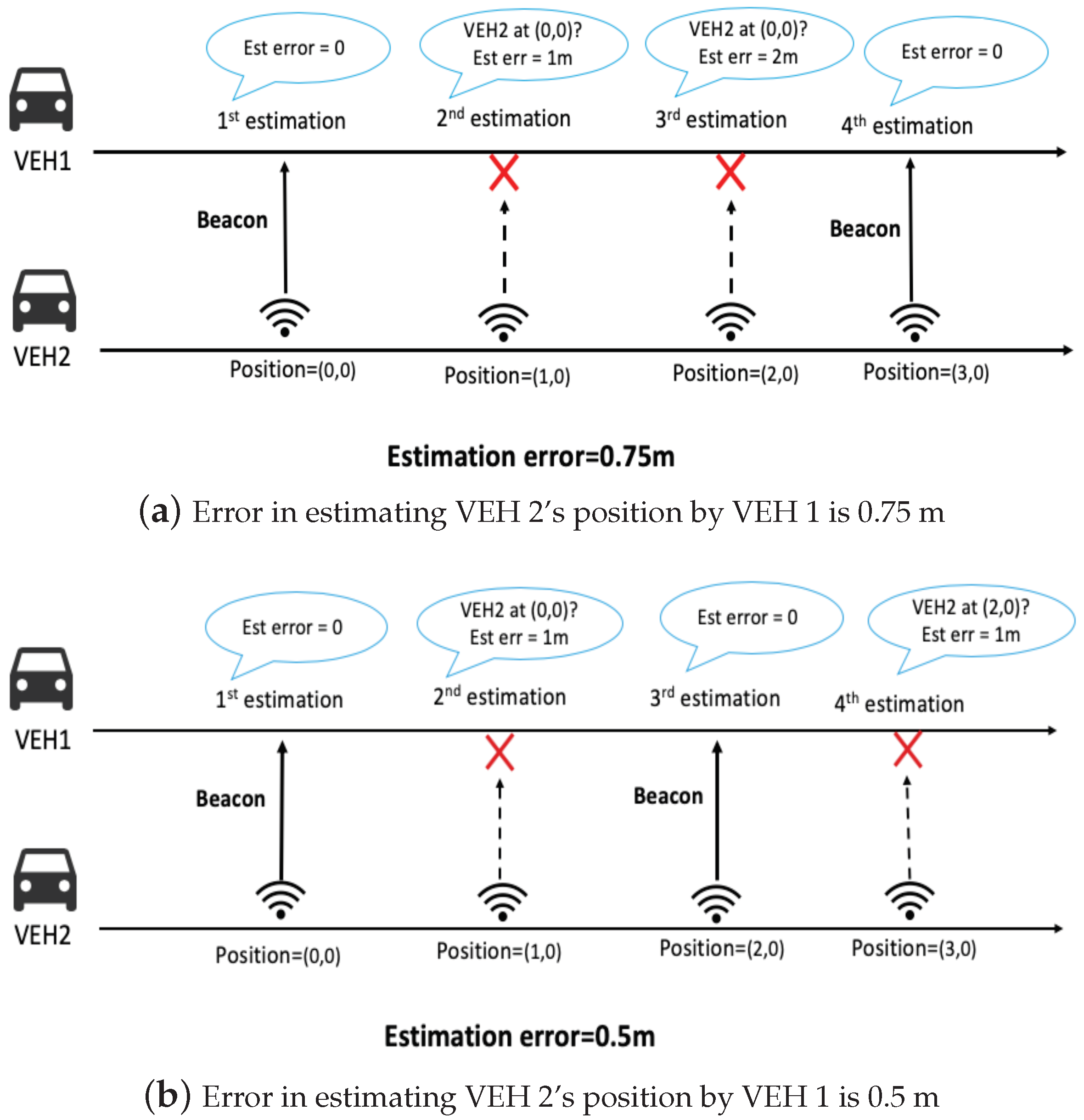
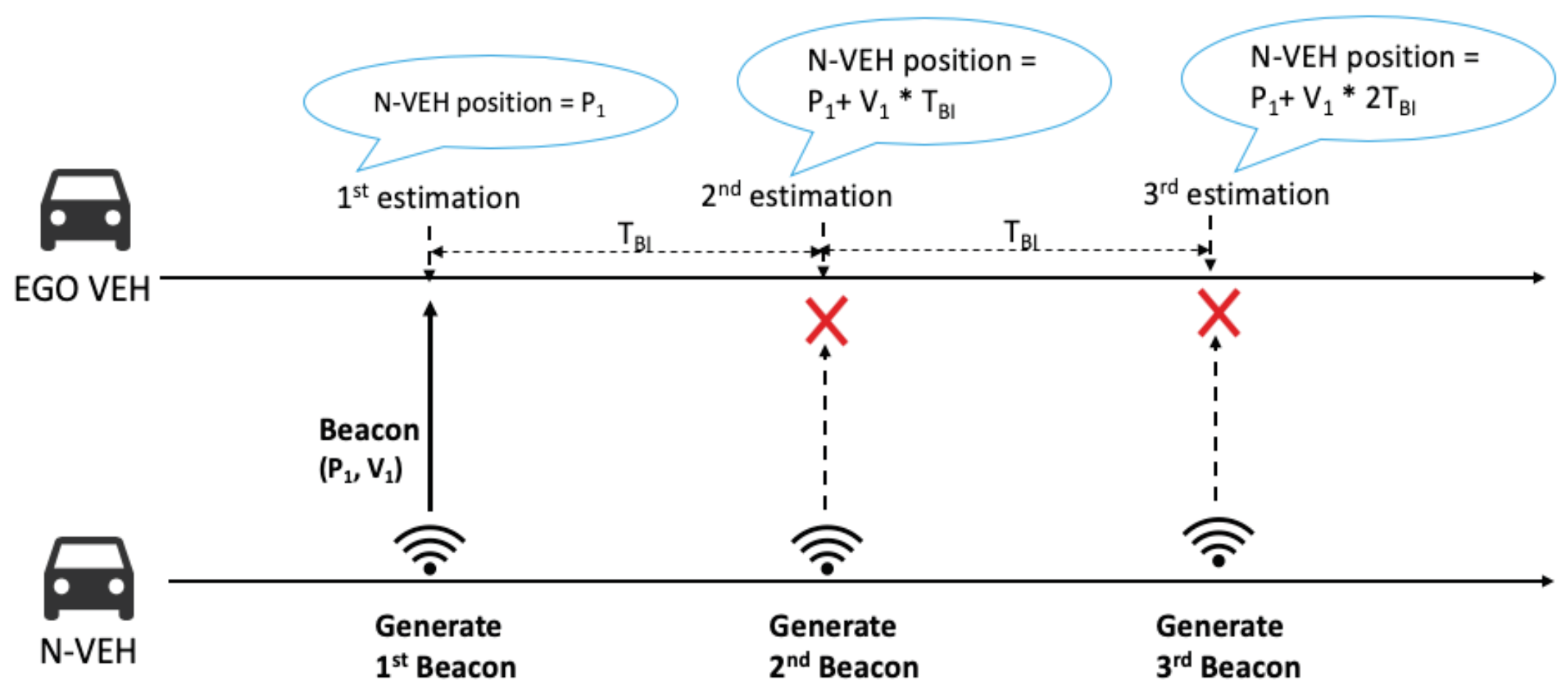
2.2. Estimation Error of a Neighbor’s Evolving Position

The procedure for deriving an estimation error of a neighbor’s evolving position consists of two steps. In the first step, we derive an estimation error according to two variables: (1) an acceleration of a neighbor (a) and (2) $n_f$. Here, $n_f$ represents the number of failures in receiving a beacon by an ego vehicle from the most recent reception of a beacon (e.g., $n_f=1$ at the second estimation and $n_f=2$ at the third estimation in Figure 2). In the second step, we average the estimation error obtained in step one over the two variables.

First, we derive the estimation error according to two variables, which can be obtained by

$$e_{n_f,a}^{est}=x_{cur}-{\tilde{x}}_{n_f,a}$$

(1)

where $x_{cur}$ is the current position of a neighbor and ${\tilde{x}}_{n_f,a}$ is an estimated position according to two variables, $n_f$ and a. $x_{cur}$ and ${\tilde{x}}_{n_f,a}$ can be described as

$$\begin{array}{cc}\hfill & x_{cur}=x_0+{\int }_0^{n_f{T}_{BI}}v(\tau )d\tau \hfill \\ \hfill & {\tilde{x}}_{n_f,a}=x_0+v\left(0\right)·n_f{T}_{BI}\hfill \end{array}$$

(2)

where $x_0$ is an actual position of a neighbor at the time when an ego vehicle receives a beacon from a neighbor. Here, we set the time of receiving a beacon by an ego vehicle to 0 for the ease of explanation. However, we can set this time to another value without reducing the accuracy of our model. $v(\tau )$ is the velocity of a neighbor at time $\tau$; $T_{BI}$ is a beacon interval. By applying Equation (2) to Equation (1), we can express $e_{n_f,a}^{est}$ as

$$\begin{array}{cc}\hfill e_{n_f,a}^{est}& ={\int }_0^{n_f{T}_{BI}}(v(\tau )-v\left(0\right))d\tau \hfill \\ \hfill & ={\int }_0^{n_f{T}_{BI}}({\int }_0^{\tau }a\left(u\right)du)d\tau \hfill \end{array}$$

(3)

where $a\left(u\right)$ is an acceleration at time u.

Second, we average $e_{n_f,a}^{est}$ over a and can obtain the estimation error according to $n_f$ ($e_{n_f}^{est}$) as follows.

$$\begin{array}{cc}\hfill e_{n_f}^{est}& =E_a\left[e_{n_f,a}^{est}\right]\hfill \\ \hfill & ={\int }_0^{n_f{T}_{BI}}({\int }_0^{\tau }{E}_a\left[a\left(u\right)\right]du)d\tau \hfill \\ \hfill & ={\int }_0^{n_f{T}_{BI}}(a_m\tau )d\tau \hfill \\ \hfill & =\frac{a_m}{2}·T_{BI}^2·n_f^2\hfill \end{array}$$

(4)

where $a_m$ is an average acceleration.

Finally, we average $e_{n_f}^{est}$ over $n_f$ to get an estimation error $e^{est}$, which can be expressed as

$$\begin{array}{cc}\hfill e^{est}& =E_{n_f}\left[e_{n_f}^{est}\right]\hfill \\ \hfill & =\sum _{n=0}^{n_f^{max}}\frac{a_m}{2}·T_{BI}^2·n^2·p_{n|n_f^{max}}\hfill \\ \hfill & =\sum _{n=0}^{n_f^{max}}\frac{a_m}{2}·T_{BI}^2·n^2·\frac{{(1-p_s)}^n·p_s}{1-{(1-p_s)}^{n_f^{max}+1}}\hfill \end{array}$$

(5)

where $n_f^{max}$ is the maximum number of $n_f$, and $p_{n|n_f^{max}}$ is a probability that $n_f$ is equal to n on the condition that $n_f\le n_f^{max}$. $n_f$ is equal to n when the following two events happen simultaneously. First, an ego vehicle must receive a beacon from the neighbor. Second, after the beacon reception, the ego vehicle must not have received a beacon n times from the neighbor. Thus, $p_{n|n_f^{max}}$ can be expressed as $\frac{{(1-p_s)}^n·p_s}{1-{(1-p_s)}^{n_f^{max}+1}}$ where $p_s$ is a probability of successful reception. We derive $p_s$ in the next subsection.

2.3. Derivation of the Probability of Successful Reception

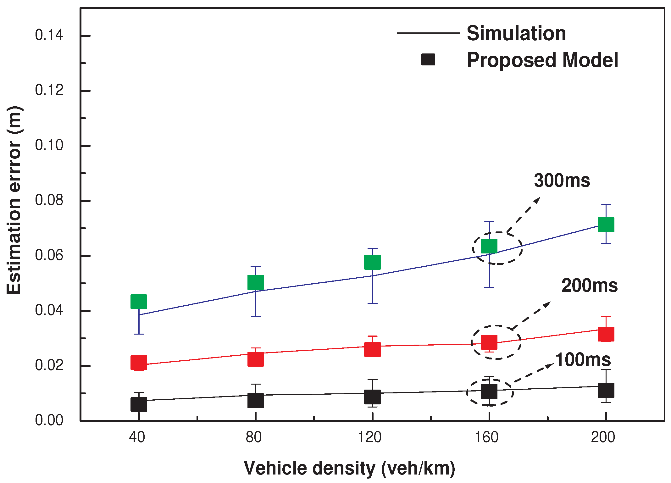
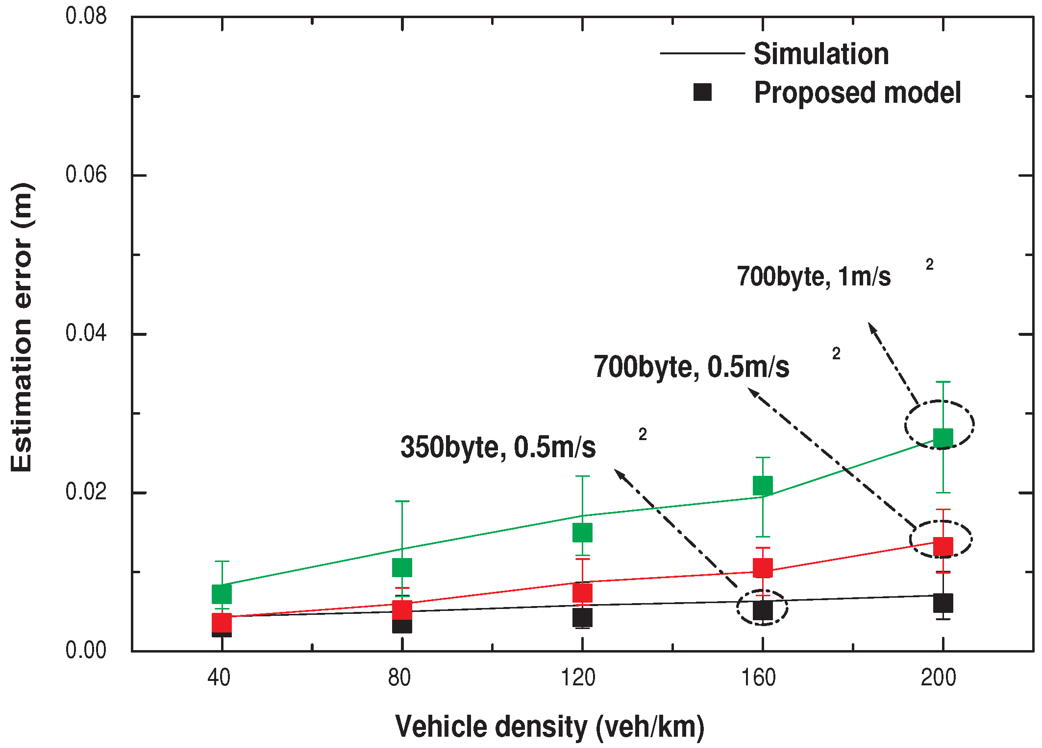
A vehicle successfully receives a beacon when two events occur simultaneously: (1) a direct collision does not occur and (2) a hidden collision does not happen. Thus, a probability of successful reception can be calculated by [5]

$$\begin{array}{cc}\hfill p_s& =P\left(X_D\right)·P\left(X_H\right)\hfill \end{array}$$

(6)

where $X_D$ is an event that a signal from a sender does not interfere with signals from any direct collisioners (DCs); $X_H$ is an event in which a signal from a sender does not interfere with signals from any hidden collisioners (HCs). Here, DC refers to a vehicle that could induce direct collisions at a receiver and HC refers to a hidden vehicle that might cause hidden collisions at a receiver.

The event $\overline{X_D}$ (the complement of an event $X_D$) happens when two events occur simultaneously: (1) a sender broadcasts a beacon and (2) at least one DC transmits a signal. First, a sender can broadcast its beacon only if it has a non-empty buffer ($\rho$) and the channel is idle ($1-P_{busy}$). Second, the complement of the second event is that no DC transmits a signal (${(1-\rho \tau )}^{N_D}$). Hence, $P\left(\overline{X_D}\right)=1-P\left(X_D\right)$ can be expressed by

$$\begin{array}{cc}\hfill & P\left(\overline{X_D}\right)\hfill \\ \hfill & =\rho (1-P_{busy})(1-{(1-\rho \tau )}^{N_D})\hfill \end{array}$$

(7)

where $\rho$ is the probability of a non-empty queue; $N_D$ is the number of DCs and can be expressed with $2\beta R$; $\beta$ is a vehicle density; R is a transmission range; $\tau$ is a transmission attempt probability and can be obtained by $\frac{2}{C{W}_{min}+1}$[15]; and $P_{busy}$ is the probability that a channel is busy. According to a queuing theory [16], $\rho$ can be expressed as $\lambda ·E\left[S\right]$ where $\lambda$ and $E\left[S\right]$ are an averaged message arrival rate and expected service time, respectively. $E\left[S\right]$ can be obtained by

$$\begin{array}{cc}\hfill & E\left[S\right]=T_{data}+(1-(1-\rho )(1-P_{busy}))·\overline{CW}·E\left[slot\right]\hfill \\ \hfill & \overline{CW}=\frac{C{W}_{min}+1}{2}\hfill \end{array}$$

(8)

where $C{W}_{min}$ is the minimum contention window size. $E\left[slot\right]$ is an average slot time and can be obtained by

$$E\left[slot\right]=\sigma ·(1-P_{busy})+T_{data}·P_{busy}$$

(9)

where $\sigma$ is the duration of an empty slot time and $T_{data}$ is the transmission duration of a beacon. $P_{busy}$ is obtained by

$$P_{busy}=1-{(1-\rho \tau )}^{N_D}$$

(10)

The event $X_H$ occurs when the following two events happen simultaneously. The first event ($X_{H1}$) is that all HCs must not transmit any packets when a sender starts to broadcast its beacon. The second event ($X_{H2}$) is that all HCs must not start their transmissions while a sender broadcasts a beacon. Hence, $P\left(X_H\right)$ can be calculated by

$$P\left(X_H\right)=P\left(X_{H1}\right)·P\left(X_{H2}\right)$$

(11)

where $P\left(X_{H1}\right)$ is obtained by

$$P\left(X_{H1}\right)={(1-\rho \tau )}^{N_H}$$

(12)

where $N_H$ is the number of HCs and can be expressed by $2\beta R$.

For event $X_{H2}$, all HCs must not start their transmissions while a sender broadcasts a beacon. No HCs start their transmissions when the following two conditions are satisfied. First, no HCs have a beacon to send at the starting time of the sender’s transmission. Second, no beacon arrives while a sender broadcasts a beacon. Hence, $P\left(X_{H2}\right)$ can be expressed by

$$P\left(X_{H2}\right)={(1-\rho )}^{N_H}·e^{-\lambda ·N_H·T_{data}}.$$

(13)

Equations (6)–(13) describe a non-linear system with unknowns $\tau$, $\rho$, and $P_{busy}$. We can solve this nonlinear system using numerical techniques such as the Newton method.

3. Model Validation

To validate our model, we compare the numerical results of the proposed model with those of the NS-2 simulation [12]. In the NS-2 simulation, every vehicle broadcast its beacon periodically by following Carrier Sense Multiple Access with Collision Avoidance (CSMA/CA) from IEEE 802.11p [17]; every vehicle moved along a highway with a random acceleration; the average of accelerationwas set to be 1 m/s${}^2$. We set the average of acceleration to be 1 m/s${}^2$ based on experimental study in [18]. Moreover, we validated our model in other acceleration settings, which were less than 1 m/s${}^2$. This is because experimental study [18] showed that the average acceleration is less than 1 m/s${}^2$ when vehicle speed is higher than 10 km/h, and the speed is highly likely to be higher than 10 km/h on a highway. In both the simulation and an analytic model, we used 3 Mbps for a transmission rate, which is normally used for periodic beaconing due to its high decoding reliability [4,5]. We adopted a channel model in [19], which considered shadowing loss caused by other cars’ obstructions. Specifically, the model employs different parameters according to the existence of obstruction in the propagation path, and we validated its accuracy by comparing the numerical results of the model with the experimental measurements. Every vehicle periodically estimated positions of all its neighbors at every beacon interval ($T_{BI}=100$ ms). The default parameter settings are summarized in Table 2. We note that we did not derive the numerical results of previous works because there was no previous work deriving the estimation error of a neighbor’s evolving position. Specifically, [1,2,3,4,5,6,7,8,9] provided only network performances (e.g., PDR and delay) and [10] derived the upper bound of tracking error rather than the specific value for the tracking error.

Table 2. Default parameter settings.

Data Rate	3 Mbps
Duration of an empty slot time ($\sigma$)	16 μs
Minimum Contention Window ($C{W}_{min}$)	15
Transmission range (R)	450 m
Average acceleration (a)	1 m/s${}^2$
Number of iterations	20

Figure 4 depicts an estimation error according to a vehicle density, with different curves that are characterized by a beacon interval. Here, a beacon interval is associated with a period for estimating a neighbor’s position and a packet generation interval. In this figure, we observe that the numerical results of our model are consistent with those of the NS-2 simulation. Specifically, in all curves, the results of the model are located within 95% confidence intervals of the simulation results.

Figure 4. Comparison between numerical results of our model and those of the NS-2 simulation as a vehicle density varies with various a beacon interval settings: (1) 100 ms and (2) 200 ms, and (3) 300 ms.

We can find two interesting points in Figure 4. First, an estimation error increases with vehicle density. This is because network congestion rises as the density grows. Second, an estimation error rises with the beacon interval. This trend comes from the fact that the deviation from the actual position rises with the duration of missing a beacon from its neighbor; said duration tends to increase with the beacon interval.

We can further analyze the relationship between the beacon interval and the estimation error from Equation (5), which shows that $e^{est}$ is proportional to $T_{BI}^2$. However, Figure 4 demonstrates that $e^{est}$ with $T_{BI}=200$ ms is smaller than four times $e^{est}$ with $T_{BI}=100$ ms, and $e^{est}$ with $T_{BI}=300$ ms is smaller than nine times $e^{est}$ with $T_{BI}=100$ ms. This is because network congestion becomes smaller as $T_{BI}$ rises. Hence, an ego vehicle is more likely to receive beacons from its neighbors as $T_{BI}$ increases.

In Figure 5, we observe that numerical results of our model are close to those of the NS-2 simulation, even with different settings in the size of the beacon and acceleration. Specifically, in all curves, we notice that the numerical results of our model are located within 95% confidence intervals of the simulation results. We found an interesting point: the estimation error increases as the size of a beacon rises. This trend comes from the fact that network congestion rises with the size of a beacon and the estimation error increases with the network congestion.

Figure 5. Comparison between numerical results of our model and those of the NS-2 simulation as vehicle density varies with various (a size of a beacon, acceleration) settings: (1) 350 byte, 0.5 m/s${}^2$; (2) 700 byte, 0.5 m/s${}^2$; and (3) 700 byte, 1 m/s${}^2$.

In Figure 4 and Figure 5, we observe that the estimation error is very small, less than 0.1 m. The small estimation errors were due to the following two reasons. First, the estimation from the CSPE estimator can significantly reduce the estimation error, even if an ego vehicle fails to receive beacons from its neighbors. Second, we do not consider GPS error in our model for two reasons. First, we can significantly improve the positioning accuracy using several compensation techniques, such as dead reckoning [20], integration with other in-vehicle sensors (e.g., wheel odometer, INS) [21], and a signal processing algorithm [22]. Second, considering a GPS error in the model significantly increases the model’s complexity.

4. Conclusions

In this paper, we proposed a novel analytic model for estimating the error of a neighbor’s evolving position in VANET. In our model, we considered that every vehicle periodically estimated all its neighbors’ positions using kinematic information received from the neighbors and a constant speed and position estimator. To derive the estimation error, we first calculated the estimation error using a simple equation that was affected by the probability of successful reception. Then, we derived the probability of successful reception by considering both hidden collisions and internal collisions. To validate the proposed model, we compared the numerical results of the model with those of the NS-2 simulation and confirmed the accuracy of the model.

References

- Campolo, C.; Molinaro, A.; Vinel, A.; Zhang, Y. Modeling Prioritized Broadcasting in Multichannel Vehicular Networks. IEEE Trans. Veh. Technol. 2012, 61, 687–701. [Google Scholar] [CrossRef]
- Ghandour, A.J.; Di Felice, M.; Artail, H.; Bononi, L. Dissemination of Safety Message in IEEE 802.11p/WAVE Vehicular Network: Analytical Study and Protocol Enhancements. Pervasive Mob. Comput. 2014, 11, 3–18. [Google Scholar] [CrossRef]
- Hassan, M.I.; Vu, H.L.; Sakurai, T. Performance Analysis of the IEEE 802.11 MAC Protocol for DSRC Safety Applications. IEEE Trans. Veh. Technol. 2011, 60, 3882–3896. [Google Scholar] [CrossRef]
- Hafeez, K.A.; Zhao, L.; Ma, B.; Mark, J.W. Performance Analysis and Enhancement of the DSRC for VANET’s Safety Applications. IEEE Trans. Veh. Technol. 2013, 62, 3069–3083. [Google Scholar] [CrossRef]
- Lim, J.H.; Lee, E.K. Comments on Analytic Model of Vehicular Data Dissemination in Non-Deterministic Fading Channel. IEEE Commun. Lett. 2015, 19, 2242–2245. [Google Scholar] [CrossRef]
- Yao, Y.; Rao, L.; Liu, X.; Zhou, X. Delay Analysis and Study of IEEE 802.11p based DSRC Safety Communication in a Highway Environment. In Proceedings of the 2013 Proceedings IEEE INFOCOM, Turin, Italy, 14–19 April 2013; pp. 1591–1599. [Google Scholar]
- Zheng, J.; Wu, Q. Performance Modeling and Analysis of the IEEE 802.11p EDCA Mechanism for VANET. IEEE Trans. Veh. Technol. 2016, 65, 2673–2687. [Google Scholar] [CrossRef]
- Shah, A.S.; Mustari, N. Modeling and Performance Analysis of the IEEE 802.11P Enhanced Distributed Channel Access Function for Vehicular Network. In Proceedings of the IEEE Future Technologies Conference, San Francisco, CA, USA, 6–7 December 2016; pp. 173–178. [Google Scholar]
- Lim, J.H.; Naito, K.; Yun, J.H.; Gerla, M. Reliable Safety Message Dissemination in NLOS Intersections Using TV White Spectrum. IEEE Trans. Mob. Comput. 2018, 17, 169–182. [Google Scholar] [CrossRef]
- Nguyen, H.H.; Jeong, H.Y. Mobility-Adaptive Beacon Broadcast for Vehicular Cooperative Safety-Critical Applications. IEEE Trans. Intell. Transp. Syst. 2018, 19, 1996–2010. [Google Scholar] [CrossRef]
- Bansal, G.; Lu, H.; Kenney, J.B.; Poellabauer, C. EMBARC: Error Model-based Adaptive Rate Control for Vehicle-to-Vehicle Communications. In Proceedings of the tenth ACM International Workshop on Vehicular Inter-Networking, Systems, and Applications, Taipei, Taiwan, 25 June 2013; pp. 41–50. [Google Scholar]
- The Network Simulator, ns-2. 2006. Available online: http://www.isi.edu/nsnam/ns (accessed on 12 August 2020).
- Khabazian, M.; Aissa, S. Modeling and Performance Analysis of Cooperative Communications in Cognitive Radio Networks. In Proceedings of the 2011 IEEE 22nd International Symposium on Personal, Indoor and Mobile Radio Communications, Toronto, ON, Canada, 11–14 September 2011. [Google Scholar]
- McShane, W.R.; Roess, R.P. Traffic Engineering, 3rd ed.; Prentice-Hall: Englewood Cliffs, NJ, USA, 2004. [Google Scholar]
- Bianchi, G. Performance Analysis of the IEEE 802.11 Distributed Coordination Function. IEEE J. Sel. Area Commun. 2000, 18, 535–547. [Google Scholar] [CrossRef]
- Leonardo, K. Queueing Systems; John Wiley: Hoboken, NJ, USA, 1975; Volume I. [Google Scholar]
- IEEE Computer Society LAN/MAN Standards Committee. IEEE Standard for Information Technology Telecommunications and Information Exchange between Systems Local and Metropolitan Area Networks Specific Requirements; Part 11: Wireless LAN Medium Access Control (MAC) and Physical Layer (PHY) Specifications; Amendment 6: Wireless Access in Vehicular Environments; IEEE Std.: New York, NY, USA, 2010; Volume 802. [Google Scholar]
- Mehar, A.; Chandra, S.; Velmurugan, S. Speed and Acceleration Characteristics of Different Types of Vehicles on Multi-Lane Highways. Eur. Transp. 2013, 55, 1–12. [Google Scholar]
- Abbas, T.; Sjöberg, K.; Karedal, J.; Tufvesson, F. A Measurement Based Shadow Fading Model for Vehicle-to-Vehicle Network Simulations. Int. J. Antennas Propag. 2015, 2015, 190607. [Google Scholar] [CrossRef]
- Olariu, S.; Weigle, M.C. Vehicular Networks: From Theory to Practice; Chapman and Hall/CRC: Boca Raton, FL, USA, 2009. [Google Scholar]
- Montemerlo, M.; Becker, J.; Bhat, S.; Dahlkamp, H.; Dolgov, D.; Ettinger, S.; Haehnel, D.; Hilden, T.; Hoffmann, G.; Huhnke, B.; et al. Junior: The Stanford Entry in the Urban Challenge. J. Field Robot. 2008, 25, 569–597. [Google Scholar] [CrossRef]
- Wang, L.; Groves, P.D.; Ziebart, M.K. GNSS Shadow Matching: Improving Urban Positioning Accuracy Using a 3D City Model with Optimized Visibility Prediction Scoring. J. Inst. Navig. 2013, 60, 195–207. [Google Scholar] [CrossRef]
© 2020 by the authors. Licensee MDPI, Basel, Switzerland. This article is an open access article distributed under the terms and conditions of the Creative Commons Attribution (CC BY) license (http://creativecommons.org/licenses/by/4.0/).