Integrating In-Situ Data and RS-GIS Techniques to Identify Groundwater Potential Sites in Mountainous Regions of Taiwan

Abstract

Due to rapid urbanization, the development of megacities and metropolises worldwide is creating water scarcity, social-environmental risk, and challenges to the regions where water supply from rivers and alluvial aquifers is insufficient and unstable. Groundwater exploration in fractured bedrock of mountainous regions is thus a crucial issue in the search for substitute water resources. To achieve cost effectiveness on groundwater exploration, the use of comprehensive remote sensing (RS)- and geographic information system (GIS)-based models appears feasible. The required parameters selected and analyzed from the literature depend on the hydrogeological characteristics. This study intends to investigate and improve the proposed parameters and data sources upon those presented in the literature. A total of 17 hydrogeological units of concern was delineated from 105 complex geological formations of the geological sections and main rock types. The other parameters related to groundwater potential were derived from the digital elevation model and Landsat imagery. In addition, 118 drilling cores were inspected and in-situ well yield data from 72 wells were employed to assess the normalized groundwater potential index in the raster-based empirical GIS model with a higher spatial resolution. The results show that the accuracy of the interpretation of groundwater potential sites improved from 48.6% to 84.7%. The three-dimensional (3D) visualization of a thematic map integrated with satellite imagery is useful as a cost-effective approach for assessing groundwater potential.

1. Introduction

Water resources are indispensable to mankind, society, and countries and have a tremendous impact on people’s livelihood as well as national agriculture, industry, and economy. When the water supply from rivers and alluvial aquifers is insufficient and unstable, it is crucial to explore substitute water supply from unexploited areas, such as mountainous regions [1,2,3,4,5,6]. However, most mountainous regions are situated in geologically complex terrains (GCTs) with heterogeneous hydrogeological features. For example, Taiwan is located in the subtropical monsoon climate zone and arc-continent collision (ACC) between the Luzon volcanic arc and the Eurasian continent [7,8,9]. Due to the rugged terrain and uneven spatial and temporal distribution of rainfall, Taiwan’s annual precipitation is about 2.5 times higher than the world’s average, but the water supply available to the people per capital is only 20% of the world’s average. Thus, exploration of groundwater potential in such a geological environment is a challenge. The high cost of pointwise exploration of groundwater resources and inconvenience of conducting on-site tasks in remote areas are often noticed in engineering practice. Thus, an alternative approach to achieve cost-effective groundwater exploration, and therefore identify groundwater potential sites (GWPS), is of great importance. Integrating remote sensing (RS) and geographic information system (GIS) is a possible alternative [10,11,12,13,14,15,16,17].

This study lists case studies in bedrock, and three categories of parameters favorable to groundwater (i.e., geology, topography, and remote sensing index), as shown in

Table 1. Lists of literature and parameters in remote sensing (RS)- and geographic information system (GIS)-based model.

Case Study	[1]	[5]	[12]	[18]	[19]	[20]	[21]	[22]	[23]	[24]
(a) Geology
lithology/rock type	V	V	V		V	V	V	V	V	V
regolith	V						V
soil				V		V	V	V
fracture/geological structure/lineament 1	V	V	V	V	V	V		V	V	V
(b) Topography
(i) digital elevation model (DEM) analysis
slope degree	V	V	V		V	V	V		V	V
river gradient						V
drainage/flow accumulation		V	V		V	V	V			V
topographic wetness index (TWI)		V
(ii) ground or remote sensing investigation
geomorphology/ topography/terrain			V	V	V	V				V
land cover/land use			V	V	V	V		V	V
groundwater recharge							V
surface water body							V			V
(c) Remote sensing index
land surface temperature (LST)		V
normalized difference vegetation index (NDVI)		V
soil moisture content/ soil moisture index		V

¹ Lineament can be represented by the geological structures or derived from a DEM and remote sensing.

[1,5,12,18,19,20,21,22,23,24]. The literature provides useful information on the characteristics of regional hydrogeology and geomorphology. However, certain case study areas were delineated by the boundaries of the administrative area or random rectangle. They were mostly located in terrains with simple geological units and slope degrees. At these local scales, the high-ratio units of each parameter may have more influence on the results, such as rock types and slope degrees; even the adjacent fracture network of bedrock outside the study area was neglected. It needs to consider the hydrogeological model at the scale of the entire drainage system and the regional groundwater flow system. Additionally, most data sources are in vector format with a scale of 1:50,000 or less, such as geological maps and landform maps; certain data can be analyzed as raster files from given spatial resolutions of the digital elevation model (DEM) and remote imagery. In order to achieve consistency of data sources, a raster-based empirical GIS model is recommended to calculate the thematic map and validate it with investigated data.

In this paper, the above issues are solved at the scale of catchment management in the GCTs of Taiwan, where the seven categories of terrain were defined by topographic position index (TPI), topographic wetness index (TWI) and slope degree (SD), and the 17 hydrogeological units (HGUs) were delineated from digital geological maps. In addition, the regional lineament and abnormal surface temperature favorable to groundwater were considered and derived from RS. Comparing in-situ well yield data, the accuracy of the interpretation of GWPS varied with rock types and terrains. However, assessing the normalized groundwater potential index (NGPI) in the comprehensive RS-GIS model improved the results to achieve a cost-effective method to identify GWPS.

2. Hydrogeological Setting in Mountainous Regions

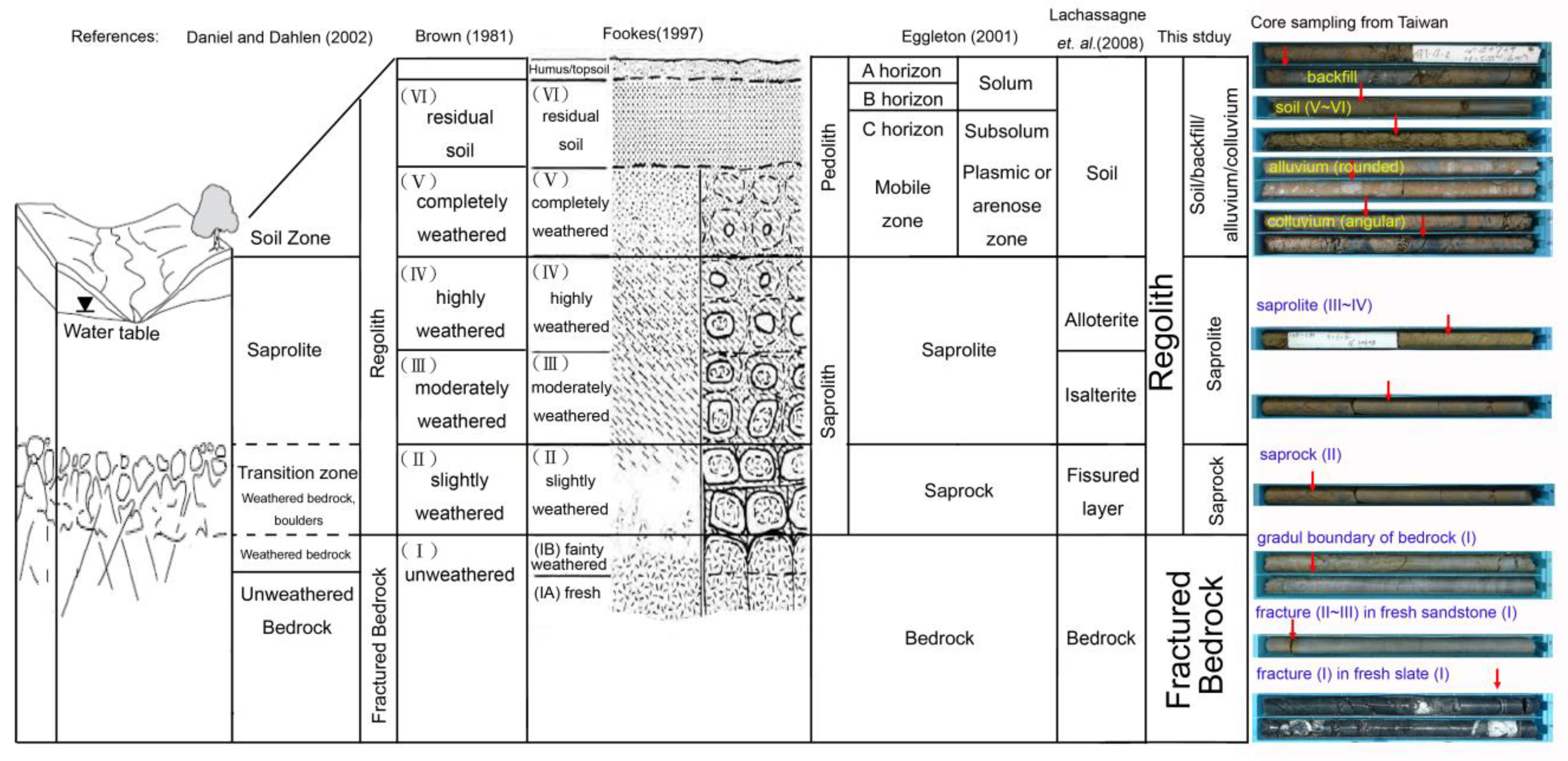
2.1. Regolith and Fractured Bedrock

According to the hydrogeological conceptual model (Figure 1), there are two major layers (i.e., regolith and fractured bedrock) in the mountainous regions. Regolith materials overlaid on bedrock are defined by the conditions of weathering, from slightly weathered to residual soil [25,26]. The specific rock types are named in the literature [27,28,29]. In this study, the average depth of regolith was 15.9 m. There were three kinds of materials in the regolith layer inspected in 118 sites (100 m in depth) and samples. The first kind consists of soil, backfill, alluvium, and colluvium as inspected by the degree of weathering, sphericity, angularity, and roundness in Holocene. The other two kinds were saprolite and saprock, weathered from bedrock with the weathering between slight and high degrees, respectively. Faintly weathered and fresh bedrock belongs to fractured bedrock ranging from Eocene to Pleistocene.

The hydrogeological settings are mainly dominated by the lithological properties of the selected study area where porosity or secondary porosity (e.g., fracture) can provide space to store and trap water [30,31,32,33,34,35]. This information is included in the map of the hydrogeological unit to provide a conceptual hydrogeological model and characteristics [36,37,38,39].

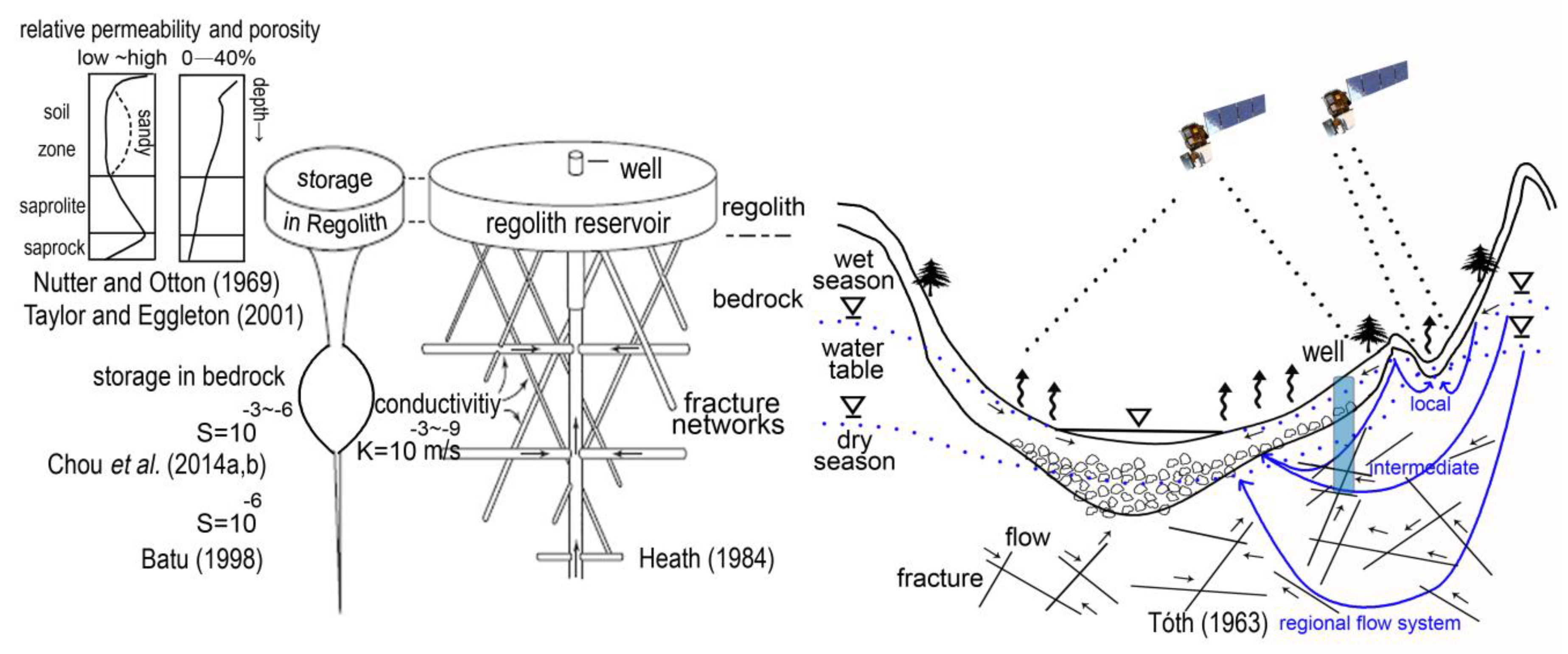
2.2. Hydrogeological Properties

In terms of experimental hydraulic parameters (Figure 2), the storage, permeability, and porosity of regolith are generally higher than those of bedrock [27,40,41,42]. However, groundwater in bedrock is distributed in fracture networks and tends to exist and flow at secondary weak planes or weathered zones with higher permeability [33,34,43,44,45].

The effects of surface topography on the groundwater flow system are described and simulated by theoretical and numerical methods [46,47]. There are three types of groundwater flow systems (i.e., local, intermediate, and regional flows) affected by topographic relief in a basin. Surface topography also generally reflects the spatial distribution of soil moisture and groundwater levels in the process of water infiltration, recharge, and discharge. The properties of SD, river gradient, flow accumulation (FA), drainage density (DD), and TWI can be analyzed from a DEM. The regional geomorphology, land cover or land use, groundwater recharge, and water bodies can be determined by ground investigation or derived from RS [48,49,50,51,52]. Furthermore, geological lineament structures provide information on regional connectivity of a fracture network, where the groundwater potential could be higher [53,54,55]; in addition, spatiotemporal land surface temperature (LST), normalized difference vegetation index (NDVI), and soil moisture index (SMI) provide dynamic evidence on groundwater recharge and discharge [56,57,58].

Therefore, hydrogeological characteristics change with the evolution of regional geology and topography. The target of groundwater exploration in this study was discharge areas that are composed of regolith and fractured bedrock aquifers. It becomes feasible to determine remotely sensed surface characteristics linked to groundwater by using the proposed RS and GIS model.

3. Materials and Method

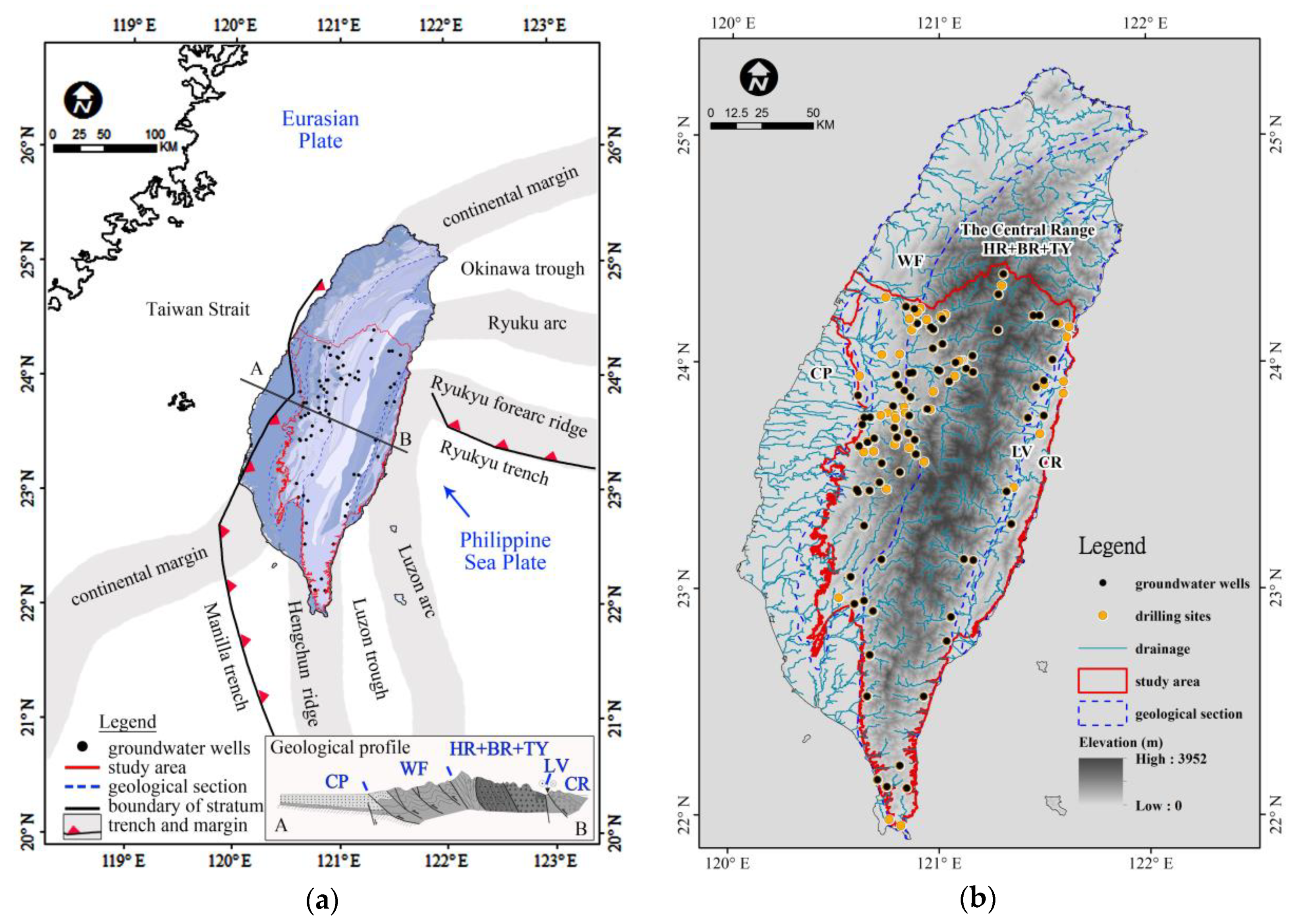
3.1. The Study Area

The island of Taiwan (Figure 3) covers an area of 35,873 km², and its central geographic coordinates are 23°58′ N and 120°58′ E. In Taiwan, 25 central government-governed rivers originate in the steep topography, which has an elevation ranging from sea level to 3952 m. The island is 394 km long and 144 km wide. The geological sections [7,59] from east to west are delineated by major tectonic structures and faults, including the Coastal Range (CR), Longitudinal Valley (LV), Taroko and Yuli Belt (TY) of the East Central Range, the Hsueshan Range (HS) and the Backbone Range (BR) of the West Central Range, the Western Foothills (WF), and the Coastal Plain (CP). In the evolution of plate tectonics in Taiwan, the Tananao Schist complex is composed of a metamorphic pre-Tertiary basement of the Eurasian passive margin, which has evidence of past orogenic events in recent metamorphic events. For instance, the TY belt was strongly deformed and metamorphosed in the Mesozoic period. Due to the Cenozoic arc-continent collision and orogeny located on the boundary of Eurasia and the Philippines Sea plates, the slate belt in the HS and BR is connected with the Chinese passive continental margin, the CR corresponds to the accreted Luzon arc, and the LV is considered a suture zone between the arc and continental margin. In the western foreland basin, the WF at lower altitudes has been accreted and deformed with syn-orogenic sediments, and the CP is part of the present foreland basin. As a result of this orogenic movement, the terrain of Taiwan consists of approximately 1/3 plains and 2/3 mountain regions (Figure 3). The plain areas (e.g., CP and LV), where the formations of unconsolidated rocks are divided into aquifers and aquitards according to the hydrogeological characteristics, are delineated into 9 major groundwater areas and are the locations of most of the major cities. In the mountain regions (e.g., WF, HS, BR, TY and CR), the formation of consolidated rock mainly includes sedimentary, metamorphic, and volcanic rocks ranging from Eocene to Pleistocene with complex fracture networks of folds and faults.

Due to the limited number of investigations to date, the central and southern mountainous regions of Taiwan were chosen as the study area. The area is about 19,098 km² in size, and it is 280 km long and 110 km wide. The eastern and western watersheds originate from the Central Range, below the elevation of 3952 m, and include 11 rivers: the Dajia, Wu, Jhuoshuei, Pachang, Zengwun, Gaoping, Sizhong, Hoping, Hualien, Xiuguluan, and Beinan rivers. The 118 drilling sites and 72 groundwater wells were distributed in different topographic terrains and in each geological section of the WF, HR, BR, TY, and CR, as shown in Figure 3.

3.2. Materials

The primary data used in this study consist of:

(1)

A digital geological map with a scale of 1:25,000 established by the Central Geological Survey (CGS), including distributions of geological formations, faults, and folds.

(2)

DEM with a resolution of 30 m × 30 m provided by the Advanced Spaceborne Thermal Emission and Reflection Radiometer Global Digital Elevation Model (ASTER GDEM).

(3)

Remotely sensed Landsat imagery captured on 6 November 1994; 9 June and 2 December 2015; and 27 June and 4 December 2016.

(4)

118 drilling samplings (100 m in depth) and well yield data analyzed from 72 pumping tests (40 m in average depth) were implemented by the CGS and Sinotech Engineering Consultants, incorporated.

(5)

Post-processing production:

(a)

Landsat imagery

• The image of first plane of principal component (PC-1) derived from principal component analysis (PCA) on 6 November 1994.
• Map of lineaments greater than 1 km in length extracted by the LINE module of PCI Geomatica.
• LST, NDVI, and SMI maps calculated from the function of Band Math in ENVI.

(b)

DEM

• SD, FA, TWI, and TPI maps analyzed from the function of Raster Calculator in ArcGIS.
• The major drainage in each watershed was extracted by a threshold value of FA.

(c)

HGU map delineated from the geological map.

(d)

Density map of lineament density (LD) and DD analyzed from the function of line density in ArcGIS.

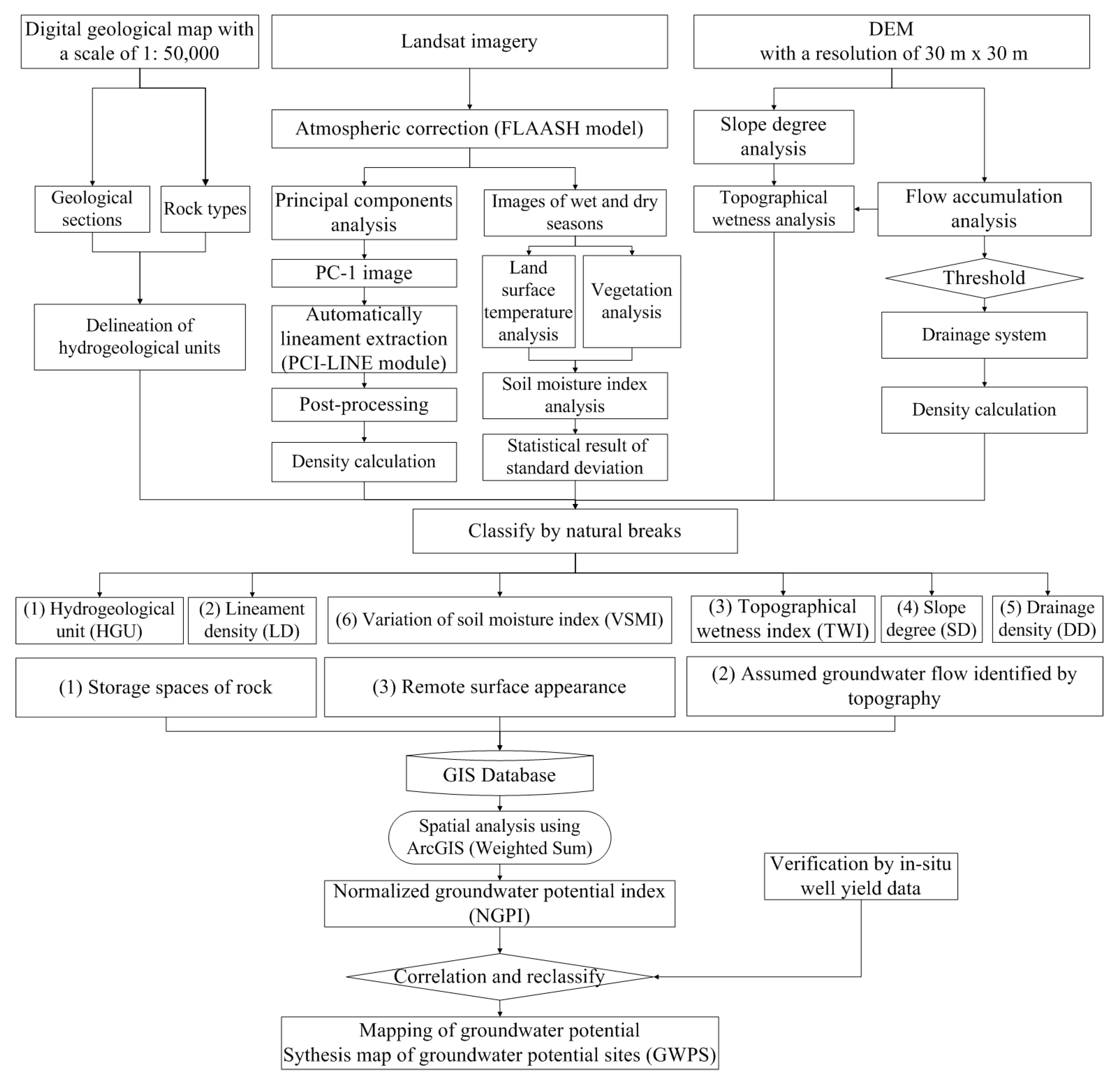
3.3. Methodology

To achieve the goal of cost-effective groundwater exploration and recognize the influence of the likely parameters on the ACC, the unique features related to groundwater potential were configured and described by integrating RS and GIS techniques with favorable groundwater parameters in the same spatial resolution of 30 m × 30 m, including lineaments and SMI derived from Landsat imagery, and SD, DD, and TWI analyzed from DEM. HGU was considered as the parameter of lithology to simultaneously reflect the complex spatial distribution of geological structures and rock types in the ACC. Therefore, six specific parameters, namely, HGU, LD, SD, DD, TWI, and a variation of the SMI (VSMI) were selected to compute the NGPI in the ArcGIS Spatial Analyst module using Equation (1). The values of ranking and weight may change in each case study. To avoid the subjective effect on each parameter, its equal weight and appropriate 5 classifications of ranking were used in this study. That is, the weighting of each parameter was designed to be the same value of 1. In addition, the ranking of each parameter was based on the low to high groundwater potential and computed by the scale value of 0–5. Except for the parameter of HGU, the data formats of the other 5 parameters were digital numbers to determine the best arrangement of values by Jenks Natural Breaks (JNB) classification method [60,61] into 5 designed rankings. Therefore, it is helpful to understand the groundwater potential of each selected parameter in the RS-GIS model. Finally, the NGPI with 6 proposed parameters in each pixel was computed with the values of 0–30 and normalized from 0 to 1 in the final synthesized map of groundwater potential. The results were evaluated according to in-situ well yield data from 72 wells.

$$\mathrm{NGPI}=\frac{{{\displaystyle \sum }}_{\mathrm{i}=1}^{\mathrm{i}=6}{\mathrm{P}}_{\mathrm{i}}{\mathrm{X}\mathrm{W}}_{\mathrm{i}}}{{{\displaystyle \sum }}_{\mathrm{i}=1}^{\mathrm{i}=6}{\mathrm{P}}_{\mathrm{i}\max }{\mathrm{X}\mathrm{W}}_{\mathrm{i}}}$$

(1)

where P_i is the ranking of each parameter given by the scale value of 0–5, and W_i is the weight of each parameter given by the same value of 1 in this study.

As illustrated in the study framework in Figure 4, the selected parameters and products include: (1) generating a geological map with a scale of 1:25,000 established by the CGS and delineating HGUs to complete the post-produced hydrogeological map; (2) deriving LD and multiple temporal SMI from Landsat imagery; and (3) analyzing DEM to calculate SD, DD, and TWI. The processing of the parameters (

Table 2. Ranking and value of each parameter and its benefit to groundwater prospect.

Parameters 1		Benefit to Groundwater Prospect
(a) HGUs		Geological section (i)	Main rock type (ii)	Ranking (i + ii)
1	UCRK	CP and LV section as well as those with unconsolidated rock, such as alluvium and river terrace.		5
2	WFGR	WF (1)	Gravel (2)	3
3	WFSM		Mud (1)	1
4	WFSS		Sandstone and shale (2)	3
5	WFSH		Shale (0)	1
6	HRAR	HR (2)	Argillite (0)	2
7	HRQS		Quartz (2)	4
8	HRSA		Sandstone and slate (2)	4
9	HRSL		Slate (2)	4
10	BRSP	BR (2)	Phyllite (2)	4
11	TYSC	TY (2)	Schist (2)	4
12	TYGN		Gneiss (2)	4
13	TYMB		Marble (0)	2
14	CRMS	CR (1)	Mud (1)	2
15	CRGR		Gravel (2)	3
16	CRSS		Sandstone and shale (2)	3
17	CRBR		Volcanic breccias (2)	3
(b) LD (km/km2) classified by Jenks Natural Breaks			Fracture network	Ranking
1	0.576~1.045		Well-developed	5
2	0.448~0.576		High	4
3	0.321~0.448		Medium	3
4	0.165~0.321		Low	2
5	0.000~0.165		Intact rocks	1
(c) SD classified by Jenks Natural Breaks			Predominated terrain	Ranking
1	0~10		Flat terrain, riverbed, thicker regolith	5
2	10~22		Gentle flat slope	4
3	22~32		Flat slope	3
4	32~42		Steep slope	2
5	42~83		Steep slope with more runoff	1
(d) DD (km/km2) classified by Jenks Natural Breaks			Drainage system and development	Ranking
1	0.000~0.143		Fewer drainage, favorable to recharge	5
2	0.143~0.213		Slightly	4
3	0.213~0.285		Medium	3
4	0.285~0.374		Highly	2
5	0.374~0.596		More drainage and erosion	1
(e) TWI (m/m2) classified by Jenks Natural Breaks			Runoff and comparative wetness	Ranking
1	4.17~11.41		Downstream, more flow accumulation (FA), thicker regolith	5
2	2.54~4.17		Main river	4
3	1.43~2.54		Branch, creek	3
4	0.62~1.43		Upstream, slop flow	2
5	0.00~0.62		Roof, steep slope area	1
(f) VSMI classified by Jenks Natural Breaks			Variation of soil moisture and recharge	Ranking
1	1.11~5.29		Severe potential	5
2	0.61~1.11		High potential	4
3	0.38~0.61		Medium potential	3
4	0.23~0.38		Slight potential	2
5	0.00~0.23		Lower potential	1

¹ The proposed six parameters were hydrogeological units (HGUs), lineament density (LD), slope degree (SD), drainage density (DD), topographic wetness index (TWI), and variation of the soil moisture index (VSMI), After assigning the ranking of HGUs in the vector format, they were reclassified as a raster format. The other data formats were digital numbers to determine the best arrangement of values by Jenks Natural Breaks classification method [60,61] into 5 designed rankings.

and Figure 5) and in-situ well yield data are introduced in Appendix A.

4. Results

According to the method described, six group variables, namely, HGU, LD, SD, DD, TWI, and VSMI (Figure 5), were computed in the RS-GIS model. The final synthesized map with NGPI was produced. In addition, the correlations between groundwater potential, NGPI, and the findings are described below.

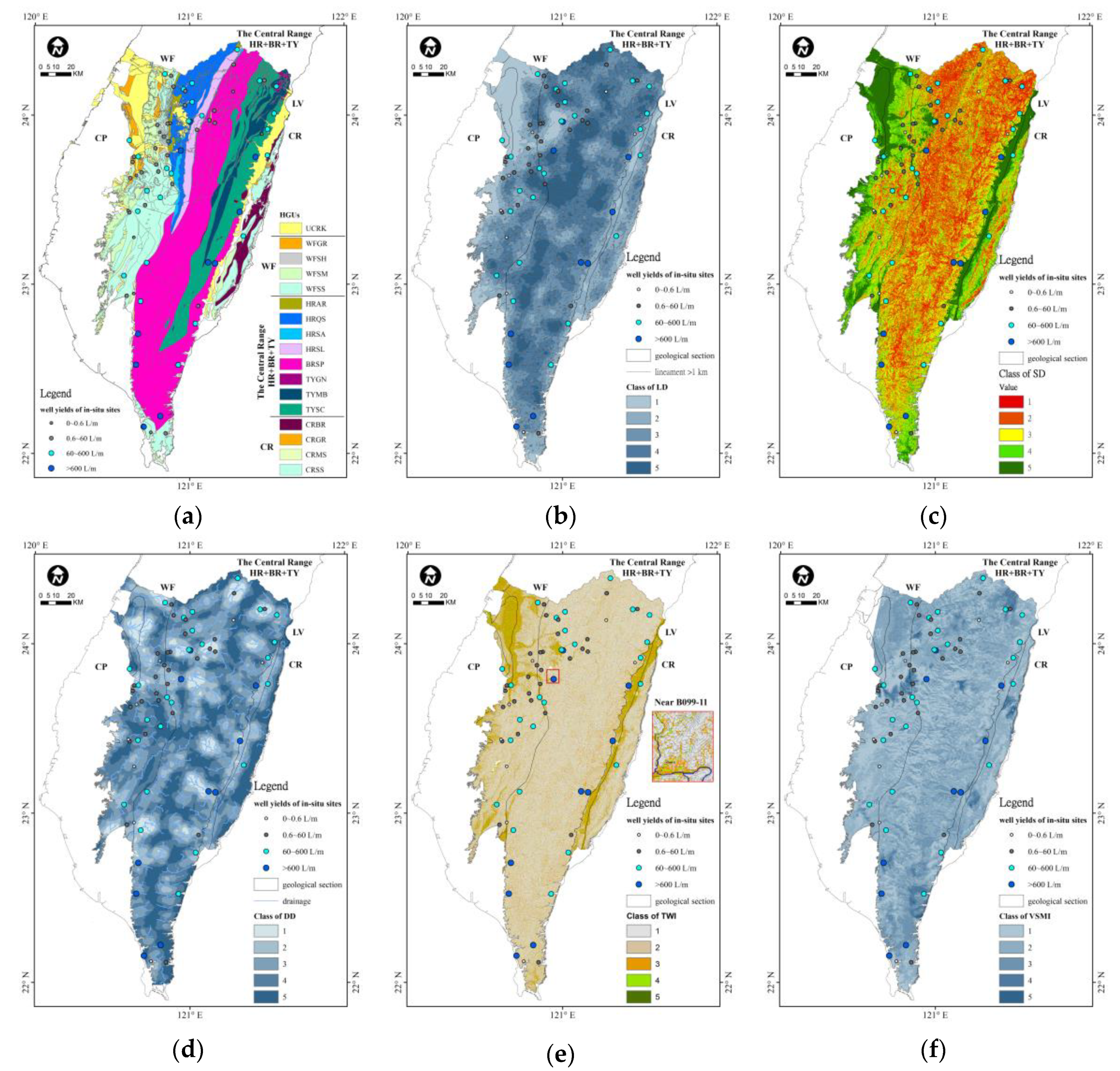
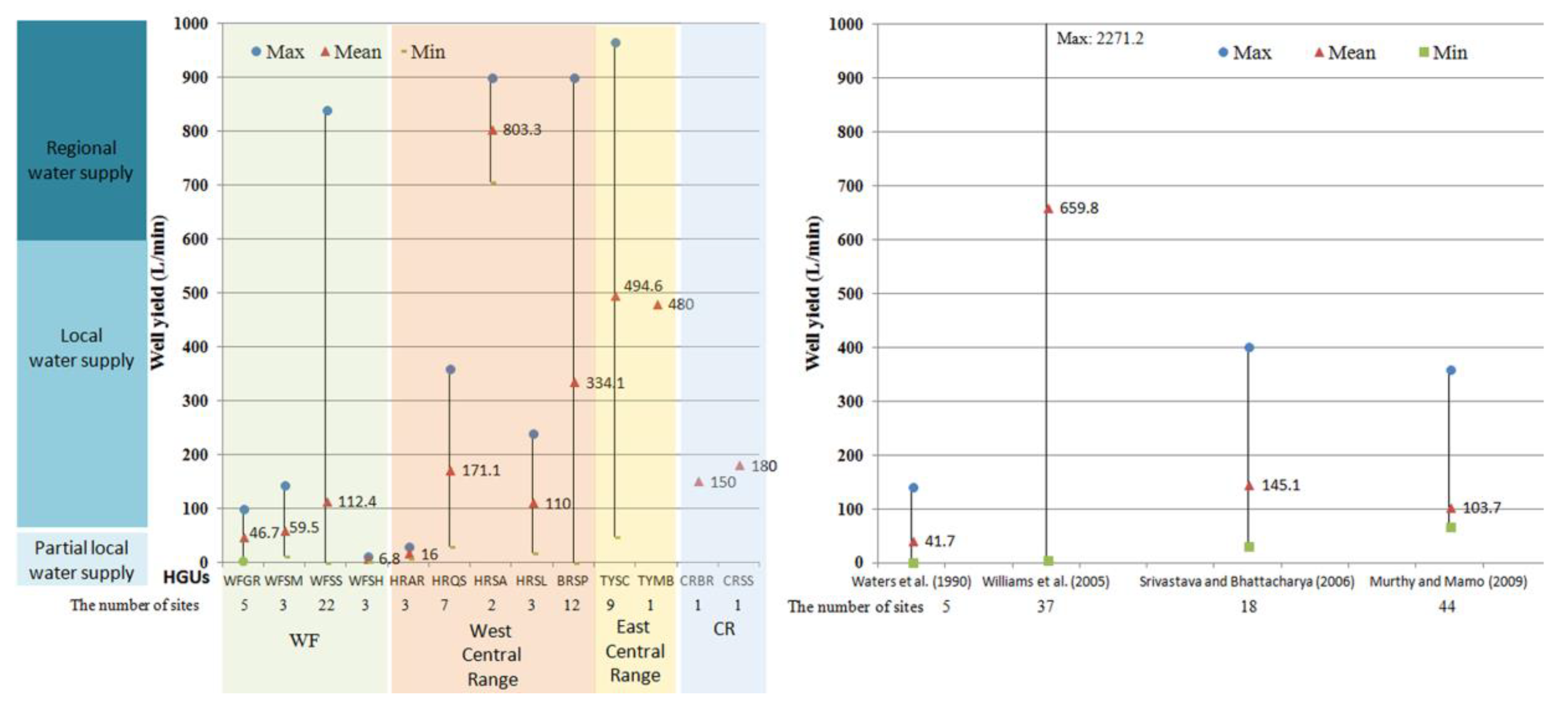
4.1. HGU Thematic Map and Distribution of Well Yields

Delineation of HGUs is a primary task of hydrogeological investigations. For each case of an HGU thematic map, the information depends on the scale and purpose of the study. In the ACC of Taiwan, delineation of HGUs by geological sections and rock types simplified the complex geological units into 17 HGUs and provided the general geological and hydraulic properties. In addition, limited in-situ investigation in each HGU outlined the groundwater potential, as shown in Figure 6. The 72 wells investigated were located in the WF, the Central Range, and CR. Results showed that most average well yields of the HGUs belonged to WFSS in the Western Foothills, and HRQS, HRSA, HRSL, BRSP, and TYSC in the Central Range. However, the HGUs of WFSS, BRSP, and TYSC had large variability in their well yield values as well as the lithologic units in the Lawrenceville of Georgia [62]. Other dominant factors also control groundwater potential, such as fracture and geomorphology [7,12]. In contrast, WFSH and HRAR had lower groundwater potential due to the composition being mostly mud and less-fractured; consistently the well yield of 30 L per minute was distributed in the shale and slate [20]. This finding strongly supports the correct delineation and ranking of HGUs in the ACC. The trend of groundwater potential provided the primary information and references for the candidates of water supply.

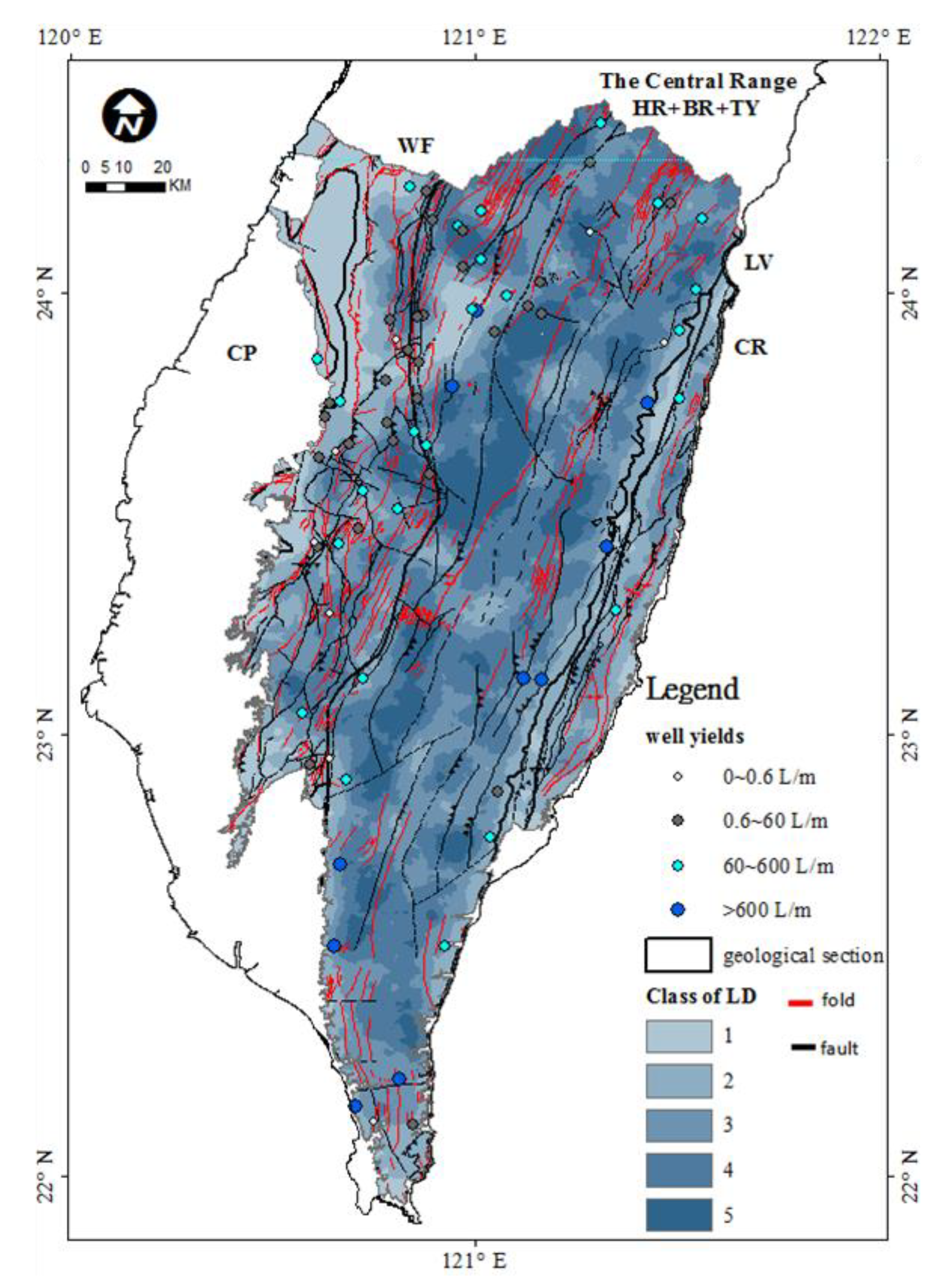
4.2. LD Thematic Map

Tectonic movement may cause numerous weak planes, fractures, and lineaments near the geological structures of faults and folds. In the LD thematic map (Figure 7), fault and fold lines were distributed around the areas with high LD, such as near the boundary of the WF and Central Range, the east part of the Central Range, and the middle of the CR. These results indicated that the given parameters of lineament extraction in the PCI-LINE module were appropriate. The values of RADI, GTHR, LTHR, FTHR, ATHR, and DTHR were tested and adjusted according to a case study in the literature (

Table A1. Lists of parameter values of automatic lineament extraction, and literature.

Study Parameters	[54]	[55]	This Study
Radius of filter in pixels (RADI)	5	3	5
Threshold for edge gradient (GTHR)	10	30	15
Threshold for curve length (LTHR)	3	30	3
Threshold for line fitting error (FTHR)	3	5	3
Threshold for angular difference (ATHR)	7	30	10
Threshold for linking distance (DTHR)	3	30	10

). Linking the LD thematic map to groundwater potential, some in-situ sites with higher well yields were located in the areas with higher LD; however, some of those near the boundary of the WF and Central Range, where the rock types are deposited with more mud matrix, did not match the expected results. In the fold-bend fault region of the WF, the mud matrix of Miocene strata might fill the fracture space and block the groundwater flow from reaching connected fractures. Thus, a negative correlation was found between LD and groundwater potential in the WF of the ACC, and the local mud matrix should be considered and examined in future explorations, especially in the WF area.

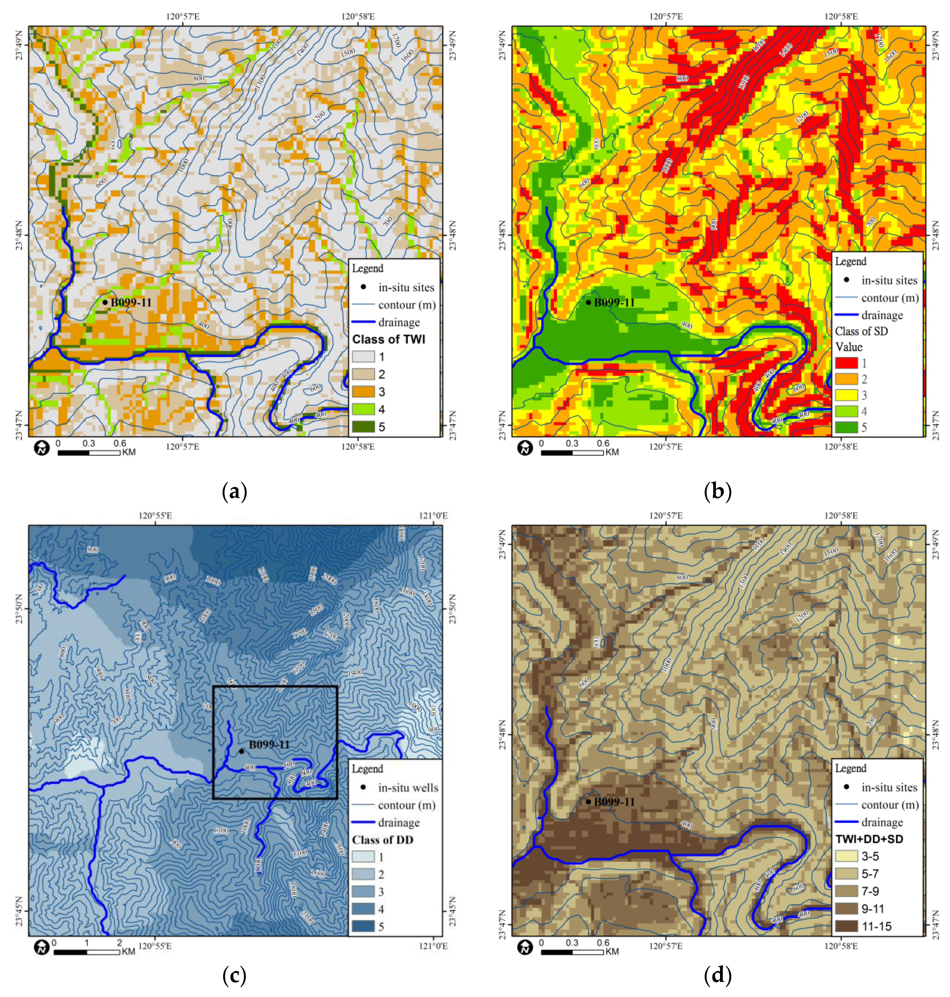
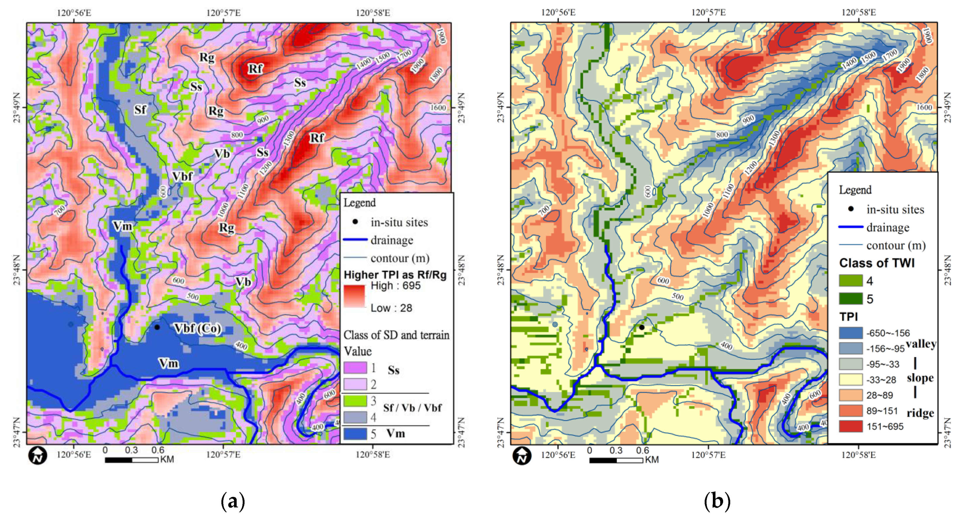
4.3. Geomorphic Thematic Map (TWI, SD, and DD)

Since groundwater may flow in accordance with variations of topography, the TWI is useful to describe the drainage system and runoff (Figure 8). Class 1 is distributed near the boundary of a watershed, class 2 belongs to slope flow, and class 3 is the downstream of slope flow. These flows may accumulate in the areas of classes 4 and 5, identified as streams and branches. The drainage calculated DD with the threshold of FA is distributed within classes 4 and 5 of the TWI. It helps to rank higher values in the sources of basins (i.e., lower DD) as the recharge areas on a regional scale. In addition, five classes of SD provide the general categories of terrain on a local scale. Therefore, the geomorphic thematic map was developed by overlaying the TWI, SD, and DD thematic maps to present preliminary information on groundwater occurrences.

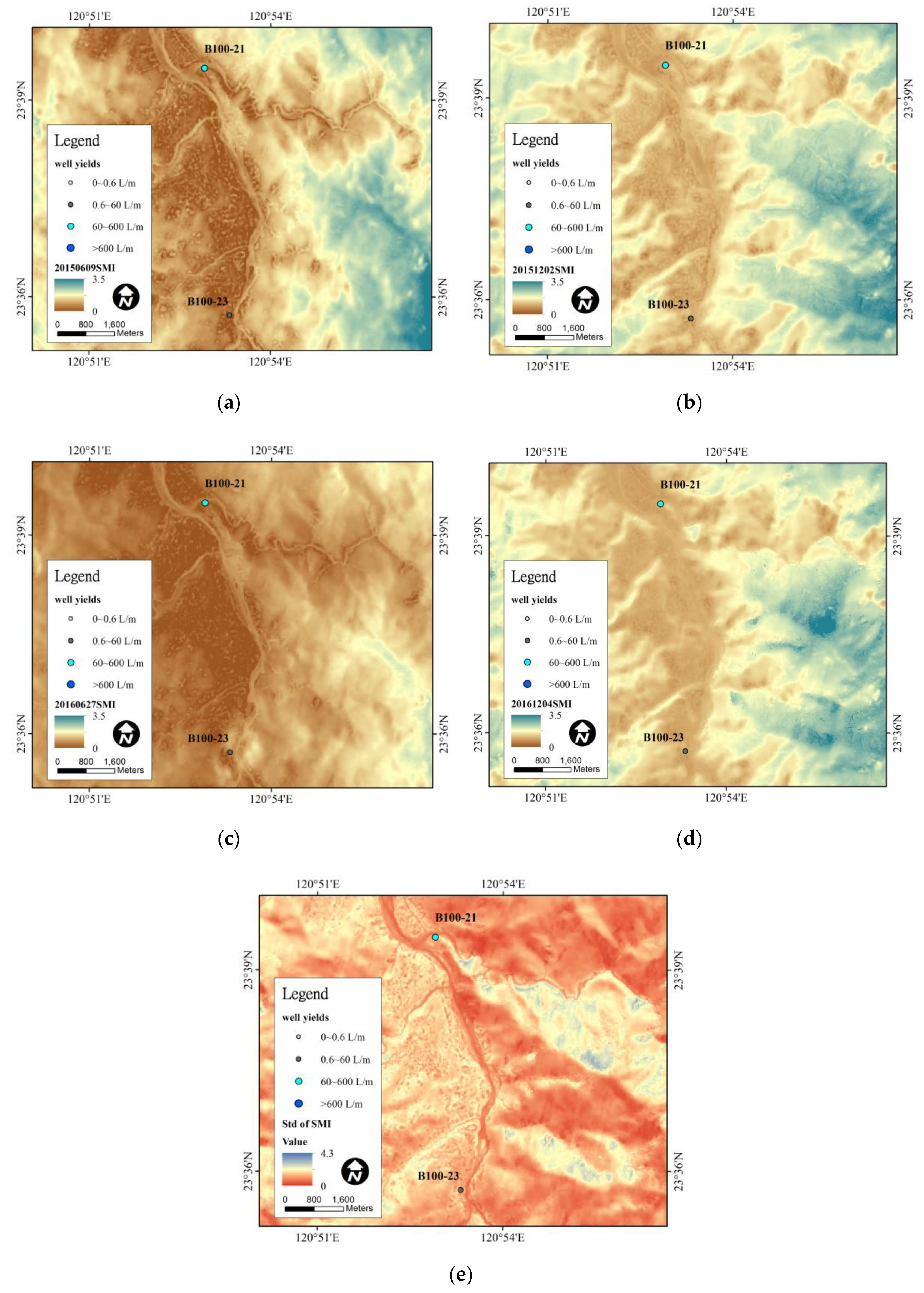
4.4. Seasonal SMI Thematic Map

To understand the correlation between the variation of soil moisture and groundwater potential, the SMI thematic maps of two wet and dry seasons and their standard deviation statistics were compared within the regions with different well yield levels (Figure 9). The results indicated that the seasonal trends in each year were similar, with the exception of specific regions, such as the B100-21 site. This site was located near a region with higher variation of SMI, and its well yield was comparatively higher than that of the B100-23 site. Therefore, SMI derived from Landsat was found to be a reliable source of information on groundwater potential.

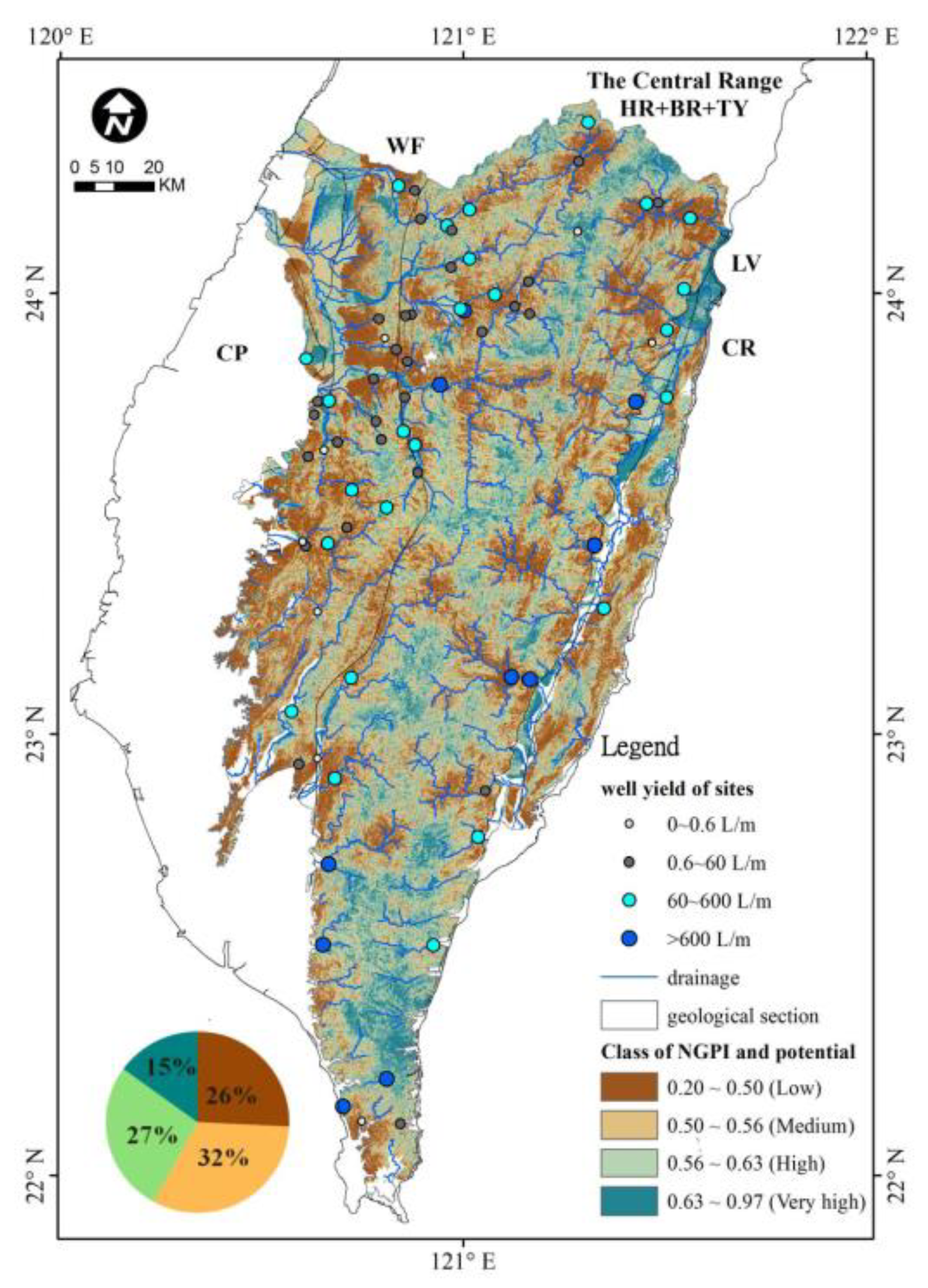
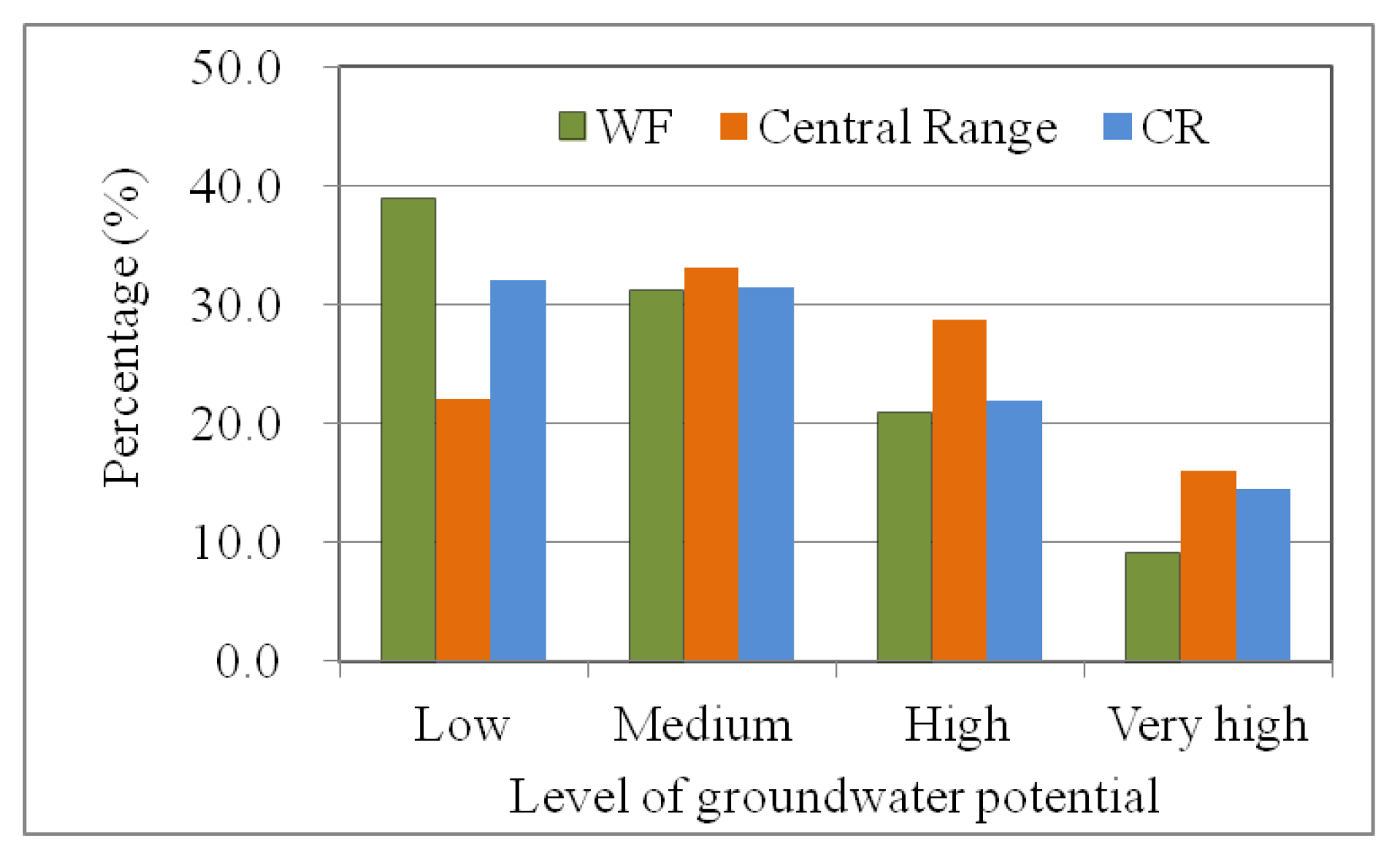
4.5. Mapping of Groundwater Potential

4.5.1. Classification of Groundwater Potential

In the above sections, all the selected parameters were discussed separately from well yields. Before mapping of groundwater potential, the four categories of GWPS (

Table 3. Classifications of groundwater potential and groundwater potential sites (GWPS) (after [63]).

Degree of Groundwater Potential	Well Yield (L/min)	Description	GWPS
High Potential	>600	Regional water supply for humans and irrigation	Yes
Medium Potential	60–600	Local water supply for humans and irrigation
Low Potential	0.6–60	Partial local water supply for personal use	No
Poor Potential	<0.6	Lack of water resources

) were defined by the values of well yields [63]. Groundwater sites with well yields of more than 600 L per minute are suitable as regional water supplies for humans and irrigation. Those with yields between 60 and 600 L per minute are considered local water supplies. Therefore, a GWPS is defined as having a well yield of greater than 60 L per minute; otherwise, it belongs to non-GWPS where groundwater is insufficient for water supply. According to the well yield data, the 72 groundwater sites were classified into two groups, GWPS and non-GWPS, as shown in

Table 4. Summarized characteristics of in-situ sites.

No.	Region	Site	Well Yield (L/min)	GWPS or Non-GWPS 1	Regolith Depth (m)	HGU	Terrain	NGPI
1	Central Taiwan	B099-15	22.8	non-GWPS	1.7	WFSM	Sf	0.43
2		B101-11	0.2	non-GWPS	15.2	WFSS	Vb	0.47
3		B099-02	8.08	non-GWPS	12.7	HRAR	Vb	0.47
4		B099-06	5.8	non-GWPS	9.4	WFSS	Vb	0.47
5		B099-09	11.85	non-GWPS	41.6	WFSH	Sf	0.47
6		B099-14	21.67	non-GWPS	8.6	WFGR	Rf	0.50
7		B100-15	0.9	non-GWPS	6.0	BRSP	Ss	0.50
8		B101-05	240	GWPS	7.7	HRSL	Vm	0.50
9		B102-07	0	non-GWPS	12.1	TYSC	Ss	0.50
10		B101-03	30	non-GWPS	43.2	HRQS	Ss	0.53
11		B102-02	48	non-GWPS	16.7	TYSC	Vb	0.53
12		B099-25	310	GWPS	17.5	WFSS	Sf	0.53
13		B100-16	42	non-GWPS	39.4	BRSP	Sf	0.53
14		B099-01	11.67	non-GWPS	8.3	WFSM	Vm	0.57
15		B099-03	62.76	GWPS	13.0	WFGR	Vm	0.57
16		B100-18	12	non-GWPS	30.0	BRSP	Vbf	0.57
17		B101-09	1.7	non-GWPS	12.2	WFSS	Sf	0.57
18		B101-10	0	non-GWPS	13.4	WFSS	Sf	0.57
19		B099-16	6.8	non-GWPS	17.8	WFSS	Sf	0.60
20		B099-29	32.4	non-GWPS	>100	WFSS	Vbf	0.60
21		B101-13	10	non-GWPS	6.6	HRAR	Vb	0.60
22		B100-03	2.75	non-GWPS	3.6	WFSS	Vb	0.60
23		B100-07	30	non-GWPS	47.0	HRAR	Vm	0.60
24		B100-17	36	non-GWPS	11.1	BRSP	Sf	0.60
25		B100-19	18	non-GWPS	4.0	HRSL	Vm	0.60
26		B101-12	6	non-GWPS	10.9	WFSS	Vm	0.60
27		B099-28	2.2	non-GWPS	5.4	WFGR	Vb	0.63
28		B101-14	240	GWPS	11.6	HRQS	Sf	0.63
29		B101-15	900	GWPS	7.5	HRSA	Vm	0.63
30		B102-01	90	GWPS	13.1	TYSC	Vb	0.63
31		B102-09	150	GWPS	2.1	CRBR	Vm	0.63
32		B099-11	706.67	GWPS	50.2	HRSA	Vbf	0.67
33		B099-19	88.3	GWPS	20.0	WFSS	Sf	0.67
34		B100-02	240	GWPS	18.4	WFSM	Vm	0.67
35		B100-08	125	GWPS	10.9	HRQS	Vm	0.67
36		B099-21	106.94	GWPS	14.5	HRQS	Vm	0.67
37		B099-23	40	non-GWPS	11.7	WFSS	Vm	0.67
38		B100-11	36	non-GWPS	7.8	HRQS	Vb	0.67
39		B102-06	420	GWPS	68.4	TYSC	Vm	0.67
40		B099-17	0.6	non-GWPS	5.4	WFSS	Vbf	0.70
41		B100-13	72	GWPS	5.2	HRSL	Vm	0.70
42		B102-05	240	GWPS	14.6	TYSC	Vm	0.70
43		B100-10	300	GWPS	22.1	HRQS	Sf	0.70
44		B101-06	0.6	non-GWPS	0.5	BRSP	Vb	0.70
45		B102-03	480	GWPS	15.7	TYMB	Vbf	0.70
46		B102-08	780	GWPS	10.8	TYSC	Vbf	0.70
47		B101-04	360	GWPS	9.8	HRQS	Vbf	0.73
48		B101-08	100	GWPS	8.0	WFGR	Vbf	0.73
49	Southern Taiwan	B104-05	0	non-GWPS	5.6	WFGR	Vb	0.43
50		B104-04	17.5	non-GWPS	4.6	WFSS	Sf	0.47
51		B105-07	0	non-GWPS	7.3	WFSS	Sf	0.50
52		B106-03	180	GWPS	12	CRSS	Sf	0.50
53		B106-06	1.8	non-GWPS	3.7	BRSP	Vm	0.50
54		B105-05	0	non-GWPS	6.8	WFSS	Vb	0.53
55		B105-06	40	non-GWPS	9.8	WFSS	Vb	0.53
56		B104-02	150	GWPS	4.5	WFSS	Sf	0.53
57		B105-03	8	non-GWPS	16.1	WFSS	Vb	0.57
58		B105-04	350	GWPS	30.9	WFSS	Sf	0.57
59		B103-06	0	non-GWPS	8	WFSH	Vbf	0.60
60		B103-07	1.8	non-GWPS	6.35	WFSH	Sf	0.60
61		B104-06	298	GWPS	3.2	BRSP	Vm	0.63
62		B106-02	966	GWPS	42.7	TYSC	Vm	0.63
63		B106-04	750	GWPS	12.3	TYSC	Vm	0.63
64		B104-01	195	GWPS	12.7	WFSS	Vm	0.63
65		B106-05	663	GWPS	34.1	TYSC	Vm	0.63
66		B104-07	738	GWPS	45	BRSP	Vm	0.67
67		B105-01	153	GWPS	15	WFSS	Sf	0.70
68		B103-05	840	GWPS	7.5	WFSS	Vbf	0.70
69		B103-01	840	GWPS	32.2	BRSP	Vm	0.73
70		B103-02	900	GWPS	31.7	BRSP	Vm	0.73
71		B103-03	300	GWPS	25.9	BRSP	Vbf	0.73
72		B103-04	840	GWPS	5.2	BRSP	Vm	0.77
Average value			203.9	-	15.9	-	-	0.60

¹ A GWPS is defined as having a well yield of greater than 60 L per minute; otherwise, it belongs to non-GWPS where groundwater is insufficient for water supply. Abbreviations: near roof (Rf), at ridge (Rg), steep slope (Ss), flat slope (Sf), valley or creek bottom (Vb), alluvial fan of downstream the valley (Vbf), main riverbed deposit (Vm).

, whose percentages were 48.6% and 51.4%, respectively.

4.5.2. Final Synthesized Map of Groundwater Potential in the ACC

The resulting synthesized map of groundwater potential is shown in Figure 10. NGPI values were classified into four levels by JNB as low (0.20~0.50 NGPI), medium (0.25~0.56 NGPI), high (0.56~0.63 NGPI), and very high (0.63~0.97 NGPI) groundwater potential. The percentages of the low, medium, high, and very high potentials were 26%, 32%, 27%, and 15%, respectively. NGPI values, which range from 0 to 1, were compared with the well yield data, as shown in Table 4. There was a positive correlation between the NGPI and well yields.

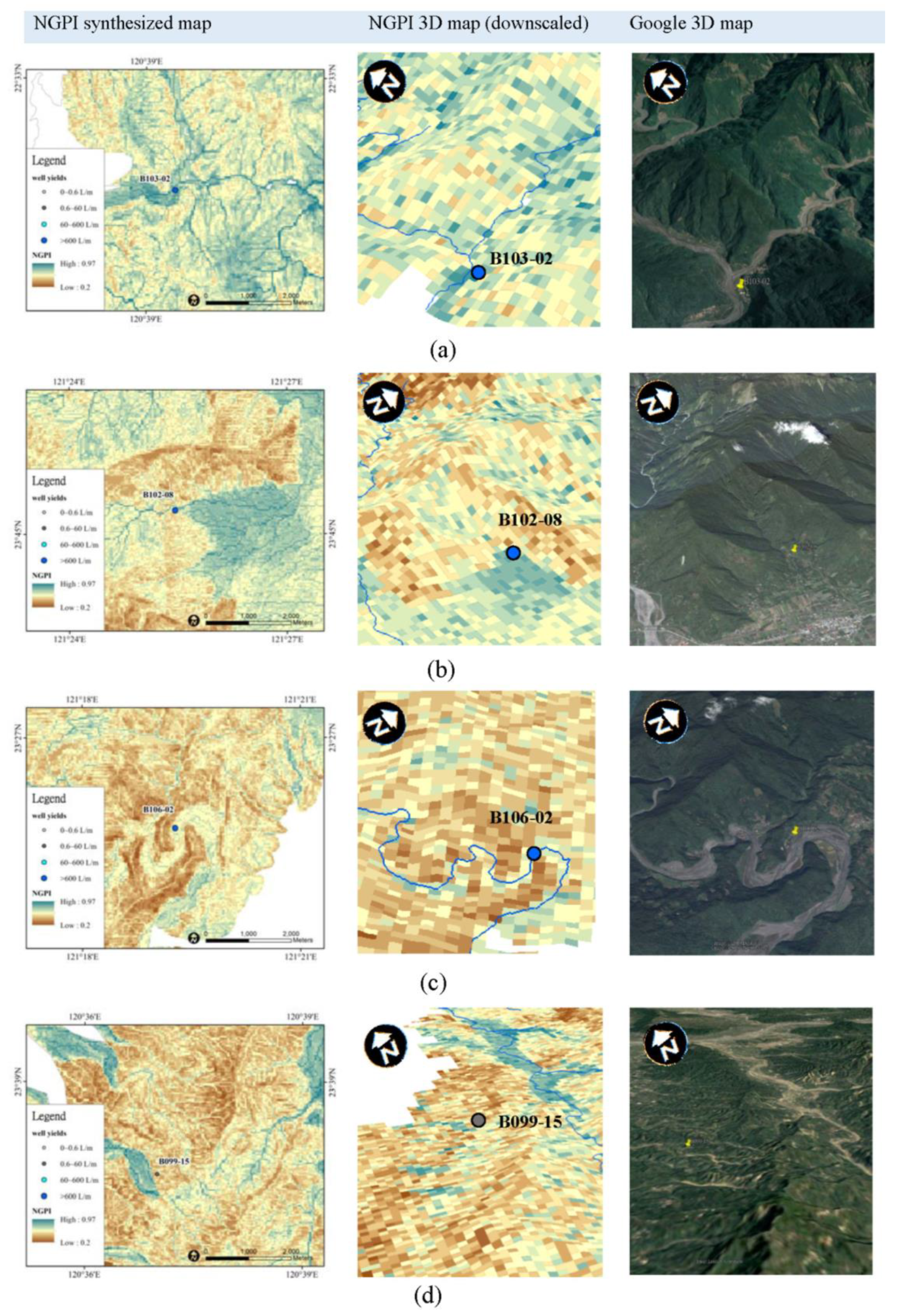
4.5.3. Application of the NGPI to Predict Groundwater Potential and Verification of In-Situ Data

Since the very high level of NGPI was above 0.63, the threshold of the NGPI for identifying GWPS and non-GWPS was determined to be 0.63. To apply and inspect the NGPI for groundwater exploration, the well yield data of 48 sites in central Taiwan were employed as training data. The value achieved an accuracy of 83.3%. According to previous experience, 24 sites in southern Taiwan were predicted. The estimated results achieved an accuracy of 87.5%, while that for all the tested sites was 84.7% (

Table 5. Statistical results of NGPI, well yield, GWPS, and non-GWPS.

Region	NGPI	Well Yield (L/min)	Number of Sites (Predicted)	Number of Sites (Actual)	Accuracy (%)	Total (%)
Central Taiwan	≥0.63	≥60 (GWPS)	22	17	77.3	83.3
(Training data)	<0.63	<60 (non-GWPS)	26	23	88.5
Southern Taiwan	≥0.63	≥60 (GWPS)	12	12	100	87.5
(Predicted results)	<0.63	<60(non-GWPS)	12	09	75.0
Whole study area	≥0.63	≥60 (GWPS)	34	29	85.3	84.7 *
(>60 L/min as GWPS)	<0.63	<60 (non-GWPS)	38	32	84.2
Whole study area	≥0.63	≥300 (GWPS)	34	14	41.2	69.4
(>300 L/min as GWPS)	<0.63	<300 (non-GWPS)	38	36	94.7
Whole study area	≥0.63	≥600 (GWPS)	34	11	32.4	68.1
(>600 L/min as GWPS)	<0.63	<600 (non-GWPS)	38	38	100

* The prediction accuracy of all the tested sites to identify GWPS with well yields exceeding 60 L per minute was about 84.7%. Thus, the reliability of the synthesized map of NGPI was improved.

). On the other hand, using a threshold of 0.63 to predict more well yields (higher than 300 or 600 L per minute) as GWPS resulted in lower accuracy. Therefore, the definitions of GWPS were met by the degree of 0.63~0.97 NGPI (very high) and verified with in-situ data. The verified NGPI value of 0.63 is a significant threshold for identifying local and regional water supplies in the follow-up groundwater exploration in the ACC.

5. Discussion

5.1. Proposed Parameters of Spatial Resolution

Although GIS spatial analyst tool provides the fast result of a thematic map of weighted sum with proposed parameters, the result may be less useful due to the inconsistency of data sources and spatial resolution. However, the use of a finer grid for pointwise exploration is expensive and may still not be able to determine in areas where traffic cannot be reached. Under the issue of achieving the goal of a cost-effective method in remote areas by integrating RS and GIS techniques, the global Landsat imagery and ASTER GDEM can be obtained from the National Aeronautics and Space Administration (NASA) website with a uniform spatial resolution of 30 m × 30 m. The proposed parameters can be produced from the raw data. Thus, a raster-based empirical GIS model is recommended to calculate the thematic map of groundwater potential and validate it with investigated data.

5.2. Geologically Complex Terrain

5.2.1. Geological Characteristic of Groundwater Potential

For inspection of the possibility of groundwater potential in each geological section and rock type,

Table 6. Statistics of percentages of GWPS in the category of geological section and rock type.

Category		Number of Sites	Number of GWPS	Percentage (%)
(1) Geological section	The Central Range (HR, BR, TY)	37	23	62.2
	WF	33	10	30.3
	CR	2	2	*
(2) Rock type	Slate (HRSA, HRSL)	5	4	80.0
	Schist (TYSC)	9	7	77.8
	Quartz (HRQS)	7	5	71.4
	Phyllite (BRSP)	12	6	50.0
	Gravel (WFGR)	5	2	40.0
	Sandstone and shale (WFSS, CRSS)	23	8	34.8
	Mud, shale, argillite (WFSM, WFSH, HRAR)	9	1	11.1
	Marble, volcanic breccias (TYMB, CRBR)	2	2	*

* No statistics due to insufficient data.

shows the percentage of GWPS at investigated sites. The geological section of the Central Range (e.g., HR, BR, and TY) is mostly composed of metamorphic rock (e.g., slate, schist, phyllite, and quartz) with a higher groundwater potential than that of WF (e.g., alternations of sandstone and shale). For the rock types of mud, shale, and argillite, the ingredients of very fine sand and mud caused the frequency of groundwater potential to be lower, whether they belonged to metamorphic rock or not. In addition, the percentages of medium, high, and very high levels of groundwater potentials in each geological section were higher in the Central Range (Figure 11). These findings correspond to the high possibility of GWPS in the metamorphic rock of the ACC (Figure 6). Thus, appropriate rankings and selected parameters of HGU and LD are sufficient to support the information on fracture networks affecting the groundwater potential in the active ACC area of Taiwan.

5.2.2. Topographic Characteristic of Groundwater Potential

Revised from a previous study [64], the seven categories of terrain are defined as near roof (Rf), at ridge (Rg), steep slope (Ss), flat slope (Sf), valley or creek bottom (Vb), alluvial fan of downstream the valley (Vbf), and main riverbed deposit (Vm), as shown in

Table 7. Statistics of regolith depth and GWPS in delineated terrain.

Terrains in the Mountainous Region		Definition	Average Regolith Depth (m)	Number of Sites	Number of GWPS	Percentage (%) in Each Terrain
Ridge of watershed	(1) Near roof (Rf)	TPI ≥ 28	*	1	0	*
	(2) At ridge (Rg)	TPI ≥ 28	N.A.	N.A.	N.A.	N.A.
2. 2. Slope area	(3) Steep slope above 32° (Ss)	Class 1 and 2 of SD	*	3.	0.	*
	(4) Flat slope under 32° (Sf)	Class 3 and 4 of SD	16.1	18	8	44.4
3. Valley and alluvial fan	(5) Creek bottom (Vb)	Class 3 and 4 of SD, and class 4 of TWI	9.2	14	1	7.1
	(6) Alluvial fan downstream Vb (Vbf)	Class 3 and 4 of SD, and class 4 of TWI	17.1	11	7	63.6
	(7) Main riverbed deposit and terrace (Vm)	Class 5 of SD and class 5 of TWI	18.7	25	19	76.0
Total			15.9	72	35	48.6

* No statistics due to insufficient data; N.A.: not applicable.

. To illustrate those terrains, the TPI, TWI, and SD were implemented. As for SD, classes 1 and 2 belong to Ss, classes 3 and 4 represent Sf, Vb, and Vbf, and class 5 is Vm. Furthermore, Vb and Vbf can be extracted by the class 4 of TWI. Finally, the topography tool of ArcGIS was used to derive the TPI and delineate the geomorphic terrain from ridge to valley (Figure 12) where the areas with TPI values above 28 were defined as Rf and Rg.

Within the data from the 72 investigated wells, less data on the Rf, Rg, and Ss terrains were available due to the difficulty of drilling and testing. The lower well yields may be located in those terrains as well as Vb. However, other terrains with higher percentage of GWPS included Vm, Vbf, and Sf, the average regolith depths of which were thicker in sequence. In addition, there was a positive correlation between regolith depth and well yield. Thus, for groundwater exploration based on topographic characteristics, the possibility of GWPS was about 44.4% to 76% (Table 7). With integration of RS and GIS, the possibility increased to 84.7% (Table 5). Therefore, another key parameter of GWPS is the characteristics of geology and remote sensing index (e.g., the proposed parameters of HGUs, LD, and VSMI in this study).

5.3. Visualization of the NGPI to Identify Groundwater Potential

The visualization of three-dimensional (3D) results provides information about potential sites [65]. However, in agricultural eras preceding modern computer analysis, people relied on the characteristics of terrain and their personal experience of groundwater exploration. For instance, the Chinese proverbs related to the locations of GWPS describe the confluences of two rivers, intersections of two mountains, concave sides of riverbeds at the foot of mountains, and so on. It is not easy to understand these descriptions of groundwater potential from the ancient proverbs without comparing the 3D visualization of the NGPI map with a Google map (Figure 13 and Figure 14). At site B103-02, the distribution of higher NGPI values shows a pattern consistent with the confluence of two upstream rivers. Site B102-08, located in a downstream deposited alluvial fan, is shaped into the mouth where two mountains intersect, and is also illustrated by a higher NGPI value. Site B106-02, located on meandering terrain and the concave side of a riverbed, is full of groundwater due to reduction of the flow velocity and increases in recharged water resources. Those predominant types of terrain are favorable to GWPS. Oppositely, an area composed of nearly horizontal bedding has less groundwater flow, accumulation, and potential. In order to solve the problem of water scarcity and assess the substitute water resources, the regions located in geological units of metamorphic rock, and topographic units of Vm, Vbf, and Sf have more groundwater potential for regional water supply. In addition, the RS data- and GIS-based results provide visualized and comprehensive information for groundwater exploration, which improved the accuracy of the interpretation of GWPS from 48.6% to 84.7% (Table 5 and Table 7).

5.4. Uncertainty of Groundwater Potential and Suggestion

In the terrain and geology of the ACC, groundwater flow of fractured bedrock is complex. To achieve the goal of regional groundwater exploration and sustainability, it is useful to integrate RS and GIS techniques to identify the groundwater occurrence in places where the geological profile of the tested sites may consist of regolith and fractured bedrock aquifers within 40 m depth. However, relying on those parameters of surface information entails some uncertainty. For example, regolith depth changes greatly with variation in terrain, but external collapse deposits may occur and accumulate more groundwater. In addition, an area with a high LD represents a well-developed fracture network under the movement of the ACC, which leads to brittle fractures and open fractures favorable to groundwater flow in metamorphic rock. In contrast, it causes unfavorable conditions of GWPS due to the high number of shear planes or shear zones filled with mud and less open fracture in sedimentary rock. Thus, it is possible to have no groundwater in areas of high groundwater potential, while it is impossible to expend further effort to conduct an entire in-situ investigation. To figure out the key parameters of groundwater potential, the possibility of GWPS in a zone of metamorphic rock is about 62.2%, and except for argillite, those in each rock type composed of metaphoric rock are about 50 to 80% (Table 6). In the geomorphic thematic map considering SD, DD, and TWI, the possibility of GWPS is about 44% to 76% (Table 7). Geological properties may have greater influence on GWPS. Thus, the parameters of HGU, LD, and SMI were implemented in the RS- and GIS-based models with equal rankings, values, and weighting, as well as the topographic parameters of SD, DD, and TWI. The results showed that the accuracy of identifying GWPS reached 84.7%. The parameters of HGU, LD, and SMI derived from hydrogeological mapping and multi-temporal Landsat imagery increased the predicted result. They are important factors to affect the groundwater potential in the ACC. In future work, the proposed method may be applied to other test areas over a large scale. In addition, future work can increase the precision of HGU mapping, LD analysis, DEM models, and RS imagery, as well as the quantity of in-situ data, to illustrate groundwater flow clearly and reduce its internal uncertainty. Therefore, it is suggested that finding the key impact factors initially by integrating RS and GIS data for targeted area is needed on the issue of groundwater exploration.

5.5. Worldwide Potential Applicability

Global hydrogeological characteristics change with the development of geology and geomorphology. The proposed RS and GIS method was implemented in GCTs, as a case study for tectonic movement of Taiwan. On the basis of in-situ investigation, the key parameters conducive to groundwater were determined. Similar regions worldwide include Japan, the Philippines, the western and eastern United States, western South America, western Asia, southern Europe, and so on. The adjustment of parameters obviously needs to be considered. For example, the ranking of slate rock type is lower in the ancient platform due to lower groundwater storage and poor permeability, but it is higher in the developed fracture network of Taiwan. In this case, the weathering zone (i.e., soil and regolith) may be one of the selected parameters because it has a greater impact on the shallow groundwater potential than the rock type of bedrock. By applying the developed method worldwide and discussing the results, it will be useful to understand the impact parameters of groundwater potential.

6. Conclusions

Groundwater hydrogeological characteristics vary in different geological regions, leading to uncertainty in mapping groundwater potential with integrated RS and GIS. Literature showed the precise dominated parameters in each specific area on this issue. In this study, a new approach was used to identify the key parameters of groundwater potential in the ACC of Taiwan. For example, HGUs delineated by geological sections and main rock types of geological formations were considered as the parameters of lithology; lineaments were extracted by the PCI-LINE module from Landsat imagery with a high spatial resolution; and remote seasonal detection of SMI was used to identify the dynamic evidences on groundwater recharge and discharge. Integrating geomorphic thematic maps by overlaying TWI, SD, and DD thematic maps produced the final synthesized map of the NGPI. Results showed positive correlations between in-situ well yield data and the NGPI, and the possibility of groundwater potential mapping. Therefore, the comprehensive RS- and GIS-based model appears to be a useful tool for the follow-up groundwater investigation. The predicted accuracy also achieves the goal of developing a cost-effective method for exploring complex geological and topographic landforms.

References

1. Lachassagne, P.; Wyns, R.; Bérard, P.; Bruel, T.; Chéry, L.; Coutand, T.; Desprats, J.F.; Le Strat, P. Exploitation of high-yields in hard-rock aquifers: Downscaling methodology combining GIS and multicriteria analysis to delineate field prospecting zones. Groundwater 2001, 39, 568–581. [Google Scholar] [CrossRef] [PubMed]
2. Sikdar, P.; Chakraborty, S.; Adhya, E.; Paul, P. Land Use/Land Cover Changes and Groundwater Potential Zoning in and around Raniganj coal mining area, Bardhaman District, West Bengal—A GIS and Remote Sensing Approach. J. Spat. Hydrol. 2004, 4, 1–24. [Google Scholar]
3. Strassberg, G.; Scanlon, B.R.; Chambers, D. Evaluation of groundwater storage monitoring with the GRACE satellite: Case study of the High Plains aquifer, central United States. Water Resour. Res. 2009, 45, W05410. [Google Scholar] [CrossRef] [Green Version]
4. Campbell, T.R. Hydrogeology and Water Quality at Bent Creek Research Station, Buncombe County, North Carolina, 2002–2009; Groundwater Bulletin 2011-01, N.C. Department of Environment and Natural Resources: Swannanoa, VA, USA, 2011.
5. Amer, R.; Sultan, M.; Ripperdan, R.; Ghulam, A.; Kusky, T. An integrated approach for groundwater potential zoning in shallow fracture zone aquifers. Int. J. Remote Sens. 2013, 34, 6539–6561. [Google Scholar] [CrossRef]
6. Wang, S. Geology, Hydrogeology, and Groundwater Quality at North Carolina Zoo Groundwater Monitoring and Research Station Asheboro, North Carolina, 2007–2013; N.C. Department of Environment and Natural Resources: Winston-Salem, NC, USA, 2016.
7. Teng, L.S. Geotectonic evolution of late Cenozoic arc-continent collision in Taiwan. Tecionophysics 1990, 183, 57–76. [Google Scholar] [CrossRef]
8. Nagel, S.; Granjeon, D.; Willett, S.; Lin, A.T.-S.; Castelltort, S. Stratigraphic modeling of the Western Taiwan foreland basin: Sediment flux from a growing mountain range and tectonic implications. Mar. Pet. Geol. 2018, 96, 331–347. [Google Scholar] [CrossRef] [Green Version]
9. Wu, F.T.; Hao, K.-C.; McIntosh, K.D. Subsurface imaging, TAIGER experiments and tectonic models of Taiwan. J. Asian Earth Sci. 2014, 90, 173–208. [Google Scholar] [CrossRef]
10. Becker, M.W. Potential for satellite remote sensing of ground water. Groundwater 2006, 44, 306–318. [Google Scholar] [CrossRef]
11. Jha, M.K.; Chowdhury, A.; Chowdary, V.M.; Peiffer, S. Groundwater management and development by integrated remote sensing and geographic information systems: Prospects and constraints. Water Resour. Manag. 2007, 21, 427–467. [Google Scholar] [CrossRef]
12. Murthy, K.S.R.; Mamo, A.G. Multi-criteria decision evaluation in groundwater zones identification in Moyale-Teltele subbasin, South Ethiopia. Int. J. Remote Sens. 2009, 30, 2729–2740. [Google Scholar] [CrossRef]
13. Arabameri, A.; Rezaei, K.; Cerda, A.; Lombardo, L.; Rodrigo-Comino, J. GIS-based groundwater potential mapping in Shahroud plain, Iran. A comparison among statistical (bivariate and multivariate), data mining and MCDM approaches. Sci. Total Environ. 2019, 658, 160–177. [Google Scholar] [CrossRef] [PubMed]
14. Liou, Y.-A.; Le, M.S.; Chien, H. Normalized Difference Latent Heat Index for Remote Sensing of Land Surface Energy Fluxes. IEEE Trans. Geosci. Remote Sens. 2019, 57, 1423–1433. [Google Scholar] [CrossRef]
15. Lin, J.-J.; Liou, Y.-A.; Hsu, S.-M.; Chi, S.-Y.; Nguyen, A.K. Characteristic of multispectral images and well yields of hydrogeological units in fracture bedrock, Taiwan. In Proceedings of the 2016 IEEE International Geoscience and Remote Sensing Symposium (IGARSS), Beijing, China, 10–15 July 2016. [Google Scholar]
16. Nguyen, A.K.; Liou, Y.-A. Global mapping of eco-environmental vulnerability from human and nature disturbances. Sci. Total Environ. 2019, 664, 995–1004. [Google Scholar] [CrossRef]
17. Nguyen, A.K.; Liou, Y.-A. Mapping global eco-environment vulnerability due to human and nature disturbances. MethodsX 2019, 6, 862–875. [Google Scholar] [CrossRef] [PubMed]
18. Thillaigovindarajan, S.; Kumar, S.S.; Jayaraman, M.; Radhakrishnamoorthy, P. The evaluation of hydrogeological conditions in the southern part of Tamil Nadu using remote-sensing techniques. Int. J. Remote Sens. 1985, 6, 447–456. [Google Scholar] [CrossRef]
19. Dinesh Kumar, P.K.; Gopinath, G.; Seralathan, P. Application of remote sensing and GIS for the demarcation of groundwater potential zones of a river basin in Kerala, southwest coast of India. Int. J. Remote Sens. 2007, 28, 5583–5601. [Google Scholar] [CrossRef]
20. Srivastava, P.K.; Bhattacharya, A.K. Groundwater assessment through an integrated approach using remote sensing, GIS and resistivity techniques: A case study from a hard rock terrain. Int. J. Remote Sens. 2006, 27, 4599–4620. [Google Scholar] [CrossRef]
21. Chowdhury, A.; Jha, M.K.; Chowdary, V.M.; Mal, B.C. Integrated remote sensing and GIS-based approach for assessing groundwater potential in West Medinipur district, West Bengal, India. Int. J. Remote Sens. 2009, 30, 231–250. [Google Scholar] [CrossRef]
22. Burnett, D. Use of Satellite Remote Sensing for Groundwater Mapping in Haiti. IEEE Earthzine 2011. Available online: https://earthzine.org/use-of-remote-sensing-for-groundwater-mapping-in-haiti/ (accessed on 22 November 2011).
23. Al-Bakri, J.T.; Al-Jahmany, Y.Y. Application of GIS and Remote Sensing to Groundwater Exploration in Al-Wala Basin in Jordan. J. Water Resour. Prot. 2013, 5, 962–971. [Google Scholar] [CrossRef] [Green Version]
24. Arkoprovo, B.; Adarsa, J.; Animesh, M. Application of remote sensing, GIS and MIF technique for elucidation of groundwater potential zones from a part of Orissa coastal tract, Eastern India. Res. J. Recent Sci. 2013, 2, 42–49. [Google Scholar]
25. Brown, E.T. Rock Characterization, Testing and Monitoring: ISRM Suggested Methods; Pergamon Press: Oxford, UK, 1981. [Google Scholar]
26. Fookes, P. Geology for engineers: The geological model, prediction and performance. Q. J. Eng. Geol. Hydrogeol. 1997, 30, 293–424. [Google Scholar] [CrossRef]
27. Taylor, G.; Eggleton, R.A. Regolith Geology and Geomorphology; John Wiley & Sons: New York, NY, USA, 2001. [Google Scholar]
28. Daniel, C.C., III; Dahlen, P.R. Preliminary Hydrogeologic Assessment and Study Plan for a Regional Ground-Water Resource Investigation of the Blue Ridge and Piedmont Provinces of North Carolina; Water-Resources Investigations Report 02-4105; U.S. Geological Survey: Raleigh, NC, USA, 2002.
29. Lachassagne, P. Overview of the Hydrogeology of Hard Rock Aquifers: Applications for their Survey, Management, Modelling and Protection; Springer: Dordrecht, The Netherlands, 2008. [Google Scholar]
30. Miyakawa, K.; Tanaka, K.; Hirata, Y.; Kanauchi, M. Detection of hydraulic pathways in fractured rock masses and estimation of conductivity by a newly developed TV equipped flowmeter. Eng. Geol. 2000, 56, 19–27. [Google Scholar] [CrossRef]
31. Hsu, S.-M.; Lo, H.-C.; Chi, S.-Y.; Ku, C.-Y. Rock Mass Hydraulic Conductivity Estimated by Two Empirical Models. In Developments in Hydraulic Conductivity Research; Dikinya, O., Ed.; INTECH: Rijeka, Croatia, 2011; pp. 134–158. [Google Scholar]
32. Lo, H.-C.; Chou, P.-Y.; Chao, C.-H.; Hsu, S.-M.; Wang, C.-T. Using borehole prospecting technologies to determine the correlation between fracture properties and hydraulic conductivity: A case study in Taiwan. J. Environ. Eng. Geophys. 2012, 17, 27–37. [Google Scholar] [CrossRef]
33. Chou, P.-Y.; Lin, J.-J.; Hsu, S.-M.; Lo, H.-C.; Chen, P.-J.; Ke, C.-C.; Lee, W.-R.; Huang, C.-C.; Chen, N.-C.; Wen, H.-Y. Characterising the spatial distribution of transmissivity in the mountainous region: Results from watersheds in central Taiwan. In Fractured Rock Hydrogeology; Sharp, J.M., Ed.; CRC Press: London, UK, 2014; pp. 115–127. [Google Scholar]
34. Chou, P.-Y.; Hsu, S.-M.; Chen, P.-J.; Lin, J.-J.; Lo, H.-C. Fractured-bedrock aquifer studies based on a descriptive statistics of well-logging data: A case study from the Dajia River basin, Taiwan. Acta Geophys. 2014, 62, 564–584. [Google Scholar] [CrossRef]
35. Chapman, M.J.; Huffman, B.A.; McSwain, K.B. Delineation of Areas Having Elevated Electrical Conductivity, Orientation and Characterization of Bedrock Fractures, and Occurrence of Groundwater Discharge to Surface Water at the U.S. Environmental Protection Agency Barite Hill/Nevada Goldfields Superfund Site near McCormick, South Carolina; Scientific Investigations Report 2015–5084; U.S. Geological Survey: Reston, Virginia, 2015.
36. UNESCO; IASH; IAH; IGS. International Legend for Hydrogeological Maps; Cook, Hammond & Kell Ltd.: England, UK, 1970.
37. Waters, P.; Greenbaum, D.; Smart, P.L.; Osmaston, H. Applications of remote sensing to groundwater hydrogeology. Remote Sens. Rev. 1990, 4, 223–264. [Google Scholar] [CrossRef]
38. Winkler, G.; Reichl, P.; Strobl, E. Hydrogeological conceptual model - fracture network analyses to determine hydrogeological homogeneous units in hard rocks. Mater. Geoenviron. 2003, 50, 417–420. [Google Scholar]
39. McSwain, K.B.; Bolich, R.E.; Chapman, M.J.; Huffman, B.A. Water-Resources Data and Hydrogeologic Setting at the Raleigh Hydrogeologic Research Station, Wake County, North Carolina, 2005–2007; Open-File Report 2008-1377; U.S. Geological Survey: Reston, Virginia, 2009.
40. Nutter, L.J.; Otton, E.G. Ground-Water Occurrence in the Maryland Piedmont; Geological Survey Water-Supply Paper 2077; U.S. Geological Survey: Washington, DC, USA, 1969.
41. Heath, R.C. Ground-Water Regions of the United States; Water-Supply Paper 2242; U.S. Geological Survey: Washington, DC, USA, 1984.
42. Batu, V. Aquifer Hydraulics: A Comprehensive Guide to Hydrogeologic Data Analysis; John Wiley & Sons: New York, NY, USA, 1998. [Google Scholar]
43. Chandra, S.; Rao, V.A.; Krishnamurthy, N.S.; Dutta, S.; Ahmed, S. Integrated studies for characterization of lineaments used to locate groundwater potential zones in a hard rock region of Karnataka, India. Hydrogeol. J. 2005, 14, 767–776. [Google Scholar] [CrossRef]
44. Galanos, I.; Rokos, D. A statistical approach in investigating the hydrogeological significance of remotely sensed lineaments in the crystalline mountainous terrain of the island of Naxos, Greece. Hydrogeol. J. 2006, 14, 1569–1581. [Google Scholar] [CrossRef]
45. Ali, E.A.; El Khidir, S.O.; Babikir, I.A.A.; Abdelrahman, E.M. Landsat ETM+7 Digital Image Processing Techniques for Lithological and Structural Lineament Enhancement: Case Study Around Abidiya Area, Sudan. Open Remote Sens. J. 2012, 5, 83–89. [Google Scholar] [CrossRef]
46. Tóth, J. A Theoretical Analysis of Groundwater Flow in Small Drainage Basins. J. Geopsysical Res. 1963, 68, 4795–4812. [Google Scholar] [CrossRef]
47. Wörman, A.; Packman, A.I.; Marklund, L.; Harvey, J.W.; Stone, S.H. Exact three-dimensional spectral solution to surface-groundwater interactions with arbitrary surface topography. Geophys. Res. Lett. 2006, 33, L07402. [Google Scholar] [CrossRef] [Green Version]
48. Meijerink, A. Conceptual modelling for surface-groundwater interactions based on hydrotopes, identified by remote sensing. Iahs Publ.-Ser. Proc. Rep.-Intern Assoc Hydrol. Sci. 1997, 242, 149–156. [Google Scholar]
49. Liou, Y.-A.; Liu, H.-L.; Wang, T.-S.; Chou, C.-H. Vanishing Ponds and Regional Water Resources in Taoyuan, Taiwan. Terr. Atmos. Ocean. Sci. 2015, 26, 161–168. [Google Scholar] [CrossRef] [Green Version]
50. Liou, Y.-A.; Nguyen, A.K.; Li, M.-H. Assessing spatiotemporal eco-environmental vulnerability by Landsat data. Ecol. Indic. 2017, 80, 52–65. [Google Scholar] [CrossRef] [Green Version]
51. Nguyen, A.K.; Liou, Y.-A.; Terry, J.P. Vulnerability and adaptive capacity maps of Vietnam in response to typhoons. Sci. Total Environ. 2019, 682, 31–46. [Google Scholar] [CrossRef]
52. Nguyen, A.K.; Liou, Y.-A.; Li, M.-H.; Tran, T.A. Zoning eco-environmental vulnerability for environmental management and protection. Ecol. Indic. 2016, 69, 100–117. [Google Scholar] [CrossRef]
53. Henriksen, H.; Braathen, A. Effects of fracture lineaments and in-situ rock stresses on groundwater flow in hard rocks: A case study from Sunnfjord, western Norway. Hydrogeol. J. 2005, 14, 444–461. [Google Scholar] [CrossRef]
54. Hung, L.; Batelaan, O.; De Smedt, F. Lineament extraction and analysis, comparison of LANDSAT ETM and ASTER imagery. Case study: Suoimuoi tropical karst catchment, Vietnam. In Remote Sensing for Environmental Monitoring, GIS Applications, and Geology; Ehlers, M., Miche, U., Eds.; V. SPIE: Bellingham, DC, USA, 2005; p. 59830T1-T12. [Google Scholar]
55. Hashim, M.; Ahmad, S.; Johari, M.A.M.; Pour, A.B. Automatic lineament extraction in a heavily vegetated region using Landsat Enhanced Thematic Mapper (ETM+) imagery. Adv. Space Res. 2013, 51, 874–890. [Google Scholar] [CrossRef]
56. Heilman, J.; Moore, D. Evaluating near-surface soil moisture using Heat Capacity Mapping Mission data. Remote Sens. Environ. 1982, 12, 117–121. [Google Scholar] [CrossRef]
57. Bobba, A.; Bukata, R.; Jerome, J. Digitally processed satellite data as a tool in detecting potential groundwater flow systems. J. Hydrol. 1992, 131, 25–62. [Google Scholar] [CrossRef]
58. Mazvimavi, D.; Meijerink, A.M.J.; Savenije, H.H.G.; Stein, A. Prediction of flow characteristics using multiple regression and neural networks: A case study in Zimbabwe. Phys. Chem. Earth Parts 2005, 30, 639–647. [Google Scholar] [CrossRef]
59. Shyu, J.B.H.; Sieh, K.; Chen, Y.G.; Liu, C.S. Neotectonic architecture of Taiwan and its implications for future large earthquakes. J. Geophys. Res. Solid Earth 2005, 110, 503–515. [Google Scholar] [CrossRef] [Green Version]
60. Jenks, G.F. The data model concept in statistical mapping. Int. Yearb. Cartogr. 1967, 7, 186–190. [Google Scholar]
61. Law, M.; Collins, A. Getting to Know ArcGIS Desktop; ESRI Press: Redlands, CA, USA, 2018. [Google Scholar]
62. Williams, L.J.; Kath, R.L.; Crawford, T.J.; Chapman, M.J. Influence of Geologic Setting on Ground-Water Availability in the Lawrenceville Area, Gwinnett County, Georgia; Scientific Investigations Report 2005-513; U.S. Geological Survey: Reston, Virginia, 2005.
63. Struckmeier, W.F.; Margat, J. Hydrogeological Maps: A Guide and a Standard Legend; Verlag Heinz Heise: Hannover, Germany, 1995. [Google Scholar]
64. Henriksen, H. Relation between topography and well yield in boreholes in crystalline rocks, Sogn og Fjordane, Norway. Groundwater 1995, 33, 635–643. [Google Scholar] [CrossRef]
65. Shrestha, G.; Uchida, Y.; Ishihara, T.; Kaneko, S.; Kuronuma, S. Assessment of the Installation Potential of a Ground Source Heat Pump System Based on the Groundwater Condition in the Aizu Basin, Japan. Energies 2018, 11, 1178. [Google Scholar] [CrossRef] [Green Version]
66. Strahler, A.N. Quantitative analysis of watershed geomorphology. Trans. Am. Geophys. Union 1957, 38, 913–920. [Google Scholar] [CrossRef] [Green Version]
67. Toby, C. An Overview of the “Triangle Method” for Estimating Surface Evapotranspiration and Soil Moisture from Satellite Imagery. Sensors 2007, 7, 1612–1629. [Google Scholar]
68. Mallick, K.; Bhattacharya, B.K.; Patel, N.K. Estimating volumetric surface moisture content for cropped soils using a soil wetness index based on surface temperature and NDVI. Agric. For. Meteorol. 2009, 149, 1327–1342. [Google Scholar] [CrossRef]
69. Zhang, D.; Tang, R.; Zhao, W.; Tang, B.; Wu, H.; Shao, K.; Li, Z.-L. Surface Soil Water Content Estimation from Thermal Remote Sensing based on the Temporal Variation of Land Surface Temperature. Remote Sens. 2014, 6, 3170–3187. [Google Scholar] [CrossRef] [Green Version]
70. Yang, Y.; Guan, H.; Long, D.; Liu, B.; Qin, G.; Qin, J.; Batelaan, O. Estimation of Surface Soil Moisture from Thermal Infrared Remote Sensing Using an Improved Trapezoid Method. Remote Sens. 2015, 7, 8250–8270. [Google Scholar] [CrossRef] [Green Version]
Figure 1. Hydrogeological setting of mountainous regions and core sampling in the case study.
Applsci 10 04119 g001
Figure 2. Hydrogeological characteristics of mountainous regions and illustration of groundwater exploration using remote sensing.
Applsci 10 04119 g002
Figure 3. Distribution of study area and in-situ sites implemented from 2010 to 2017. (a) Geology of Taiwan (after [7,59]); (b) topography of Taiwan. From east to west, Taiwan is delineated by major tectonic structures and faults, including the Coastal Range (CR), Longitudinal Valley (LV), Taroko and Yuli Belt (TY) of the East Central Range, the Hsueshan Range (HS) and the Backbone Range (BR) of the West Central Range, the Western Foothills (WF), and the Coastal Plain (CP). The major drainage in each watershed was extracted by a threshold value of flow accumulation.
Applsci 10 04119 g003
Figure 4. Framework of the proposed mapping of groundwater potential.
Applsci 10 04119 g004
Figure 5. The six thematic maps of (a) hydrogeological units (HGUs), (b) lineament density (LD), (c) slope degree (SD), (d) drainage density (DD), (e) topographic wetness index (TWI), and (f) variation of the soil moisture index (VSMI), were computed by the normalized groundwater potential index (NGPI) as the raster-based empirical GIS model in the ArcGIS Spatial Analyst module with a spatial resolution of 30 m × 30 m.
Applsci 10 04119 g005
Figure 6. Distributions of well yields in this study and literature.
Applsci 10 04119 g006
Figure 7. Distributions of LD, and geological structures of faults and folds.
Applsci 10 04119 g007
Figure 8. Groundwater potential was initially described by geomorphic thematic maps of TWI, SD, and DD. A case near B099-11 site: (a) map of TWI; (b) map of SD; (c) map of DD; (d) map of weighted sum with TWI, SD, and DD.
Applsci 10 04119 g008
Figure 9. The dynamic fluctuation of SMI in wet and dry seasons, and its distribution of standard deviation. A case between B100-21 and B100-23 sites: (a) wet season on 9 June 2015; (b) dry season on 2 December 2015; (c) wet season on 27 June 2016; (d) dry season on 4 December 2016; (e) standard deviation of SMI.
Applsci 10 04119 g009
Figure 10. Synthesized map of groundwater potential in mountainous regions of Taiwan.
Applsci 10 04119 g010
Figure 11. The percentages of WF, the Central Range, and CR in low to very high levels of groundwater potential.
Applsci 10 04119 g011
Figure 12. Geomorphic terrain near B099-11 site. (a) The seven categories of terrain are defined as near roof (Rf), at ridge (Rg), steep slope (Ss), flat slope (Sf), valley or creek bottom (Vb), alluvial fan of downstream the valley (Vbf), and main riverbed deposit (Vm). (b) The distribution of TPI and TWI.
Applsci 10 04119 g012
Figure 13. Photo of in-situ sites and outcrops. (a) B103-02 GWPS (well yield: 900 L/min); (b) outcrop near B103-02; (c) B102-08 GWPS (well yield: 780 L/min); (d) outcrop near B102-08; (e) B106-02 GWPS (well yield: 966 L/min); (f) terrain near B106-02; (g) B099-15 non-GWPS (well yield: 22.8 L/min); (h) outcrop near B099-15.
Applsci 10 04119 g013
Figure 14. Three-dimensional (3D) visualization of NGPI map and satellite imagery at investigated sites (Figure 13). Without comparing the 3D visualization of the NGPI maps with a Google map, it is difficult to link the results of GWPS with these descriptions of groundwater potential from the ancient proverbs: (a) more groundwater at confluences of two rivers (at B103-02 GWPS); (b) more groundwater at intersection of two mountains (at B102-08 GWPS); (c) more groundwater at concave side of riverbed and foot of mountain (at B106-02 GWPS); (d) less groundwater at nearly horizontal bedding of rocks (at B099-15 non-GWPS).
Applsci 10 04119 g014