Unsupervised Fault Detection and Prediction of Remaining Useful Life for Online Prognostic Health Management of Mechanical Systems

Abstract

Predictive maintenance allows industries to keep their production systems available as much as possible. Reducing unforeseen shutdowns to a level that is close to zero has numerous advantages, including production cost savings, a high quality level of both products and processes, and a high safety level. Studies in this field have focused on a novel approach, prognostic health management (PHM), which relies on condition monitoring (CM) for predicting the remaining useful life (RUL) of a system. However, several issues remain in its application to real industrial contexts, e.g., the difficulties in conducting tests simulating each fault condition, the dynamic nature of industrial environments, and the need to handle large amounts of data collected from machinery. In this paper, a data-driven methodology for PHM implementation is proposed, which has the following characteristics: it is unsupervised, i.e., it does not require any prior knowledge regarding fault behaviors and it does not rely on pre-trained classification models, i.e., it can be applied “from scratch”; it can be applied online due to its low computational effort, which makes it suitable for edge computing; and, it includes all of the steps that are involved in a prognostic program, i.e., feature extraction, health indicator (HI) construction, health stage (HS) division, degradation modelling, and RUL prediction. Finally, the proposed methodology is applied in this study to a rotating component. The study results, in terms of the ability of the proposed approach to make a timely prediction of component fault conditions, are promising.

1. Introduction

Prognostic health management (PHM) is a recent discipline supporting the realization of predictive maintenance in complex production systems. It is based on several condition monitoring (CM) techniques, e.g., vibration analysis, acoustic emissions analysis, and oil analysis, which are able to provide useful information regarding the health condition of monitored equipment in real time.

The PHM process is usually divided into four main steps [1,2,3], i.e., data collection, signal processing or feature extraction, diagnostics or health assessment, and prognostics. In previous research by the authors [4], an effort was made to collect, in a unique reference framework, the models and approaches proposed to date in the literature for feature extraction, diagnostics, and prognostics. The aim was to provide readers with a wide range of possible solutions for implementing PHM in all its parts, depending on the specific application and objectives. According to this PHM approach, data are collected through appropriate sensors installed on critical components and stored in a suitable device. Due to the high sampling frequency allowed by advanced data acquisition tools, and potential measurement errors and noise, signals that are collected by sensors do not provide direct comprehension of the health state of equipment. Therefore, signals are first analysed in time, frequency, and/or time-frequency domains, in order to extract relevant features that highlight a clear distinction among different health conditions of the equipment. Subsequently, the relationship between the extracted features and the corresponding health status of the system is established (diagnostics). Finally, based on the fault modes, the degradation rates and the failure thresholds (FT) identified during the diagnostics, the remaining useful life (RUL) of the monitored equipment is predicted (prognostics) as the length of time between the current time and the time at which the FT is estimated to be exceeded.

In the literature, a large number of methods that are related to machine learning (ML), artificial intelligence (AI), and statistical learning theory (SLT) are available to conduct any of these processes [5,6,7,8,9]. However, most applications: (1) are oriented either to diagnostics or prognostics, which makes it difficult to practically understand the relationship between the two different tasks [10]; and, (2) adopt a supervised learning approach, i.e., require many training data corresponding to component health conditions for model construction [11]. Unfortunately, conducting lab tests, e.g., accelerated testing, is expensive from both economic and time consumption points of view; in addition, there exist fault behaviours that cannot be known a priori, especially for new machinery produced on order. These reasons limit the implementation of PHM to real industrial contexts.

An evolution of the PHM approach that is described above is presented in [12]. According to these authors, a machinery health prognostics program consists of four technical processes: data acquisition, health indicator (HI) construction, health stage (HS) division, and remaining useful life (RUL) prediction. Data acquisition deals with the collection of CM data through one or more sensors installed on the equipment. HI construction deals with the extraction of a proper HI, whose trend reproduces the degradation behaviour of the system. HS division deals with the division of the whole lifetime of the system into two or more stages, based on varying degradation trends of the HI. Finally, RUL prediction deals with the estimation of the time that is left before the FT is reached.

The main difference between the two approaches lies in the consideration of the variable time. In the first approach, features are extracted for each of the available health/fault conditions and diagnostics identifies the different fault classes that are based on those features. In the second approach, the extracted HI describes the whole degradation process leading to a particular fault and the HS division divides this time interval into stages, in which the fault is increasingly severe. The existence of both the HI and the HS makes it easier to compute the RUL of the system, which can, therefore, be defined as the difference between the current time and the time at which the HI will reach a pre-set threshold.

The second approach offers the opportunity to implement the PHM online and in real time, from the very beginning of the functioning of a system. On one hand, this might fill the existing gap between the theory and industrial needs, transforming a supervised approach into an unsupervised one that does not require either test labs or time-consuming offline analysis. Indeed, some tasks of the PHM can be performed directly at the edge of machinery, in an online way. The edge device can be connected to a cloud, in which relevant information supporting the online tasks, e.g., relevant features and the failure threshold, can be collected and shared among similar components of different machinery. On the other hand, this might offer the opportunity to overcome the limits that are imposed by offline methods when facing non-stationary signals and dynamic environments. Indeed, PHM can be applied to streaming data, not only allowing for the attainment of real-time feedback on the machinery health conditions, but also allowing models to update their structure based on actual data; that is, the models are able to incrementally learn from actual data.

As real-time and online applications of PHM require the use of models handling streaming data [13], the areas of anomaly/fault detection and dynamic degradation modelling are of significant interest.

Under the hypothesis that anomalies in streaming data may represent incipient faults or may be indicative of some changes in the system behaviour, anomaly detection algorithms can be successfully applied to fault detection in online applications. In particular, within the empirical data analytics (EDA) framework [14], which is a non-parametric and data-driven methodology for data analysis, anomaly detection relies on the recursive density estimation (RDE), which allows for the recursive calculation of the density of the data as they are available and the detection of differences between new and previous data. In addition, autonomous data partitioning (ADP) is also proposed within the EDA framework, which uses the RDE to group data into entities, named clouds. Data clouds are similar to clusters, but with an arbitrary shape and do not require the definition of prototypes or a membership function, which is a non-parametric function and reflects the real distribution of the data [15].

Degradation modelling essentially involves the development of a probability model that is able to describe the degradation phenomenon over time. Stochastic processes, e.g., Wiener, gamma, and inverse gamma processes, are suitable to model the randomness in degradation processes due to the unobserved environmental factors that influence the degradation process [16]. Stochastic processes can also be described by state space models (SSMs), which consider both the latent degradation process and evolution of the failure [17]. These models allow for dynamic state estimation through Bayesian techniques, which update their parameters, as new data are available and have been shown to be highly effective in online applications [18].

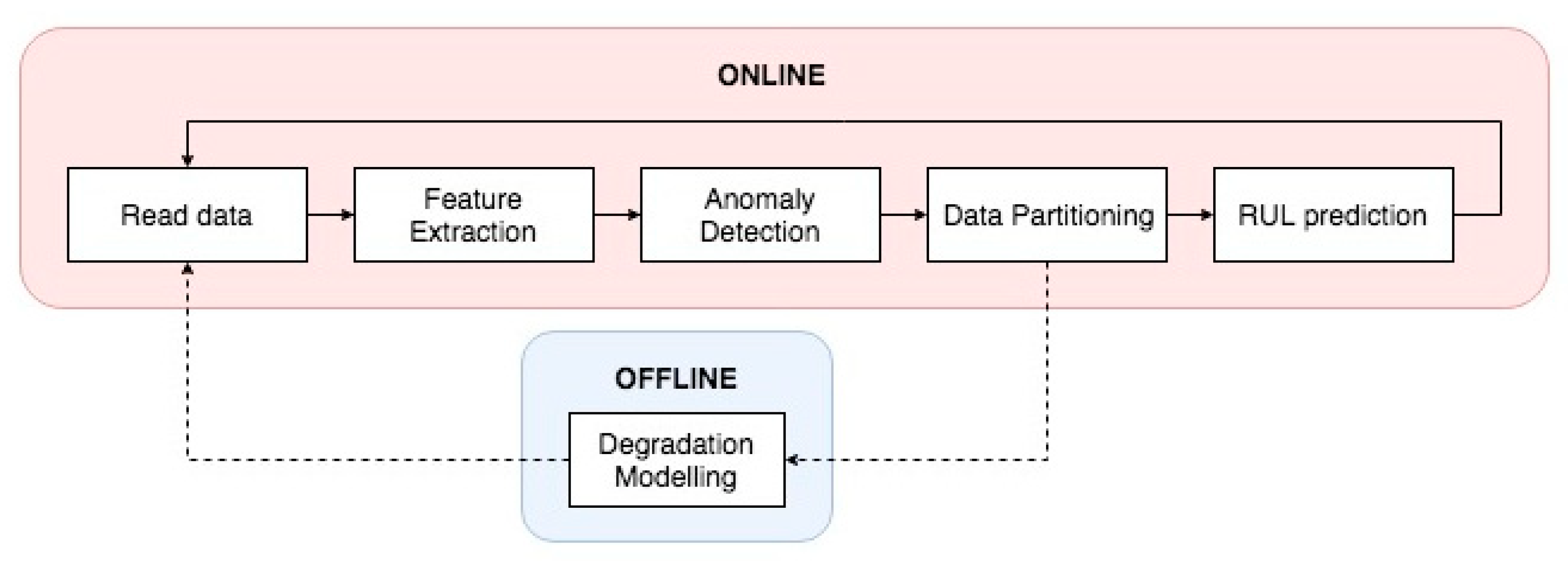
In this paper, we combine feature extraction, HI construction, anomaly detection, HS division, and RUL prediction in a unique methodology, which is unsupervised and suitable for online and real-time implementations of PHM. The aim is to provide a framework that is similar to those applied for batch processes, in which: relevant features are extracted online as data are collected; a monotonic HI is built during the algorithm’s execution; and, the information collected during the anomaly detection and data partitioning algorithms are used for both the degradation modelling and RUL prediction. As shown in Figure 1, the proposed methodology comprises two main blocks: in the first block, which is completely online, anomaly detection and ADP algorithms are combined in order to detect changes in the data structure and form data clouds corresponding to different HS of the degradation process. In the second step, conducted offline, the degradation model for the identified failure is built and a failure threshold (FT) is set. Finally, the so-built degradation model is updated online, as a certain HS is reached for the real-time RUL estimation.

The novel aspect of the proposed methodology is the use of the ADP algorithm for HS division, which makes the procedure unsupervised and implementable “from scratch”. Indeed, in the literature, there exist some examples of online and/or real-time applications of PHM [19,20,21]. However, in such cases, a priori offline analysis is always conducted, not only for the FT identification, but also for diagnostics. In contrast, the proposed methodology does not rely on pre-built classification models. Similar data are automatically grouped in the same clusters and, when an anomaly is detected, the methodology is able to decide whether the following data can form another cluster. The creation of a new cluster certainly requires human intervention to understand what the new cluster corresponds to. However, since all similar data are grouped into the same cluster, the knowledge of what has happened at a specific moment (that is, which condition the observation corresponds to), allows for the automatic labelling of all observations belonging to the same cluster, facilitating a subsequent offline, supervised, and more accurate analysis.

For a clear comprehension of the proposed methodology, the algorithms chosen for anomaly detection, data partitioning, and degradation modelling are described in the first part of the paper. Subsequently, the methodology is applied to a critical component of an automatic machinery operating in a real industrial context. The component under analysis is made of four suction cups, which rotate and push the product forward. When two suction cups become detached, then the component is considered not to perform its function properly, i.e., it is considered to have failed. Suction pressure has been identified by experts as the best indicator for recognizing whether one or more suction cups became detached. The following assumptions have been made: (1) one only sensor is used for signal collection, (2) at the beginning, no prior knowledge is available regarding the current condition of the monitored system, and (3) no historical data is used for training models.

The remainder of this paper is organized, as follows. Section 2 is dedicated to the mathematical formulations of the algorithms adopted for anomaly detection, HS division, and degradation modelling. These algorithms are named autonomous anomaly detection (AAD) and autonomous data partitioning (ADP), which were in proposed by Angelov in [22,23], and are described in Section 2.1 and Section 2.2, respectively, and state space models (SSMs), which are described in Section 2.3. In Section 3, the proposed methodology is introduced, explaining how the described methods can be integrated and applied to a real case. In Section 4, the case study for validating the proposed methodology is presented. Finally, Section 5 is dedicated to the discussion of the main issues that emerged during the application and the future directions of the research.

2. Methods

2.1. Anomaly Detection Based on Recursive Density Estimation (RDE)

RDE is based on the data density, computed recursively as new data become available, used to identify in real time if new data samples differ from previous ones. Data density can be defined as the inverse of the sum of the total distances between all of the data points. It is a measure of the closeness on the $\mathrm{n}$-dimensional feature space of a data sample to all previous data samples at a given time instant. The global data density of the sample ${\mathrm{x}}_{\mathrm{K}}$ available at current time instant $\mathrm{K}$ can be defined as a Cauchy-type function, that for the Euclidean distance type can be expressed, as follows:

$$\mathrm{D}\left({\mathrm{x}}_{\mathrm{k}}\right)=\frac{1}{1+\frac{1}{\mathrm{K}}{{\displaystyle \sum }}_{\mathrm{i}=1}^{\mathrm{K}}\Vert {\mathrm{x}}_{\mathrm{K}}-{\mathrm{x}}_{\mathrm{i}}{\Vert }^2}$$

(1)

This kind of representation allows for an easier recursive calculation, whose formulation can be exactly derived (not in an approximate way) from Equation (1):

$$\mathrm{D}\left({\mathrm{x}}_{\mathrm{k}}\right)=\frac{1}{1+\Vert {\mathrm{x}}_{\mathrm{K}}-{\mathsf{\mu }}_{\mathrm{k}}{\Vert }^2+{\mathsf{\Sigma }}_{\mathrm{k}}-\Vert {\mathsf{\mu }}_{\mathrm{k}}{\Vert }^2}$$

(2)

where ${\mathsf{\mu }}_{\mathrm{k}}$ and ${\mathsf{\Sigma }}_{\mathrm{k}}$ represent the global mean and the scalar product of data sample ${\mathrm{x}}_{\mathrm{K}}$, respectively, at time instant $\mathrm{k}$, which can be calculated recursively, as follows:

$${\mathsf{\mu }}_{\mathrm{K}}=\frac{\mathrm{K}-1}{\mathrm{K}}{\mathsf{\mu }}_{\mathrm{K}-1}+\frac{1}{\mathrm{K}}{\mathrm{x}}_{\mathrm{K}},{\mathsf{\mu }}_1={\mathrm{x}}_1$$

(3)

$${\mathrm{\Sigma }}_{\mathrm{K}}=\frac{\mathrm{K}-1}{\mathrm{K}}{\mathrm{X}}_{\mathrm{K}-1}+\frac{1}{\mathrm{K}}\Vert {\mathrm{x}}_{\mathrm{K}}{\Vert }^2,{\mathrm{\Sigma }}_1=\Vert {\mathrm{x}}_1{\Vert }^2$$

(4)

The terms $\left(\mathrm{k}-1\right)/\mathrm{k}$ and $1/\mathrm{k}$, which are updated at each iteration, can be seen as weight coefficients of the past and current data samples, respectively. This recursive form allows for the storage in memory of only the meta-parameters ${\mathsf{\mu }}_{\mathrm{k}}$ and ${\mathsf{\Sigma }}_{\mathrm{k}}$, making RDE suitable for online applications. Once the data density has been computed at time instant $\mathrm{K}$ by Equation (2), anomalous data can be detected considering the mean data density $\overline{\mathrm{D}}\left({\mathrm{x}}_{\mathrm{k}}\right)$ and the variance of the data density ${\mathsf{\sigma }}_{\mathrm{k}}^2$, whose static formulation is expressed by Equations (5) and (6), and with the recursive calculation of Equations (7) and (8).

$$\overline{\mathrm{D}}\left({\mathrm{x}}_{\mathrm{k}}\right)=\frac{1}{\mathrm{k}}{\displaystyle \sum }_{\mathrm{i}=1}^{\mathrm{k}}\mathrm{D}\left({\mathrm{x}}_{\mathrm{k}}\right)$$

(5)

$${\mathsf{\sigma }}_{\mathrm{k}}^2=\Vert {\overline{\mathrm{D}}}_{\mathrm{K}}-{\mathrm{D}}_{\mathrm{K}}{\Vert }^2$$

(6)

$${\overline{\mathrm{D}}}_{\mathrm{K}}=\frac{\mathrm{K}-1}{\mathrm{K}}{\overline{\mathrm{D}}}_{\mathrm{K}-1}+\frac{1}{\mathrm{K}}{\mathrm{D}}_{\mathrm{K}},{\overline{\mathrm{D}}}_1={\mathrm{D}}_1$$

(7)

$${\mathsf{\sigma }}_{\mathrm{k}}^2=\frac{\mathrm{K}-1}{\mathrm{K}}{\mathsf{\sigma }}_{\mathrm{k}-1}^2+\frac{1}{\mathrm{K}}{\left({\mathrm{D}}_{\mathrm{k}}-{\overline{\mathrm{D}}}_{\mathrm{K}}\right)}^2,{\mathsf{\sigma }}_1^2=1$$

(8)

In particular, while using Equations (7) and (8), anomalies can be detected by resorting to statistical rules or thresholds. For example, in [24], anomalies are detected based on the following condition

$$\mathrm{I}\mathrm{F}{\mathrm{D}}_{\mathrm{K}}<{\overline{\mathrm{D}}}_{\mathrm{K}}-{\mathrm{\sigma }}_{\mathrm{k}}^2\mathrm{T}\mathrm{H}\mathrm{E}\mathrm{N}{\mathrm{x}}_{\mathrm{k}}\mathrm{i}\mathrm{s}\mathrm{a}\mathrm{n}\mathrm{o}\mathrm{u}\mathrm{t}\mathrm{l}\mathrm{i}\mathrm{e}\mathrm{r}$$

(9)

RDE can be successfully applied to fault detection in industrial plants due to its fast responsiveness, computational efficiency, and low memory usage. However, in real applications, where large amounts of data are continuously collected in online mode, it also presents some drawbacks. In particular, when K grows indefinitely, the term $1/\mathrm{K}$ becomes irrelevant with respect to past data, thus reducing the potential informative content of the current data sample and making the RDE algorithm less sensitive to changes in the data structure.

To solve these issues, the RDE with forgetting algorithm was introduced and applied to fault detection [25]. In this formulation, the forgetting factor $\mathsf{\alpha }$ replaces the term $\left(\mathrm{K}-1\right)/\mathrm{K}$, and its complement to 1, $1-\mathsf{\alpha }$ (learning factor), replaces the term $1/\mathrm{K}$, thus enabling static weights over time. It has been demonstrated that RDE with forgetting is suitable for applications where abrupt changes need to be detected.

2.2. Autonomous Data Partitioning Based on Local Data Density

Within the EDA framework, a completely data-driven, unsupervised, and non-parametric clustering method was developed, named autonomous data partitioning (ADP) [22]. The nonparametric measure involved in the algorithm is the local density, whose static and recursive mathematical formulations are expressed in Equations (10) and (11), respectively. The local density identifies the main local mode of the data distribution and is derived empirically from all observed data samples. Different types of distance metrics can be used, e.g., Euclidean distance, Mahalanobis distance, and cosine similarity. Here, formulations that consider Euclidean distance are presented.

$${\mathrm{D}}_{\mathrm{K}}\left({\mathrm{x}}_{\mathrm{k}}\right)=\frac{{{\displaystyle \sum }}_{\mathrm{j}=1}^{\mathrm{K}}{{\displaystyle \sum }}_{\mathrm{l}=1}^{\mathrm{K}}{\mathrm{d}}^2\left({\mathrm{x}}_{\mathrm{j}},{\mathrm{x}}_{\mathrm{l}}\right)}{2\mathrm{K}{{\displaystyle \sum }}_{\mathrm{l}=1}^{\mathrm{K}}{\mathrm{d}}^2\left({\mathrm{x}}_{\mathrm{j}},{\mathrm{x}}_{\mathrm{l}}\right)}$$

(10)

$${\mathrm{D}}_{\mathrm{K}}\left({\mathrm{x}}_{\mathrm{k}}\right)=\frac{1}{1+\frac{\Vert {\mathrm{x}}_{\mathrm{K}}-{\mathsf{\mu }}_{\mathrm{k}}{\Vert }^2}{{\mathrm{X}}_{\mathrm{K}}-\Vert {\mathsf{\mu }}_{\mathrm{k}}{\Vert }^2}}$$

(11)

where ${\mathsf{\mu }}_{\mathrm{k}}$ and ${\mathrm{X}}_{\mathrm{K}}$ can be recursively updated by Equations (3) and (4).

The ADP algorithm, in its evolving form, is able to start “from scratch”, i.e., with a single sample. The first step is the initialization of the global meta-parameters as the first data sample, $\mathrm{K}\leftarrow 1$, is available:

$$\mathrm{NC}\leftarrow 1;{\mathsf{\mu }}_{\mathrm{K}}\leftarrow {\mathrm{x}}_1;{\mathrm{X}}_{\mathrm{K}}\leftarrow \Vert {\mathrm{x}}_1{\Vert }^2$$

where $\mathrm{NC}$ is the number of data clouds. The meta-parameters of the first data cloud are initialized, as follows:

$${\mathrm{C}}_1\leftarrow \left\{{\mathrm{x}}_1\right\};{\mathrm{c}}_{\mathrm{K},1}\leftarrow {\mathrm{x}}_1;{\mathrm{S}}_{\mathrm{K},1}\leftarrow 1$$

where ${\mathrm{c}}_{\mathrm{K},1}$ is the prototype (center) of the data cloud 1 at time stamp $\mathrm{K}$ and ${\mathrm{S}}_{\mathrm{K},1}$ is the number of data samples that belong to the cloud 1 at the time stamp $\mathrm{K}$.

For each newly arriving data sample $\left(\mathrm{K}\leftarrow \mathrm{K}+1\right)$, the global meta-parameters ${\mathsf{\mu }}_{\mathrm{K}}$ and ${\mathrm{X}}_{\mathrm{K}}$ are updated through Equations (3) and (4). Subsequently, the data densities at the current point ${\mathrm{x}}_{\mathrm{K}}$ and at the cloud centers ${\mathrm{c}}_{\mathrm{K},\mathrm{i}}\left(\mathrm{i}=1,2,\dots ,\mathrm{NC}\right)$ are computed using Equation (11). The following condition is checked to decide whether ${\mathrm{x}}_{\mathrm{K}}$ is able to become a new prototype and form a data cloud around itself:

$$\begin{gathered} \mathrm{I}\mathrm{F}{\mathrm{D}}_{\mathrm{K}}\left({\mathrm{x}}_{\mathrm{K}}\right)>\underset{\left(\mathrm{i}=1,2,\dots ,\mathrm{N}\mathrm{C}\right)}{\max }\left({\mathrm{D}}_{\mathrm{K}}\left({\mathrm{c}}_{\mathrm{K}-1,\mathrm{i}}\right)\right)\mathrm{O}\mathrm{R} \\ {\mathrm{D}}_{\mathrm{K}}\left({\mathrm{x}}_{\mathrm{K}}\right)<\underset{\left(\mathrm{i}=1,2,\dots ,\mathrm{N}\mathrm{C}\right)}{\min }\left({\mathrm{D}}_{\mathrm{K}}\left({\mathrm{c}}_{\mathrm{K}-1,\mathrm{i}}\right)\right)\mathrm{T}\mathrm{H}\mathrm{E}\mathrm{N}\left({\mathrm{x}}_{\mathrm{K}}\mathrm{i}\mathrm{s}\mathrm{a}\mathrm{n}\mathrm{e}\mathrm{w}\mathrm{p}\mathrm{r}\mathrm{o}\mathrm{t}\mathrm{o}\mathrm{t}\mathrm{y}\mathrm{p}\mathrm{e}\right) \end{gathered}$$

(12)

If the density at the current point is greater/lower than the density at any of the existing data clouds, that is, if the condition of Equation (12) is satisfied, then a new data cloud is added and ${\mathrm{x}}_{\mathrm{K}}$ becomes the prototype of the new cloud:

$$\mathrm{NC}\leftarrow \mathrm{NC}+1;{\mathrm{C}}_{\mathrm{NC}}\leftarrow \left\{{\mathrm{x}}_{\mathrm{K}}\right\};{\mathrm{c}}_{\mathrm{K},\mathrm{NC}}\leftarrow {\mathrm{x}}_{\mathrm{K}};{\mathrm{S}}_{\mathrm{K},\mathrm{NC}}\leftarrow 1$$

Otherwise, the center of the nearest data cloud ${\mathrm{C}}_{{\mathrm{n}}^{*}}$ to ${\mathrm{x}}_{\mathrm{K}}$ is found, being denoted c_K−1,n^*, and the following condition is checked to see whether ${\mathrm{x}}_{\mathrm{K}}$ is associated with the nearest data cloud ${\mathrm{C}}_{{\mathrm{n}}^{*}}$

$$\mathrm{I}\mathrm{F}\left(\mathrm{d}\left({\mathrm{x}}_{\mathrm{K}},{\mathrm{c}}_{\mathrm{K}-1,{\mathrm{n}}^{*}}\right)<\frac{{\mathsf{\gamma }}_{\mathrm{K}}}{2}\right)\mathrm{T}\mathrm{H}\mathrm{E}\mathrm{N}\left({\mathrm{x}}_{\mathrm{K}}\mathrm{i}\mathrm{s}\mathrm{a}\mathrm{s}\mathrm{s}\mathrm{i}\mathrm{g}\mathrm{n}\mathrm{e}\mathrm{d}\mathrm{t}\mathrm{o}{\mathrm{C}}_{{\mathrm{n}}^{*}}\right)$$

(13)

where ${\mathsf{\gamma }}_{\mathrm{K}}$ is approximately equal to the average distance between all the data samples $\sqrt{{\overline{\mathrm{d}}}_{\mathrm{K}}}$, and it can be computed, as follows: ${\mathsf{\gamma }}_{\mathrm{K}}\approx \sqrt{{\overline{\mathrm{d}}}_{\mathrm{K}}}=\sqrt{2\left({\mathrm{X}}_{\mathrm{K}}-\Vert {\mathsf{\mu }}_{\mathrm{K}}{\Vert }^2\right)}$.

If the distance between the current data point and the center of the nearest cloud is lower than the average distance between all data samples, i.e., if the condition of Equation (13) is satisfied, then ${\mathrm{x}}_{\mathrm{K}}$ is assigned to the nearest data cloud ${\mathrm{C}}_{{\mathrm{n}}^{*}}$, whose meta-parameters are updated, as follows:

$${\mathrm{S}}_{\mathrm{K},{\mathrm{n}}^{*}}\leftarrow {\mathrm{S}}_{\mathrm{K}-1,{\mathrm{n}}^{*}}+1$$

(14)

$${\mathrm{c}}_{\mathrm{K},{\mathrm{n}}^{*}}\leftarrow \frac{{\mathrm{S}}_{\mathrm{K}-1,{\mathrm{n}}^{*}}}{{\mathrm{S}}_{\mathrm{K},{\mathrm{n}}^{*}}}{\mathrm{c}}_{\mathrm{K}-1,{\mathrm{n}}^{*}}+\frac{1}{{\mathrm{S}}_{\mathrm{K},{\mathrm{n}}^{*}}}{\mathrm{x}}_{\mathrm{K}}$$

(15)

Otherwise, ${\mathrm{x}}_{\mathrm{K}}$ is added as a new prototype, and a new data cloud is formed.

2.3. Degradation Process Modelling and RUL Prediction

The occurrence of a failure in a component/system is often the result of a degradation process that is hidden in the condition monitoring data. However, parameters collected through condition monitoring often represent undirect degradation indicators, whose relationship with the latent degradation of the system is unknown. State space models (SSMs) are often adopted to deal with this issue [17]. These models describe the stochastic process describing the degrading progression of the occurrence of a failure in a system. An SSM comprises two parts: the state equation and the observation equation. The first reflects the evolution of the failure, which is usually unmeasurable and, thus, called the latent degradation condition. The observation equation reflects the relationship between the latent degradation condition and the indirect degradation indicator. Mathematically, given an unobservable state process ${\left\{{\mathrm{x}}_{\mathrm{t}}\right\}}_{\mathrm{t}\ge 0}$ and an observation series ${\left\{{\mathrm{y}}_{\mathrm{t}}\right\}}_{\mathrm{t}\ge 0}$, the SSM is completely specified by the initial state distribution $\mathsf{\pi }\left({\mathrm{x}}_0\right)$ and the conditional probability density function $\mathsf{\pi }\left({\mathrm{y}}_{\mathrm{t}}|{\mathrm{x}}_{\mathrm{t}}\right)$ for $\mathrm{t}\ge 1$ [26]:

$$\{\begin{array}{c}\mathsf{\pi }\left({\mathrm{y}}_{\mathrm{t}}|{\mathrm{x}}_{0:\mathrm{t}},{\mathrm{y}}_{1:\mathrm{t}-1}\right)=\mathsf{\pi }\left({\mathrm{y}}_{\mathrm{t}}|{\mathrm{x}}_{\mathrm{t}}\right)\\ \mathsf{\pi }\left({\mathrm{x}}_{\mathrm{t}}|{\mathrm{x}}_{0:\mathrm{t}-1},{\mathrm{y}}_{1:\mathrm{t}-1}\right)=\mathsf{\pi }\left({\mathrm{y}}_{\mathrm{t}}|{\mathrm{x}}_{\mathrm{t}-1}\right)\end{array}=\{\begin{array}{c}{\mathrm{y}}_{\mathrm{t}}=\mathrm{f}\left({\mathrm{x}}_{\mathrm{t}}\right)+{\mathrm{v}}_{\mathrm{t}}\\ {\mathrm{x}}_{\mathrm{t}}=\mathrm{g}\left({\mathrm{x}}_{\mathrm{t}-1}\right)+{\mathrm{w}}_{\mathrm{t}}\end{array}$$

(16)

where the first equation of the system represents the observation equation, while the second represents the state equation; ${\mathrm{x}}_{\mathrm{t}}$ is the unobserved state of the system at time $\mathrm{t}$; ${\mathrm{y}}_{\mathrm{t}}$ is the observation at time $\mathrm{t}$; and, ${\mathrm{v}}_{\mathrm{t}}$ and ${\mathrm{w}}_{\mathrm{t}}$ are the process and measurement noises, respectively, which are independent of each other.

Given an SSM describing the latent degradation process of a system, the main task is to make an inference of the unobserved health state and predict the future state based on CM data. Several empirical models may be used to establish the state evolution equation. Among these, dynamic Bayesian methods provide a unified framework for state estimation of the stochastic process [27,28,29]. The choice of the most suitable type of SSM depends on the nature of the system dynamics and noise source. The most commonly adopted are the Kalman filter (KF), for linear dynamics and Gaussian noise; the extended Kalman Filter (EKF), for non-linear dynamics and Gaussian noise; and, particle filtering (PF), when both the dynamic evolution of the degradation and the noise are non-linear.

In addition to the choice of the specific degradation process models, there are other key aspects in RUL prediction. The first regards the definition of a proper HI that can be used to track the fault progression [30]. This can be one of the extracted features, a combination of the extracted features, or a correlation coefficient between vibration signals that corresponds to different component conditions [31]. It is important that the HI be as monotonic as possible, i.e., it should decrease in time as the degradation increases. To this purpose, a dynamic smoothing/filtering technique can be applied to eliminate anomalous peaks and dips in the HI values that could negatively affect the analysis [32]. The second aspect regards the definition of the time to start the prediction (TSP) [33], which is usually subjectively determined or based on statistical methods. Finally, to compute the RUL, the failure threshold (FT) has to be set. Indeed, the RUL is computed as the time difference between the current time and the time at which the HI is expected to reach the pre-fixed failure threshold. The threshold can be set based on expert judgments, similar components, prior knowledge about the component, or a different algorithm. It is important to note that the RUL is a probabilistic quantity and, therefore, confidence values of the prediction must always be determined.

Finally, evaluation metrics for the model assessment and prediction accuracy have to be established. One of the most adopted metrics is the mean square error (MSE), which is defined as the squared prediction error, where the error is the deviation from the desired output, which, in this case, is the real RUL of the system [34].

3. The Proposed Methodology

The proposed methodology is described in this section. The objective is to provide a description of the steps that should be followed to implement, “from scratch”, a procedure that:

• identifies anomalous behaviours that could potentially represent faults;
• builds a training set for the identification of the corresponding degradation model; and,
• triggers the RUL prediction when most appropriate to anticipate the occurrence of the known fault.

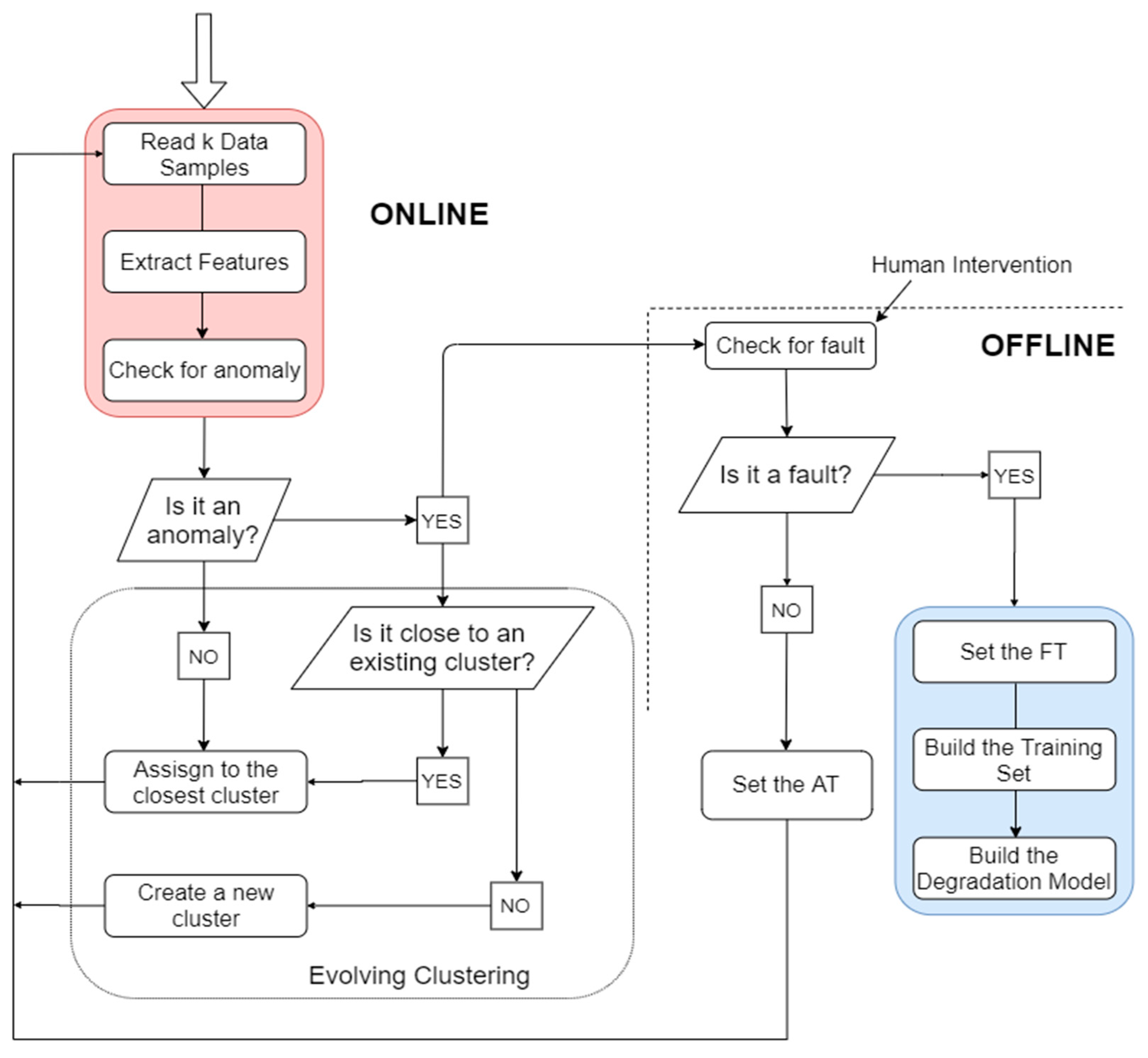
Figure 2 shows the steps included in the methodology, where two main blocks can be distinguished. The online part includes data collection and feature extraction, and aims to detect anomalous behaviours and assign each data sample to a cloud, in such a way that each cloud will correspond to a different HS. As feature vectors are available, for each $\mathrm{k}$ data sample, the online algorithm decides whether a change in the data structure has occurred in real time. When no anomaly is detected, the data sample is automatically assigned to the current data cloud. Otherwise, it could be assigned to an existing data cloud or become the prototype of a new cloud. In addition, in the case in which a data sample is considered to be anomalous, a warning message is generated, which signals to a worker to physically check for the presence of a fault. If no faults are effectively found, then the HI value at which the anomaly was detected can be set as the anomaly threshold (AT), i.e., the time to start the prediction; then, the next k observations are read to begin a new iteration. On the contrary, if a fault is detected, the failure threshold (FT) is identified as the HI value at that time instant; data that are collected until that moment are used as the training set for building the degradation model of the fault.

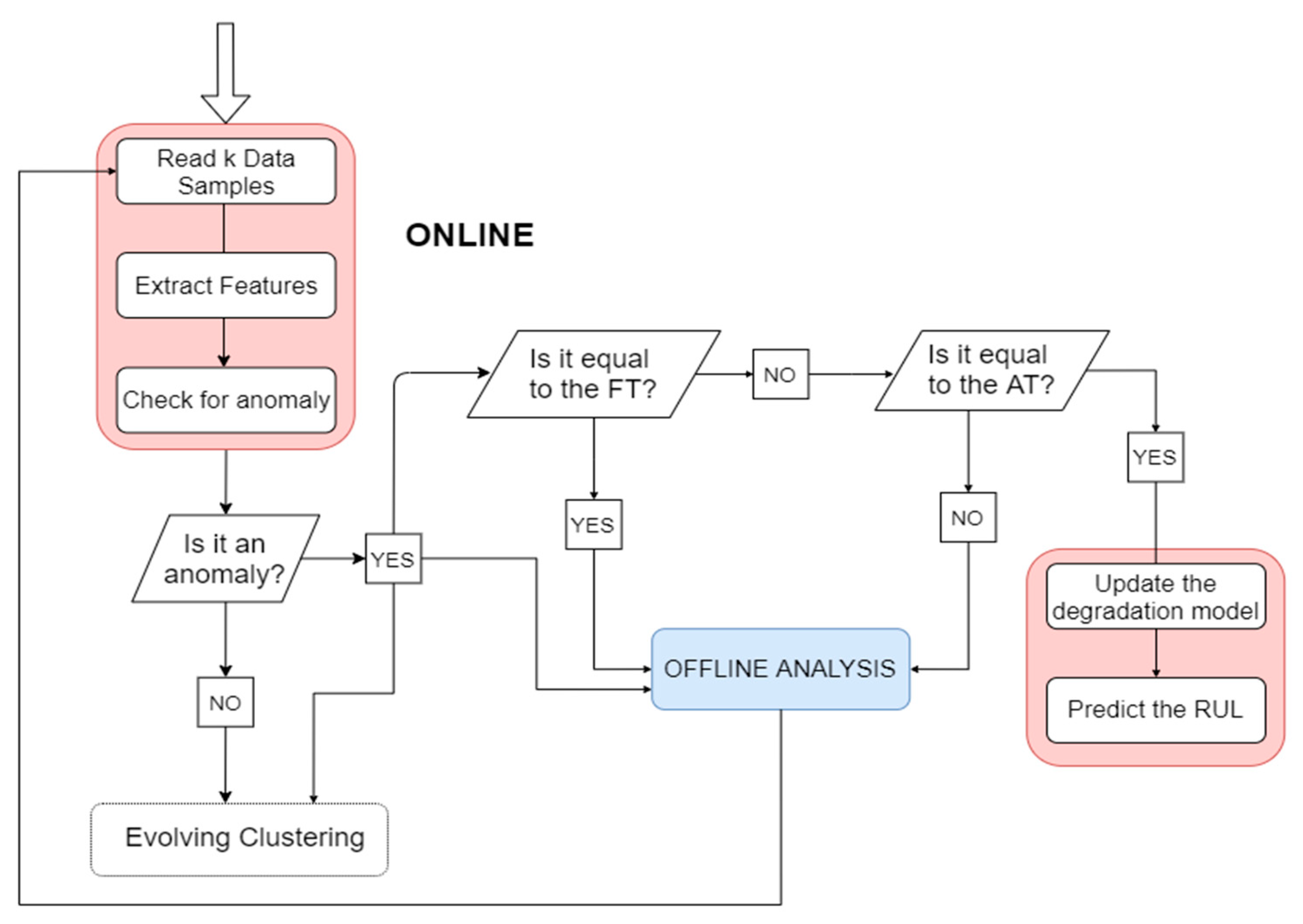
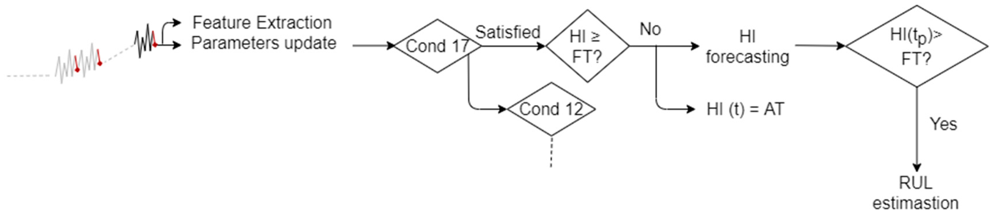
After restoring the correct operating condition of the system, it is possible to use the degradation model that was built during the previous phase. The online part is always activated for detecting anomalies and updating/creating data clouds. However, an additional online part is introduced, which aims to anticipate the occurrence of the fault identified in the previous “training” step. as shown in Figure 3. Indeed, when an anomaly is detected and the FT is reached, then offline analysis is needed to update the degradation model. Otherwise, if the HI value that corresponds to the time instant at which the anomaly is detected is greater than or equal to the AT, and then the future values of the HI begin to be predicted based on the built degradation model and the RUL prediction is triggered. On the contrary, if the current HI value does not exceed the anomaly threshold, but it is nonetheless considered to be anomalous by the online algorithm, then a further offline investigation is needed. In any case, when the RUL prediction is triggered, what we expect is a warning message, showing how long it takes to reach the FT.

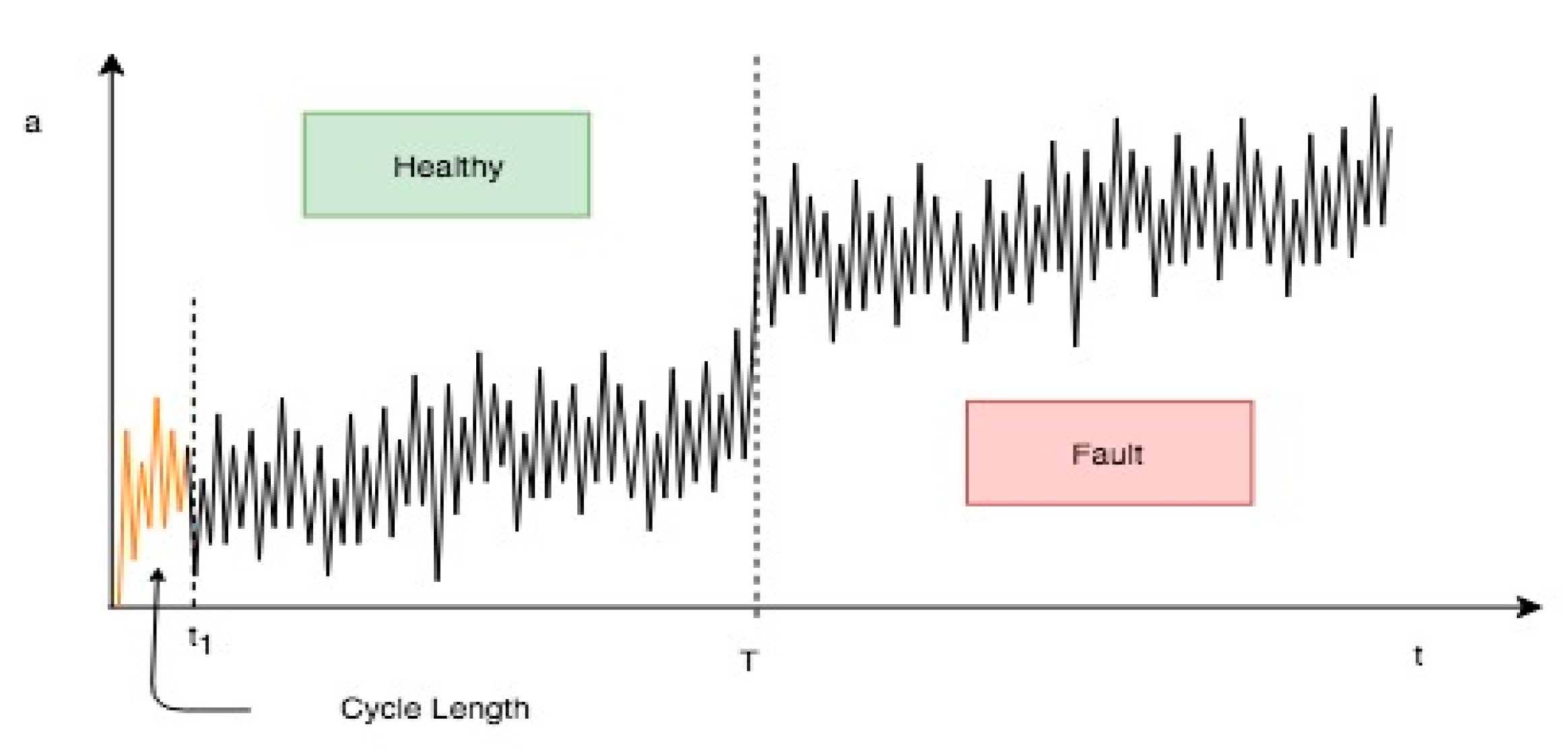
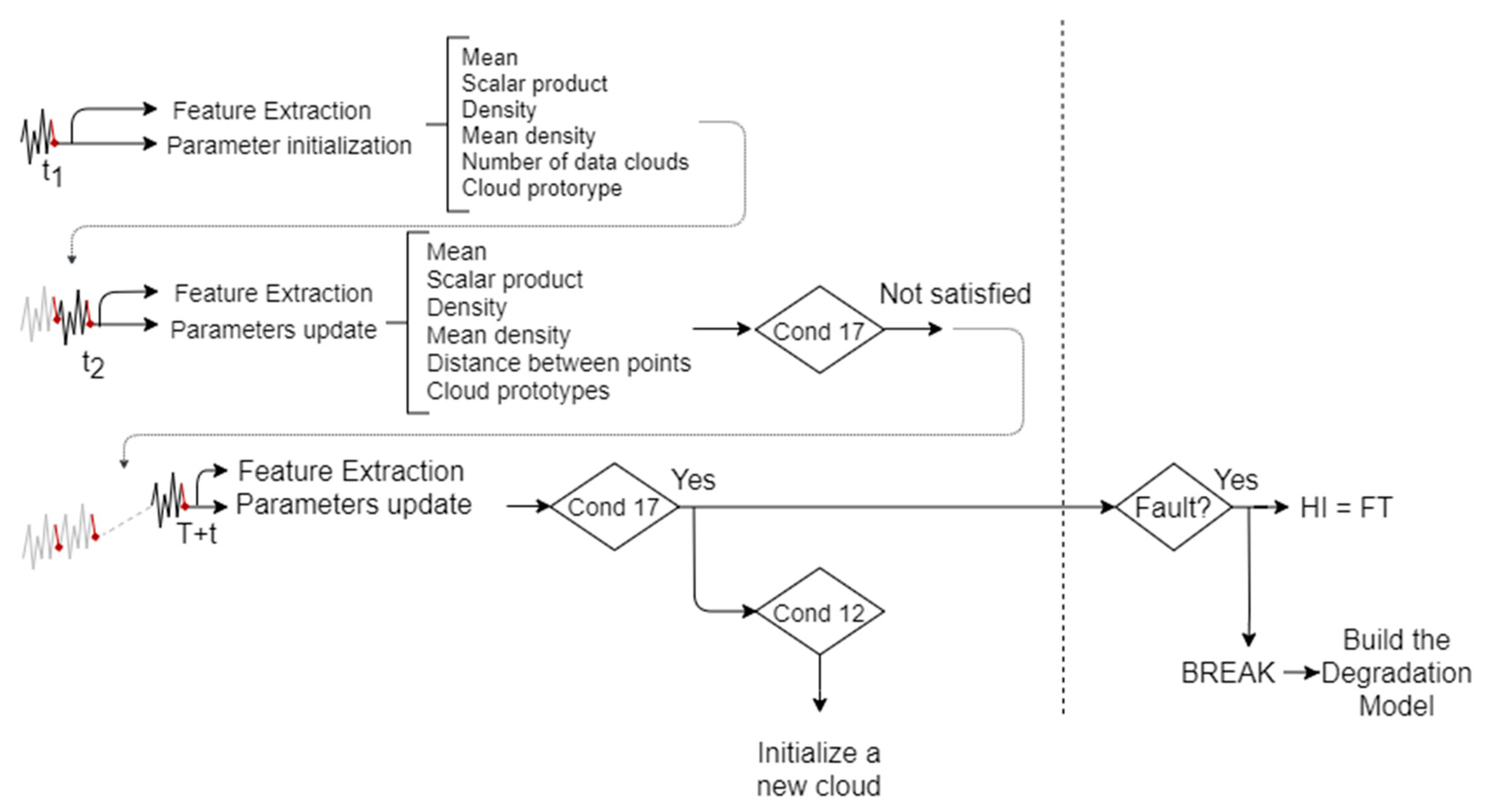
For simplicity, consider the example that is shown in Figure 4, in which vibration data in the healthy and fault conditions are collected at a certain sample frequency $f_s$ through an accelerometer. Suppose that the vibration signature during a certain period of time is in a healthy condition; then, after a time $T$, it enters a fault condition.

The first step is to extract relevant features after $t=f_s·k$, where $k$ is the number of data samples read during the time window considered for one iteration. For example, for rotating machinery, the time window could correspond to the time of one revolution. At the time $t_1$, the feature vector $F\left(t_1\right)$ corresponding to the first signal segment, made up of $k$ data samples, can be memorized, while the $k$ samples can be discarded, as shown in Figure 5.

In addition, both global and local parameters are initialized (see Section 2.1 and Section 2.2). Therefore, the cloud $c1$ is created, which only contains the feature vector $F\left(t_1\right)$. At the second cycle, when the feature vector $F\left(t_2\right)$ corresponding to the second signal segment is available, at the time instant $t_2$, the anomaly detection algorithm can be activated. Actually, because since the current mean density and the global density of the last $n$ data samples are usually compared for establishing whether a data point is an anomaly, the algorithm can be triggered after $n$ feature vectors are collected.

Now, suppose that we are at the $\mathrm{j}(\mathrm{j}>\mathrm{n})$ data point; an anomaly is detected if the mean data density is greater than the density of the last $n$ points [34]:

$$\mathrm{I}\mathrm{F}\mathrm{D}\left(\mathrm{j}\right)<{\mathsf{\mu }}_{\mathrm{D}}\mathrm{j}=\mathrm{j}-\mathrm{n},\dots ,\mathrm{j}\mathrm{T}\mathrm{H}\mathrm{E}\mathrm{N}\mathrm{j}\mathrm{i}\mathrm{s}\mathrm{a}\mathrm{n}\mathrm{a}\mathrm{n}\mathrm{o}\mathrm{m}\mathrm{a}\mathrm{l}\mathrm{y}$$

(17)

where:

$${\mathsf{\mu }}_{\mathrm{D}}=\left(\frac{\mathrm{k}\mathrm{s}-1}{\mathrm{k}\mathrm{s}}{\mathsf{\mu }}_{\mathrm{D}}+\frac{1}{\mathrm{k}\mathrm{s}}\mathrm{D}\left({\mathrm{x}}_{\mathrm{k}}\right)\right)\left(1-{\Delta }_{\mathrm{D}}\right)+\mathrm{D}\left({\mathrm{x}}_{\mathrm{k}}\right){\Delta }_{\mathrm{D}}$$

(18)

$${\Delta }_{\mathrm{D}}=\left|\mathrm{D}\left({\mathrm{x}}_{\mathrm{k}}\right)-\mathrm{D}\left({\mathrm{x}}_{\mathrm{k}-1}\right)\right|$$

(19)

$\mathrm{ks}$ represents the number of data samples that belong to the same condition. It can be seen as a forgetting factor. Indeed, it is incremented by 1 until a new condition is detected. When the system enters the fault condition, then $\mathrm{ks}=0$.

In this case, $F\left(t_2\right)$ belongs to the same condition as $F\left(t_1\right)$: no anomaly is detected, the data point is assigned to the cloud c₁, and its parameters are updated, based on the rules of the ADP algorithm (see Section 2.2). This operation is repeated each $t$, until the condition of Equation (17) is satisfied. When the feature vector $F\left(T+t\right)$ is available, the algorithm recognizes the corresponding data sample as an anomaly and a new cluster $c2$ is created. At this point, the offline analysis can be conducted. Suppose that a real fault exists. Hence, the HI value that corresponds to the data samples that triggered the generation of the new cloud is set as FT; data points of clouds $c1$ and $c2$ are used to build the training set, which is finally used for building the data-driven degradation model corresponding to the identified fault.

Because a fault has occurred, the correct operating condition must be restored. Therefore, the procedure described thus far is applied again to the system in the healthy condition, with the difference that, this time, the local parameters of the identified clouds (e.g., number of clouds, cloud prototypes, cloud mean densities) are given as inputs to the algorithm. In addition, at a certain time, the HI values will be predicted in the future according to both the model built during the offline analysis and the new available data points. The RUL is computed as the difference between the moment at which the HI value is supposed to reach the prefixed failure threshold and the current time. If an anomaly value not exceeding the FT has been detected, then the corresponding HI value can be considered as the time to start RUL prediction (Figure 6).

When an anomaly is detected, but a fault has not actually occurred, then the algorithm must continue. Therefore, it is necessary that the current anomalous condition is considered to be normal to detect eventual other anomalies. To do so, when the status of the system is declared anomalous, the following condition is checked [34]:

$$IFD\left(j\right)>{\mu }_{D}j=j-\mathrm{m},\dots ,jTHENjisnotanymoreananomaly$$

(20)

That is, if the current global density is greater than the mean density for $\mathrm{m}$ data samples, then the status of the system can be declared normal. From this point, the joint anomaly detection and ADP can be triggered again each time that a feature vector is available.

4. Results

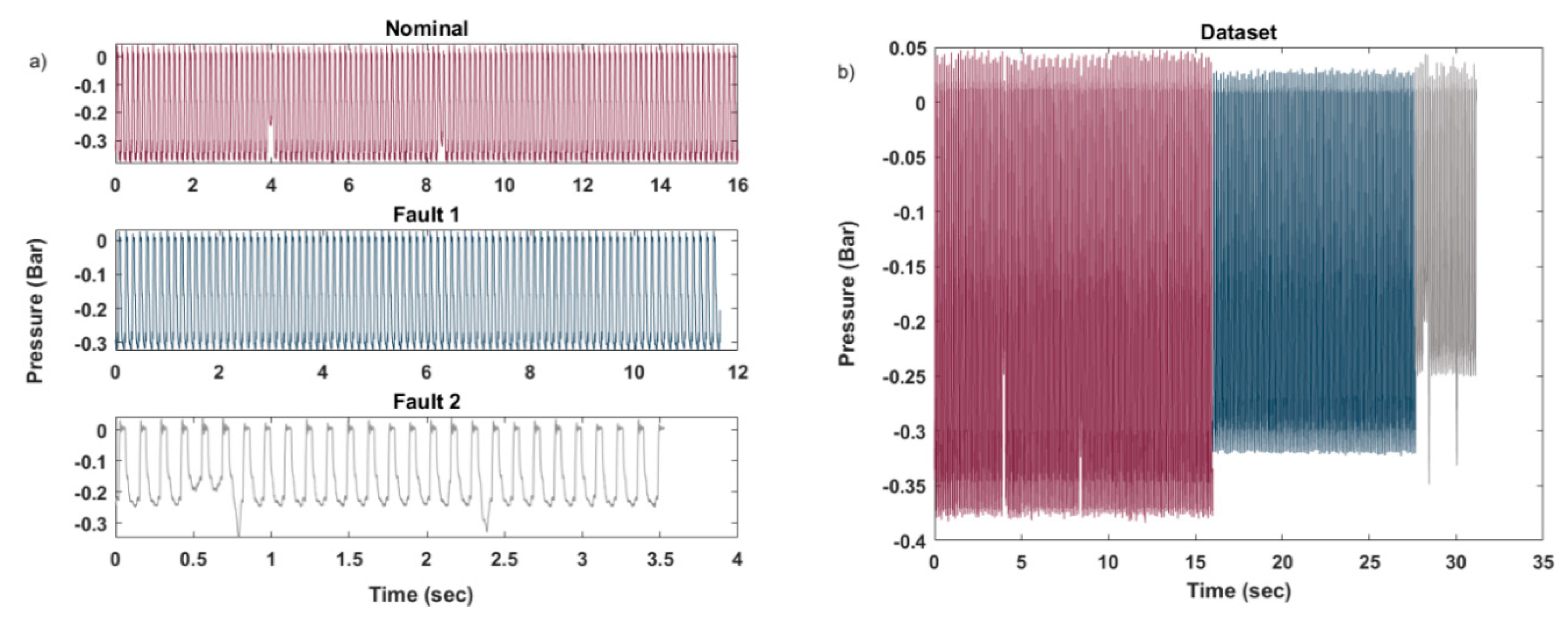
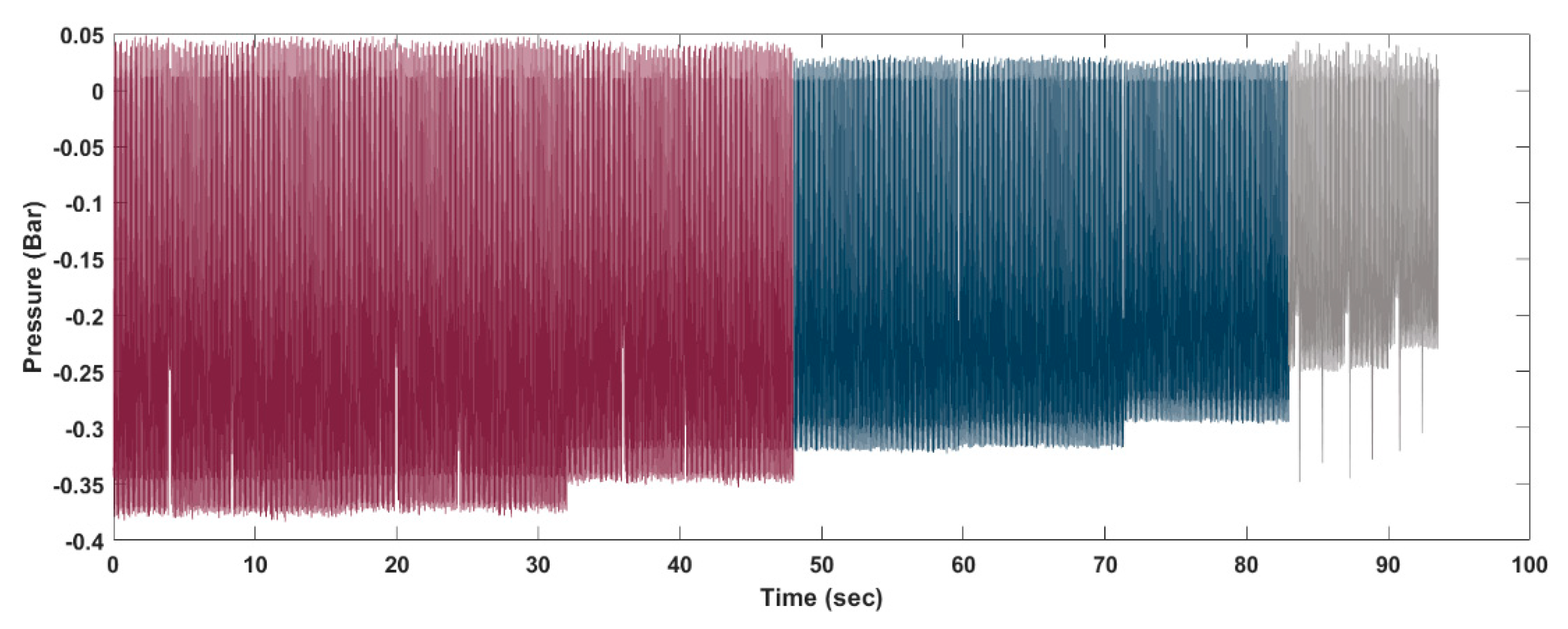
In this section, a case study showing how the proposed innovative procedure can be implemented for predicting the RUL based on streaming data is introduced. The component under analysis is a critical part of an automatic machine, whose malfunctioning strongly affects the quality of the products. The component is made of four suction cups, which rotate and push the product forward. The time length of a cycle is 0.134 s. The main problem that is related to this component is that, at each cycle, the pressure of the suction cups on the product decreases until one or more of the suction cups becomes detached. It has been noted that if one only suction cup becomes detached, then the quality of the resulting product is still acceptable; however, if two suction cups become detached, then the component is not able to perform its function properly. The measure that best describes the correct functioning of the component under analysis is the pressure. Therefore, the pressure (unit: bar) is collected at a sampling frequency of 10 kHz, under three conditions, named Nominal, Fault 1, and Fault 2, where Fault 1 represents the state in which only one suction cup is missing and Fault 2 represents two suction cups missing. The pressure values in the different conditions are shown in Figure 7. Note that the test during which data was collected was not performed for maintenance purposes. Thus, the choice of the sampling frequency was derived from other considerations.

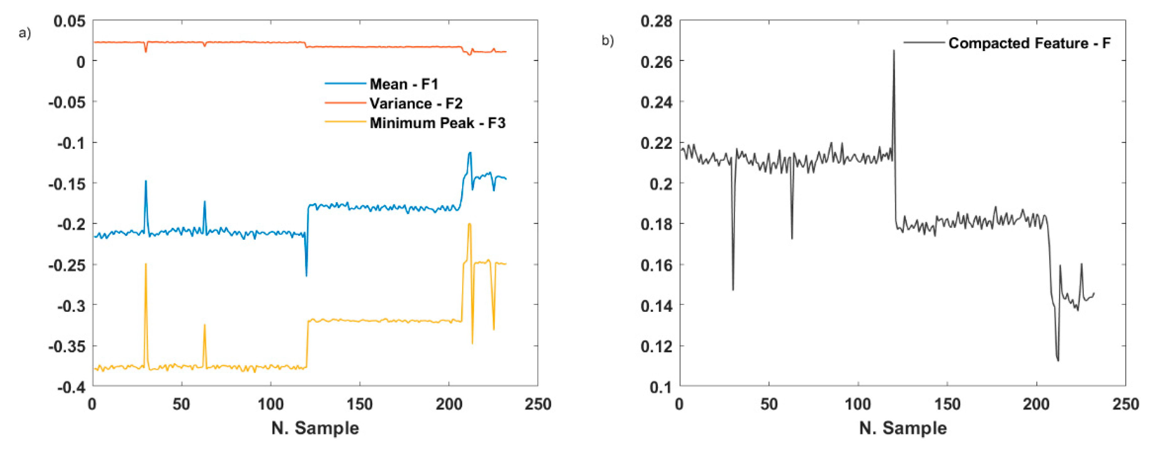
The first step was to identify the segment length for the feature extraction, i.e., the number of data samples, $k$ in the time window $t$, from which features are extracted. Subsequently, a decision regarding which features to extract was made. Time-domain features are the most appropriate in streaming applications. Therefore, a brief analysis was made of the most typical time features and the results showed that the most discriminant features are, in this case, the mean, variance, and minimum peak, as shown in Figure 8a. Subsequently, a synthetic value of the extracted features is computed, as follows:

$$\mathrm{F}=\sqrt{{\mathrm{F}}_1^2+{\mathrm{F}}_2^2+{\mathrm{F}}_3^2}$$

(21)

This value is shown in Figure 8b and it represents the value on which the anomaly detection is based.

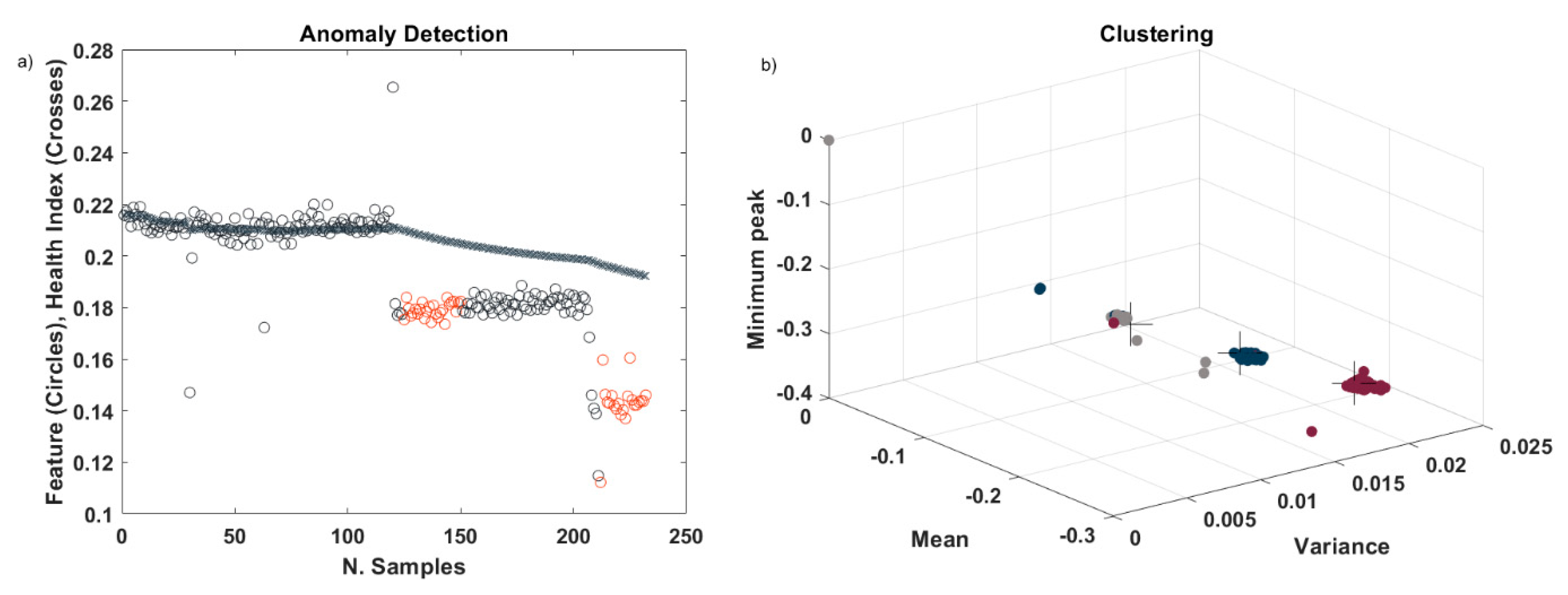
Because the performance of the proposed procedure mostly depends on the ability to detect anomalies, we first validate anomaly detection and ADP algorithms on the described dataset, treating it as a streaming dataset. In this case, two anomalies were detected, as expected. In

Table 1. Performance of the anomaly detection algorithm.

Time (Real) (s)	Detection Time (s)	Latency Time (s)
15.9999	16.7498	0.75
27.6547	28.4079	0.808

, the time instants at which the algorithm recognized the occurrence of a change in the data structure are summarized.

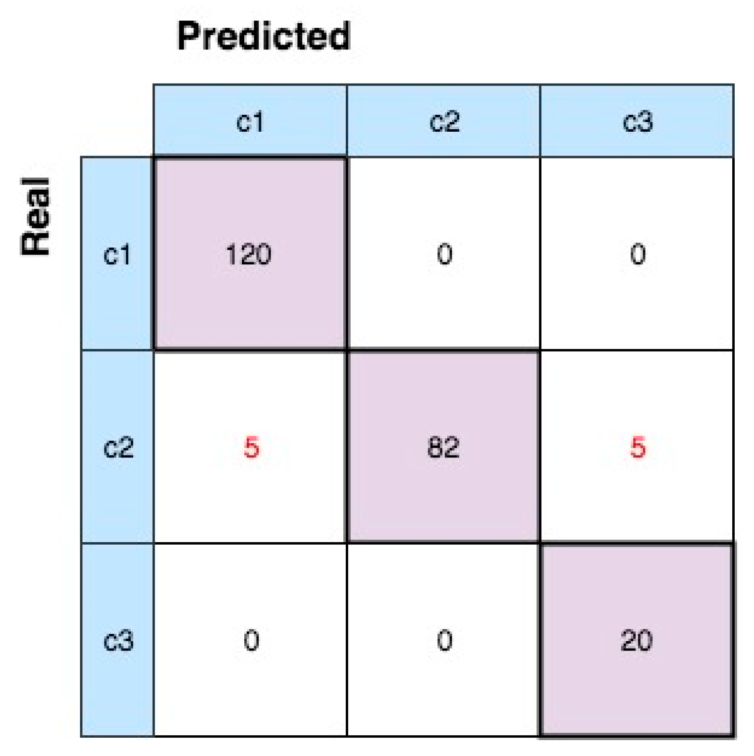
We can conclude the algorithm was able to correctly identify two behavior changes, as shown by the red dots in Figure 9a with latency times of 0.75 and 0.808 s. In addition, as shown in Figure 9b, three clusters were created, which confirms that three different conditions were present in the dataset. Because actual data clusters (labels) are available, the confusion matrix can be used in order to evaluate the performance of clustering (Figure 10). This is a graphic representation that shows the number of observations correctly assigned to a data cloud (true positives) versus the number of misclassifications. The presence of 10 data samples erroneously clustered is due to the latency time for detecting the two anomalous states.

The mean value of data samples is recursively updated at each time stamp during the execution of the anomaly detection algorithm. In this case, this value decreases as time passes and the system degrades, i.e., it is a monotonic function. Therefore, the mean value computed at each time stamp is stored and used as the HI for building the degradation model. In this way, online smoothing techniques for making the synthetic feature value monotonic are avoided and the algorithm is computationally faster and more efficient. The black crosses in Figure 9a show the evolution of HI values with time.

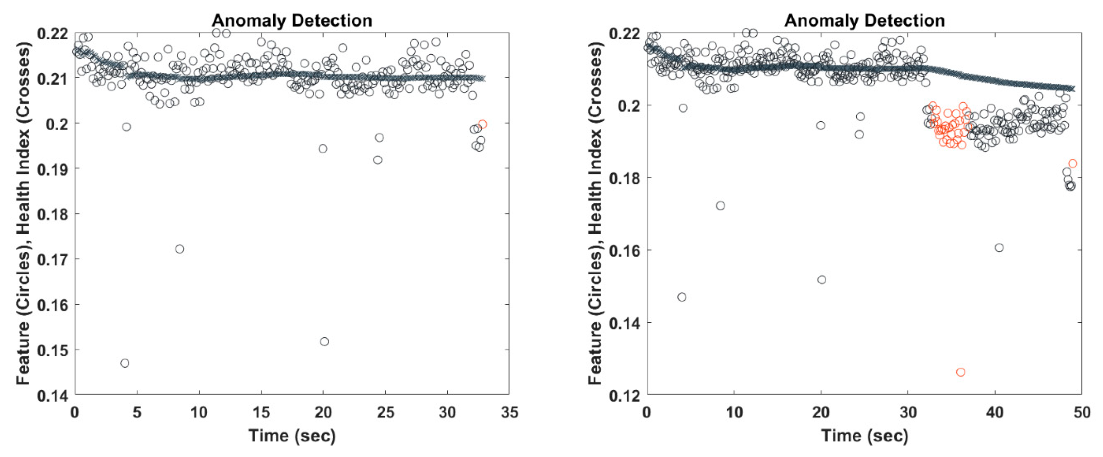
A second dataset of the same system was used for testing the complete procedure and computing the RUL of the system in a completely online way. This time, pressure values in each condition were collected over a longer time period. In particular, as shown in Figure 11, a complete degradation process from the nominal condition to Fault 2 (that corresponds to the condition in which the component has to be fixed) was simulated. In this way, it was also possible to evaluate the sensitivity of the anomaly detection algorithm to slight variations of the monitored parameter, and identify the best time to start updating the degradation model and, thus, the RUL prediction. Indeed, based on the synthetic feature $\mathrm{F}$, computed at each time stamp $\mathrm{k}$, the first anomaly was detected after 32.8299 s (Figure 12a). However, the system entered the condition Fault 1 after $\mathrm{t}=47.9997$. This means that the detected anomalous data sample does not actually correspond to a real fault, but can correspond to an indication that something is happening. Indeed, based on the way the degradation dataset was built, we know that, at that time, a significative reduction of the pressure value occurred.

Therefore, this can be named the anomaly threshold (AT), and it is considered to be the time at which to start updating the model degradation and RUL prediction for future implementations. When the second anomaly is detected at $\mathrm{t}=48.9099$ (Figure 12), a real fault has actually occurred. Subsequently, the HI value at the current time stamp represents the FT.

At this point, the offline analysis can be conducted. Here, an SSM is implemented using the function for the state space model estimation, ssest, as provided by the predictive maintenance toolbox in MATLAB, which initializes the parameter estimates while using a non-iterative subspace approach and refines the parameter values using the prediction error minimization approach.

The obtained model fits the estimation data at 95.51% with the mean square error (MSE) equal to 4.935 × 10⁻⁸. For the implementation to streaming data, the model should be updated as new data are available. For the model updating, three decisions have to be made, which strongly affect the prediction results.

The first decision relates to the time interval, TI, or number of time stamps, between two model updates, when considering that, the higher the value of TI, the lower the prediction ability. The second decision regards the number of HI values that the model has to predict, named HI_f. A large number of predicted values lowers the performance of the prediction algorithm. However, a small number of predicted values may lead to estimating the achievement of the failure threshold too late to allow for a proper scheduling of the intervention. Finally, the number of past data samples used for updating the model has to be correctly defined, named the segment length (SL). A small number is preferred, so that the updates depend on the most recent data samples. However, in this case, even a small peak or drop in the HI trend could affect the prediction performance. On the contrary, if the model updating algorithm takes a high number of previous HI values into account, it takes long time to recognize a fast degradation behavior. Now, suppose that the nominal condition is restored. The online procedure is implemented again. The model updating and RUL prediction are triggered as the system achieves the AT determined in the previous step. Here, different parameter settings are tested, and the results are shown in

Table 2. Comparison of the state space model (SSM) performance with different input parameter sets.

SL	HIf	TI	Detection Time (s)	Predicted RUL (s)	Real RUL (s)	Run Time (s)
100	10	10	48.9099	0.1341	0	45.445
100	20	20	46.2299	2.1441	2.68	23.882
50	10	20	47.5699	0.1341	0	24.304
30	20	20	48.9099	0.1341	0	22.585

.

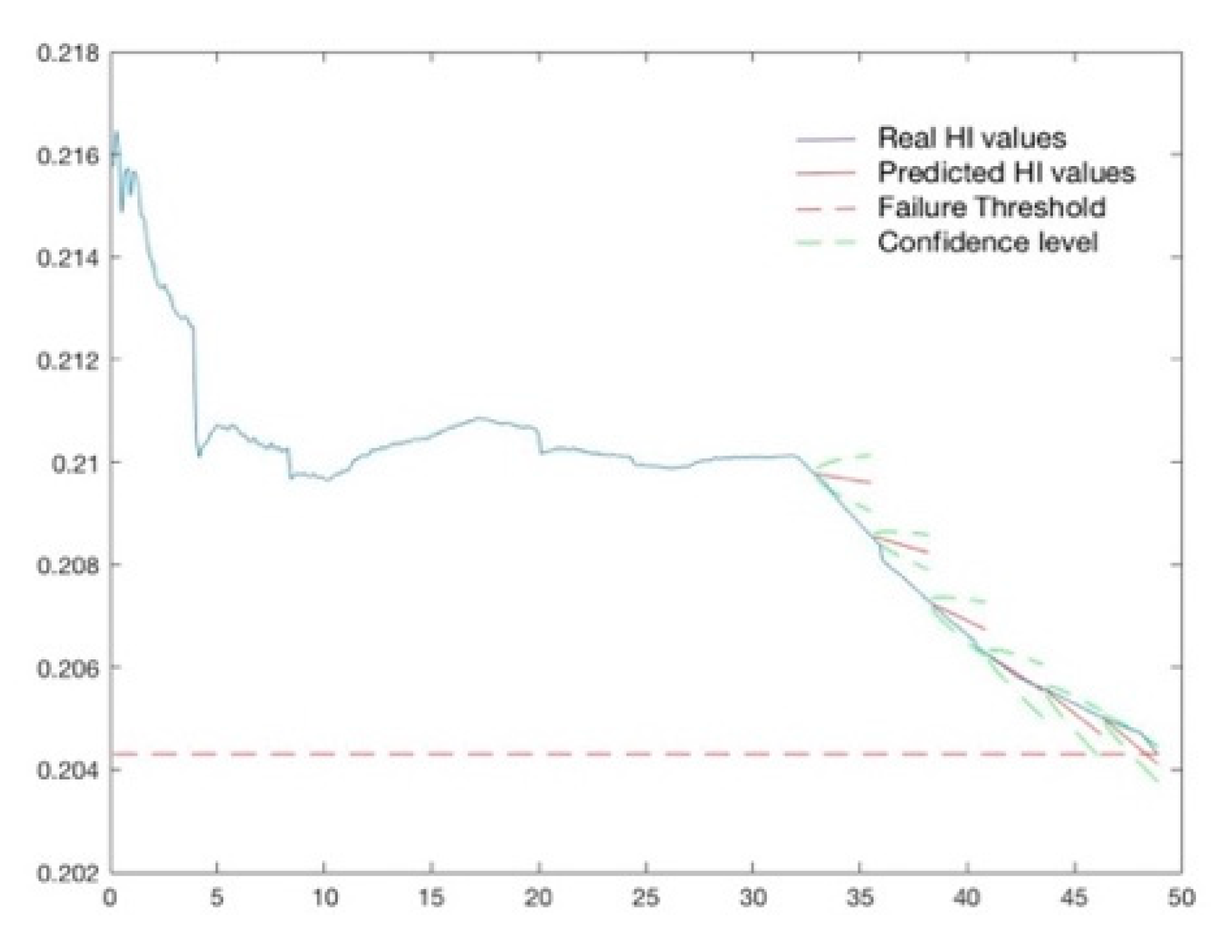
The best performance, in terms of prediction accuracy and RUL, is provided by the parameter set in the second row of Table 2. Figure 13 shows the results, where the blue line shows the HI values over time. The dashed red line represents the FT and the red segments represent the predicted HI values every time the degradation model is updated. In this case, the algorithm starts to predict the HI values and the RUL after 32.8299 s, the time at which the AT is reached. Hence, each $\mathrm{t}=20$ s, the model is updated and 20 HI values are predicted. At the time instant $\mathrm{t}=46.2299$, the model predicts that the HI value will reach the FT after 2.1441 s. This corresponds to a pessimistic prediction, since the fault will actually occur after 2.68 s, thus losing 0.5359 s of the residual life. In the other three cases, the model predicts Fault 2 will occur after 0.1341 s, while actually the FT at the detection time has been already reached (RUL = 0).

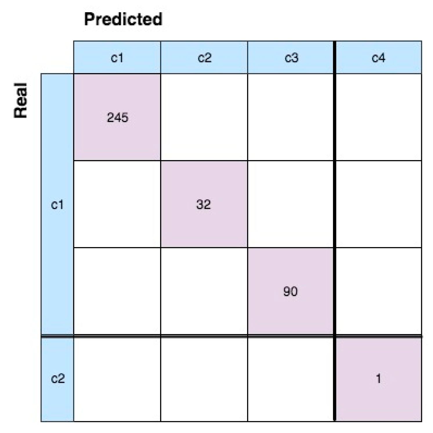
In Figure 14, the confusion matrix of the ADP algorithm that is applied to the new dataset is illustrated. We know that two different conditions are included in the generated dataset until the FT is reached. However, the ADP forms four different data clouds, which may represent four different HS of the degradation process. Data cloud 2 is created when the AT is reached. This means that the first data cloud can be labelled “normal” and the HI values in cloud 2 can be used for a better determination of the AT. In addition, further offline analysis can highlight that there is another “normal” HS before the fault condition. Subsequently, the computational efficiency of the algorithm can be improved by moving the time to start the prediction forward.

Note that Angelov et al. provided the original code for anomaly detection in [23], while the download of the code of the ADP algorithm is available at the website in [22]. Here, an integration of the two algorithms was performed, and the online time feature extraction was added.

5. Discussion and Conclusions

In this paper, we proposed a new PHM methodology for the implementation of fault detection and RUL prediction when there is no prior knowledge regarding the component behavior and only streaming data are available. First, we provided mathematical formulations of the two most promising algorithms for online anomaly detection and data partitioning, which are included in the EDA approach and based on RDE. Subsequently, the main aspects of degradation modelling and RUL prediction are highlighted. These three parts were all included in the proposed methodology, which can be applied from the first data sample that is read. Finally, the new method was applied to a rotating machine operating in a real industrial context. From this application, several considerations have emerged.

The proposed methodology: (1) recognizes the occurrence of an anomaly in the streaming data collected from the monitored machinery; (2) detects the presence of different HS that are represented by different data clouds; (3) is computationally efficient and able to predict the RUL in real time; and (4) requires little data storage capacity. In addition, if a failure is already known, then it can be represented by an existing cloud, with local parameters being associated with the ADP algorithm, and incremental classification can be included in the methodology.

As demonstrated in this paper, the first applications of the proposed methodology show interesting results. However, there are some aspects that are related to each step that make its implementation in real industrial contexts challenging.

Issues related to the online feature extraction can be summarized as:

• The number $k$ of data samples included in the time window form where features are extracted has to be known a priori. In addition, a fixed $k$ might be unsuitable for non-stationary signals.
• The computation time for feature extraction has not to exceed the time available to collect the next $k$ values.
• Even if time features are suitable for online applications, they may not distinguish different component conditions.

Issues that are related to the online anomaly detection can be summarized as:

• Gradual changes are more difficult to recognize than abrupt change.
• The latency time of the algorithm depends on a parameter defined by the user (see Equation (20)). In particular, the switch from one condition to another should be recognized as soon as possible for reducing misclassification errors during data partitioning; at the same time, if the algorithm is too sensitive to an anomalous value, many false alarms will be generated.

Issues that are related to the HI construction can be summarized as:

• The HI value used in this paper might be a good solution for avoiding the smoothing technique. However, the recursively computed mean value tends to increase/decrease too slowly, which makes it harder to identify the correct FT.

Issue related to RUL prediction can be summarized as:

• Given the dynamic nature of the industrial environment and the possibility of different operating conditions of the component, it would be desirable to have a dynamic FT, computed based on the evolving data structure.
• Given these issues, further research will be dedicated to online feature extraction, anomaly detection algorithm, and the identification of proper HI and FT.