Application of Machine Learning for the Automation of the Quality Control of Noise Filtering Processes in Seismic Data Imaging

Abstract

Seismic imaging is the main technology used for subsurface hydrocarbon prospection. It provides an image of the subsurface using the same principles as ultrasound medical imaging. As for any data acquired through hydrophones (pressure sensors) and/or geophones (velocity/acceleration sensors), the raw seismic data are heavily contaminated with noise and unwanted reflections that need to be removed before further processing. Therefore, the noise attenuation is done at an early stage and often while acquiring the data. Quality control (QC) is mandatory to give confidence in the denoising process and to ensure that a costly data re-acquisition is not needed. QC is done manually by humans and comprises a major portion of the cost of a typical seismic processing project. It is therefore advantageous to automate this process to improve cost and efficiency. Here, we propose a supervised learning approach to build an automatic QC system. The QC system is an attribute-based classifier that is trained to classify three types of filtering (mild = under filtering, noise remaining in the data; optimal = good filtering; harsh = over filtering, the signal is distorted). The attributes are computed from the data and represent geophysical and statistical measures of the quality of the filtering. The system is tested on a full-scale survey (9000 km${}^2$) to QC the results of the swell noise attenuation process in marine seismic data.

1. Introduction

For the oil and gas industry, localizing and characterizing economically worthwhile geological reservoirs is essential. Nevertheless, easy-to-exploit reservoirs are relatively rare, and target exploration techniques are becoming increasingly sophisticated. As a result, the requirements for high-quality seismic images in terms of both the signal-to-noise ratio (SNR) and the regularity and density of sampling are constantly increasing [1]. The seismic dataset is always contaminated by different types of noise and unwanted reflections; therefore, the noise attenuation is an important step in a typical seismic data processing sequence. As with every important step, performing quality control (QC) after each noise attenuation process is essential to ensure that noise has been sufficiently removed while no useful signal has been distorted. The QC process is time-consuming and often requires precious human resources to perform a visual inspection of several seismic products. Improving the efficiency and the turnaround of seismic processing projects can be achieved by automating the QC process. Machine learning techniques such as deep neural networks or support vector machines [2] have been widely used in various domains to automatically predict several patterns from relevant features and hence was used to automate numerous human observation-based assessment processes. Here, we investigate the use of those techniques to automate the quality control process of seismic data.

2. Context and Related Work

2.1. Machine Learning for Quality Control Assessment Process

In the current state of the art, machine learning techniques were used to automate various industrial inspection tasks. ref. [3] showed the potential of convolutional neural networks in automating the quality control process of the Printing Industry using deep neural network soft sensors achieving a classification accuracy of 98.4 %. In medical imaging, assessing manually the quality of magnetic resonance image is time- and cost-intensive. ref. [4] proposed a machine learning-based reference-free magnetic resonance quality assessment framework that is trained on human observation derived labels to assess magnetic resonance image quality immediately after each acquisition. To the best of our knowledge, several research works (e.g., [1,5,6]) tried to use machine learning and specifically deep learning techniques to denoise the eismic data but only [7] aim to automate the quality control of seismic imaging filtering process.

Early work on the use of statistical data mining for QC was reported by Spanos et al. [8], where statistical metrics or attributes computed from the seismic data are used in an unsupervised way to assess the quality of a filtering process. The assessment was binary (i.e., either the filtering is normal or it shows some anomalies and it was based on outlier detection). This methodology was an exploratory step towards the development of a data-driven automated QC platform that takes into account techniques from the fields of statistics and machine learning. The work of the authors in [9] further expands the initial work above and proposes the use of a supervised learning-based approach for training data to build an automatic classifier using a support vector machine (SVM) to predict the type of filtering (mild, optimal, or harsh).

2.2. Feature Transformation and Dimensionality Reduction

Ensemble-based statistical attributes that measure the similarity between the filtered seismic image (output) and the residual image (output-input) are used to assess the quality of the denoising process. In the case of optimal filtering, these attributes will not show any similarity (i.e., correlation) between the output and the difference. This assumption comes from the fact that the signal (i.e., output) has nothing in common with the noise (residual) in the case of ideal filtering. When there is a signal distortion or residual noise, the level of similarity will increase as some noise is also present in the output or a signal is also present in the difference, and this will be picked up by the attributes. Authors in [9] proposed using principal component analysis (PCA) as a feature transformation technique to improve the separability of attributes, and hence, to ease the construction of the decision space. Although PCA decomposition allows the extraction of uncorrelated features, nonlinearity in the relationship between attributes and their high dimensionality are two potential limitations of this method. To overcome this issue, a new method for performing a nonlinear PCA was introduced in [10], which suggested computing principal components in high-dimensional feature space using integral operator kernel functions and was used for pattern recognition. In another context (i.e., feature matching) [11] highlighted the power of kernel (i.e., polynomial) approximation for a more efficient representation of the extracted patches (circular shape window around the key-points of a given image).

However, kernel-based PCAs, as well as linear PCAs, are unable to extract independent components since the data distribution along the attributes is not necessarily Gaussian. Independent component analysis (ICA) is a statistical technique that aims to find a linear projection of the data that maximizes an inter-dependency criterion [12].

2.3. Classification Methods

The work proposed by the authors in [9] uses a support vector machine [2] with a polynomial kernel to predict the quality of the denoising process. Different approaches exist when it comes to using binary support vectors to perform multiclass prediction tasks. The work proposed in [13] described the one-against-all strategy as a set of one SVM per class trained to predict one class from a sample of all the remaining classes; the classification is performed according to the maximum output among all SVMs. In contrast, the one-against-one approach, also known as “pairwise coupling”, “all pairs”, or “round-robin”, consists of building one SVM for each pair of classes. The classification of one testing sample is usually done according to the maximum voting, where each SVM votes for one class. Although SVMs are efficient predictors, especially when it comes to binary classification, other models exist and they are more or less efficient depending on the classification task and the complexity of the training set. Random forest, introduced in [14], is one of them. According to to [14], decision trees are very attractive for their high training speed; however, trees derived from traditional models cannot handle training sets with high complexity. In [14], authors built multiple trees in randomly selected subspaces of the feature space. Unlike SVMs, random forests are able to perform multiclass prediction tasks without using multiple binary classifiers. Authors in [15] observed that the one-against-all random forest strategy achieves better classification performance than common random forest and is more robust to outliers.

Unlike all the classifiers already cited, the neural network architecture is very difficult to tune. Many autonomous deep neural network-based algorithms have been designed (e.g., SGNT [16], NADINE [17], ADL [18]) to manage the prediction of data streams. They aimed to automatically build a neural network architecture by performing growing and pruning operations for hidden layers and nodes, respectively, when it comes to underfitting and overfitting.

3. Methods

To automate quality control of the denoising process [9], ensemble-based (e.g., group of sensors) statistical attributes that measure the level of similarity between the output of the filtering and the residual (the difference between the output and the input) are used. In the case of optimal filtering, the residual consists only of the remaining noise after a filtering operation; therefore, these attributes will not show any similarity between the difference and the output (i.e., correlation). When signal leakage or residual noise is observed, the level of similarity will increase as some noise is also present in the output or some signal is also present in the difference, and this will be picked up by the attributes. The Pearson cross-correlation, Kendell cross-correlation, and mutual information are examples of attributes that capture the correlation between the filtering output and the difference [19]. The cross plots of five different attributes computed from three test lines are shown overlaid for the three types of filtering in Figure 1. A tricolor code is adopted for the display (mild = blue; optimal = green; and harsh = red).

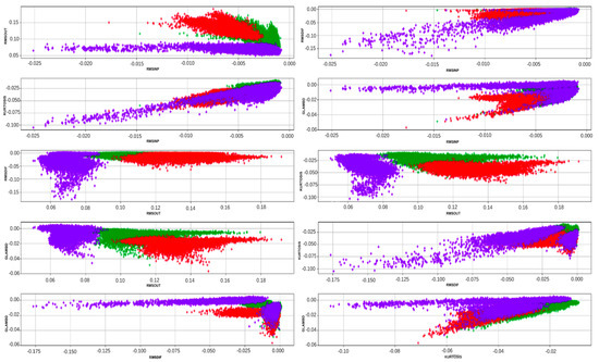
Figure 1. Scatter plot of five different correlation attributes.

Some attributes show a good level of visual separation between the different types of filtering, particularly the harsh one. The clusters of attributes for the mild and the optimal filtering are close as they reflect the observation made earlier about the subtle differences between the two types of filtering.

The environmental and acquisition constraints do not change significantly around a local spatial neighborhood and this implies that the quality of the denoising does not change either. As a result, we suppose that filtered signal quality (i.e., optimal, harsh, and mild) corresponding to the N successive shots in one swath of data is spatially co-located. Therefore, we decided to merge the attributes of all the shots of a given swath with the attributes of their $m=\frac{N}{2}$ previous neighbors and $m=\frac{N}{2}$ following neighbors. This technique allows for more robustness for harsh and mild outliers inside one swath of data. The curse of dimensionality generated by the use of a high number of statistical attributes might impact the accuracy of the QC denoise classification process. Therefore, a feature transformation and dimensionality reduction pre-process are required.

3.1. Feature Transformation and Dimensionality Reduction

Feature transformation and dimensionality reduction techniques are essential to find a more separable transformed feature basis, to speed up the classification process, and to avoid overfitting. In the sections below, we detail two main feature transformation techniques: principal component analysis and independent component analysis.

3.1.1. Principal Component Analysis (PCA)

PCA decomposition is useful especially for building uncorrelated features ranked decreasingly according to their amount of energy (i.e., eigenvalues of the attributes correlation matrix). A whitening process is then applied to normalize the principal component’s variance by rescaling the eigenvalues of PCs by their inverse value and performing regularization by adding a small constant to the scaling factor in the case of small eigenvalues to avoid numerical instability.

The scatter plots of the harsh, mild, and prod data points show three potential clusters with polynomial shape. A kernel-based decomposition [10] might be useful to generate more separable attributes and then build a more confident decision space.

We chose to apply a three-degree polynomial-based PCA decomposition [10], as it illustrates the shape of the cross plot of the dataset on its corresponding attributes. The transformed dataset is then feed-forward to a linear and not a polynomial-based support vector machine classifier. Computing the kernel matrix as well as extracting its singular values is fastidious and computationally expensive due to the relatively large dataset.

3.1.2. Independent Component Analysis (ICA)

Independent component analysis decomposition [12] aims to find the independent source from the previously computed uncorrelated features. Multiple ICA algorithms exist and were detailed in the section above. For computational purposes, we chose to use the Fast-ICA algorithm as it is based on an iterative optimization process. Although performing dimensionality reduction by selecting a subset of independent features is possible, we decided to select relevant features based on their statistical energy (i.e., before source separation process), as we are unable to select relevant features from the independent components. Feature transformation and dimensionality reduction are essential pre-processing tasks to speed up the training and validation process and to prevent classification from overfitting caused by the curse of dimensionality. The choice of the classifier is crucial, especially when handling large datasets.

3.2. Classification Methods

Different algorithm performances were analyzed, i.e., multi-layer perceptrons (MLP), instance-based K-nearest neighbor (K-NN), random forest [14], and support vector machine (SVM) [13]. In the sections below, we will detail the different classifier structure used to predict the quality of the seismic data denoising process.

3.2.1. Instance-Based K-Nearest Neighbor

With the K-NN algorithm, it is easy to implement lazy algorithms. It is less time consuming when training but computationally expensive when testing. This strategy provides accurate results by effectively using a richer hypothesis space (i.e., it uses many local linear functions to form its implicit global approximation to the target function). As a result of resource limitations inside the vessels, instant prediction of the production dataset might be computationally unaffordable.

3.2.2. Random Forests

Random forest [14] is a very powerful classifier. The trees of the forest, and more importantly their predictions, need to be uncorrelated. To achieve this requirement, we chose the bootstrap aggregation method to perform the distribution of both data points and features over the different trees.

3.2.3. Support Vector Machines

We chose a polynomial kernel SVM based on visual assessment of the scatter plot of data points projected on its PCs. The degree of the polynomial kernel was optimized using a grid-search method and the validation accuracy as a metric for maximization.

Many approaches exist when it comes to performing a multiclass support vector machine. We decided to implement and analyze the classification performance and the computation expenses of both one-vs.-one and one-vs.-the-rest-based support vector machines.

3.2.4. Multi-Layer Perceptronss

MLPs are very efficient, but they are memory and time-consuming classifiers, especially when it comes to adjusting architecture and tuning hyperparameters. As the architecture of the model becomes deeper, the risk of overfitting is higher, especially when training on low feature datasets. Unlike all classifiers discussed previously, which have relatively few tunable parameters, the architecture of MLPs should be adjusted to fit a specific project. This task can be done automatically. In [16,17,18], different strategies for building an autonomous deep learning model were proposed. As a result of computational limitations, these models are trained for only one epoch, which might be appropriate when learning from data streams. This approach does not allow for the optimization process and therefore might skew the architecture growth procedure. In addition, authors in [16,17,18] observed potential forgetting phenomena when evolving the model architecture at the pace of training. We cannot afford to lose information from distant but very informative shots; therefore, we decided to use a more common but secure MLP-building strategy. We proposed a heuristic greedy-based algorithm to find the best neural network structure. It is based on the following fundamental assumption: without regularization, an optimal MLP structure tends to overfit as its depth is increased.

The Figure 2 illustrates the major steps of our proposed binary MLP generator. It is inspired by the Branch and Bound algorithm [20] and aims to build the multi-layer perceptrons model with the least validation cross-entropy error.

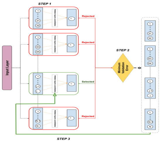
Figure 2. Binary multi-layer perceptrons components overview.

• STEP 1 Several multi-layer perceptrons where trained. Each one consists of a set of permanent layers ( i.e., input layer, layers validated by STEP 2 and the output layer) and one hidden layer candidate. It is composed of 32 to N perceptrons ($64<N<2048$) followed by a $10\%$ dropout layer to avoid overfitting. The validation errors of all the neural network candidates were sent to the Minimum loss processor.
• STEP 2 All the losses received by the STEP 1 are ranked and the neural network candidate with the least validation loss is selected. The remaining mlps are rejected (i.e., they will no longer be processed by the STEP 1).
• STEP 3 Another list of hidden layer candidates is sent back to the STEP 1 and each layer of this list is appended to the final hidden layer of the selected neural network. Then the first STEP is re-operated. All the steps are repeated until the least validation error of the MLP candidates is greater than the least validation error of the previous recursion. At this point, growing the neural network structure becomes inefficient.

Figure 3 details the steps of the one-vs-all binary classification process: The training and the validation set were split into K subsets with equal size following the bootstrap aggregation strategy [21]. The training and validation subsets were converted to $N=3$ binary sets. Then, We applied the previously described greedy binary MLP generator to predict $N.K$ binary decision subspaces. The predicted class members are then fed forward to a voting system that outcomes the class with the majority vote leading to more confident classification results.

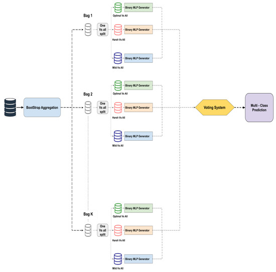
Figure 3. Multi-class MLP generator decision strategy.

4. Experiments

In this section, we detail several experiments using feature extraction, dimensionality reduction techniques, and classification methods.

4.1. Seismic Dataset

The original dataset provided by the off-shore production team consists of several projects (e.g., 4376exm, 4354pgs, 4050eni, 4169tot, and 3920pgs). Each one is a set of filtered data points aligned along different sail lines. To ensure correlation between successive shots in the same sail line, the attribute of each data point is merged with its $Winlen$ previous and successive neighbor, ending up with $(2\times Winlen+1)\times 5$ attributes per data point.

A cross-validation-based accuracy is computed after splitting the projects into five balanced folds in terms of class members to assess the performance of the tested classifiers.

During the testing phase, only two projects were used: 4376exm and 4354pgs. The 4376exm project consists of 40 sail lines (8889 shots): five sail lines for the training and validation process and 35 sail lines for the testing process. The 4354pgs project is composed of 19 sail lines (38,437 shots): five for the training and validation sets and 14 for the testing set.

Figure 4 show three examples of residual seismic data after optimal, harsh, and mild filtering processes of two projects: 4376exm and 4354pgs. The red arrows in the Figure 4 show signal leakage due to the harsh filtering process. The blue arrows illustrate artifacts that are not considered as residual noise.

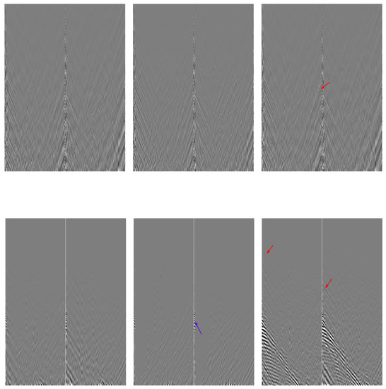
Figure 4. Residual seismic data after prod, mild, and harsh filtering processes (from left to right) of two projects: 4376exm (Top) and 4354pgs (Bottom).

4.2. Feature Transformation and Dimensionality Reduction

4.2.1. Principal Component Analysis

Principal component analysis decomposition was tested on four projects: 4111pgs, 4162pgs, 4374exm, and 4050eni with a $Winlen$ equal to 15, 20, 12, and 25, respectively. As a result of computational limitations, kernel principal component analysis was only tested on three projects (4050eni, 4162pgs, and 4376exm) with a small $Winlen$ value. Even with a small attributes number, performing kernel-PCA decomposition is memory and time consuming because of the large scale of the kernel matrix. To overcome this issue, all matrix operations were performed on a GPU (i.e., Nvidia Tesla V100 16 GB) through the scikit-Cuda library [22], and singular values were approximated using randomized singular value decomposition techniques [23].

4.2.2. Independent Component Analysis

Several techniques were tested to find the unmixing matrix that extracts the independent sources from the principal components. As a result of computational constraints, Infomax- [24] and JADE-based [25] ICA decomposition algorithms could not be assessed (i.e., because of the very large correlation matrices). FastICA [12], which is an iterative-based algorithm, allows for a very fast and less time-consuming decomposition. This algorithm requires a fundamental assumption of the non-Gaussianity of the original features. Therefore, a normal kurtosis hypothesis test was applied to the principal components of all the projects and very low p-value (between 0 and $1\times {10}^{-6}$) outcomes were obtained.

4.3. Classification Methods

The number of nearest neighbors to consider in the instance-based nearest neighbor classifier is crucial. We applied a random search to find the k-value that minimizes the cross-validation error. As a result that the number of classes is odd (three classes), we decided to only consider k not divisible by three to avoid tied votes. We also decided not to use the weighted version of the K-NN algorithm, as the classification process is already robust to noisy data through the attribute reconstruction method.

Although the instant-based algorithm is less time consuming when training, the prediction process is computationally expensive since one needs to scan all the training data to make a decision. Unlike lazy algorithms, the eager classifier training process is computationally less expensive.

The random forest [14] algorithm is one of them. Its hyperparameters were wisely chosen: We used the Gini metric [26] to measure the separability of data points over leaves. In [27], authors concluded that random forest classifiers should include at least 64 trees while not exceeding 128 trees to achieve a good balance between classification performance, memory usage, and processing time. We introduced the early-stopping criterion to choose the appropriate number of trees within the range previously stated. Although the pruning process is required to avoid overfitting, when it comes to using decision tree classifier, the random forest classification method already handles the overfitting issue through features and data bagging.

In contrast, support vector machines and more specifically kernel-based support vector machines are easy-to-train classifiers as they only require kernel space parameter tuning. A grid search-based approach showed that a third-degree polynomial kernel space fits the shape of the clusters of the projected data points. A multiclass support vector machine is based on a combination of binary support vector classifiers with different voting strategies. The one-vs.-one classification strategy is appropriate when handling imbalanced data which is not relevant since all our projects include three categories of filtered shots in the same proportion. Therefore, we decided to use one-vs.-the-rest-based SVM classifier since it achieves good performance with balanced data and is less memory and time consuming (i.e., $(n+1)$ is the binary classifier for the one-vs.-all SVM classifier, whereas it is ${\displaystyle \frac{n(n+1)}{2}}$ for the one-vs.-one SVM classifier).

Unlike all the classifiers we have already analyzed, neural networks are less stable when training due to the relatively high number of tunable parameters and the disparity of the projects in terms of their mean value. The hyperparameters of the neural network have to be wisely chosen. Although RMSprop [28], Adadelta [29], and Adam [30] are very similar algorithms, authors in [30] show that Adam’s bias-correction outperforms RMSprop towards the end of optimization as gradients become sparser. Therefore, in all the following experiments, we trained our MLPs using the Adam [30] optimizer with an initial learning rate tuned to ${10}^{-3}$.

The greedy multi-layer perceptrons model generator described in the previous section is a project adaptive algorithm that builds a local optimal neural network structure. Each neural network candidate is trained for 20 epochs with a categorical cross-entropy loss.

Once the optimal structure was built, we retrained it for 200 epochs and we only saved the weights with a minimum validation error.

4.4. Assessment of the Predicted Quality Control of Seismic Data after Filtering

The QC denoise classification assessment was performed using a combination of three binary-classification evaluation tasks (i.e., harsh, mild, and optimal prediction). Misclassifying shots with signal leakage is considered to be a critical issue due to the high impact of harsh filtering on the relevant signal. As a result, we paid more attention to the harsh classification of a false negative. Undetected harshly filtered shots might be either the result of a highly confident but misleading mild or optimal classifier, a non-confident but correct harsh classifier, or both of them. Therefore, we decided to use two balanced $F_{\beta }$ [31] to assess our binary classifiers: The first, with $\beta =2$, which weighs sensitivity higher than specificity when assessing the harsh classifier performance; the second, with $\beta =0.5$, which weighs specificity higher than sensitivity when assessing the mild or the optimal classification performance.

Despite the relevance of the $F_{\beta }$ [31] and other related statistics-based metrics, visual assessment of the residual signal map by geophysicists remains the most reliable way to assert the seismic data denoise quality control. Therefore, all the filtered test sail line shots, also known as the production lines, were verified by a team of geophysicists.

5. Results and Discussion

In this section, we assess and discuss the different feature transformation and dimensionality reduction strategies. We then compare the classification strategies using the metrics so far described.

5.1. Feature Transformation and Dimensionality Reduction Methods

Table 1 shows the precision, the recall, and the unbalanced F1-score, as well as the computation time of the classification process (i.e., support vector machines) after applying different features and transformation techniques.

Table 1. Classification and time processing assessment of different feature transformation and dimensionality reduction techniques.

Project	$\mathit{F}\mathit{T}$${}^1$ and $\mathit{D}\mathit{R}$ ${}^2$ Methods	${\mathit{F}}_{\mathit{\beta }}$ Score [31]			Processing Time (s)
		Optimal	Harsh	Mild
4376exm	whitening	93.1	99.3	98.4	130
	PCA	93.8	100	98.2	100
	Kernel PCA	91.5	98.3	97.3	5300
	ICA	87.1	99.0	97.3	540
4354pgs	whitening	95.7	91.2	90.3	1432
	PCA	96.8	93.6	90.5	1054
	Kernel PCA	91.5	91.7	88.9	10321
	ICA	95.0	90.9	84.3	2630

¹ Feature transformation, ² dimensionality reduction.

Table 1 illustrates the processing time of different feature transformation techniques and shows the classification performance of an SVM classifier trained on those transformed data. The principal component analysis was found to be less time consuming and generate more separable features. The whitening process consisting of a simple standard scalar operation achieves classification performance close to the PCA decomposition since it encompasses more informative data. This justifies the small computational time of the PCA decomposition compared to the whitening process. The processing time metric includes feature transformation pre-processing and classification time. The PCA decomposition itself is more time consuming than a simple standard scalar operation. As a result, principal component analysis significantly reduces the classification time which confirms our intuition. Unexpectedly, the independent components analysis decomposition [12] led to relatively poor classification performance. Figure 5a,b illustrate the non-correlation between the features of independence and class separability which impacts the decision boundaries generation.

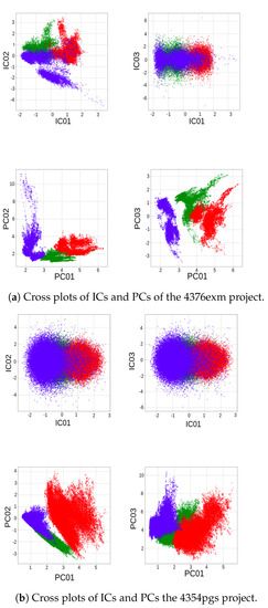
Figure 5. Cross plots of the first, second, and third independent and principal components of the 4376exm and 4354pgs projects.

Principal component analysis decomposition led to the best classification performance while limiting the computational expense (i.e., processing time). Therefore, PCA pre-processing was applied at the beginning of each QC prediction experiment.

5.2. Classification Algorithms

In this section, we evaluate the efficiency of instance-based nearest neighbor, the support vector machines, the random forest classifier, and the MLP predictor in terms of classification performance and computational costs.

According to Table 2, the instance-based nearest neighbor classifier performed relatively poorly in terms of classification compared to the eager algorithms. multi-layer perceptrons outperformed the support vector machine and random forest for the harsh-vs.-the-rest and optimal-vs.-the-rest classification problem of project 4376exm, while the support vector machine achieved the best classification performance of the 4354pgs project. Although the classification assessment metrics (precision, recall, F1-score) are crucial to evaluate and compare the performance of the models, the computational costs are a key parameter, especially when it comes to processing the quality control of the filtered seismic data inside the vessels. Therefore, we only considered models with relatively low training and prediction latency.

Table 2. Classification performance of different models applied to two projects (4376exm and 4543pgs).

Project	Classifier	${\mathit{F}}_{\mathit{\beta }}$ Score [31] (%)
		Optimal	Harsh	Mild
4376exm	Support Vector Machine	95.1	93.7	93.3
	Random Forest	93.4	94.7	99.3
	multi-layer perceptrons	95.5	95.6	98.0
	Instance-based Nearest Neighbors	71.6	89.7	82.4
4354pgs	Support Vector Machine	93.6	99.7	90.9
	Random Forest	91.7	97.8	83.7
	multi-layer perceptrons	93.5	99.2	90.9
	Instance-based Nearest Neighbors	87.6	92.1	91.4

The processing time of one classification approach includes the model hyperparameters and structure tuning procedure as well as the learning process. multi-layer perceptrons and instance-based nearest neighbor are relatively more time consuming than the other classifiers (i.e., support vector machine and random forest) which are affected by their tuning and learning process: The multi-layer perceptrons structure generation is fastidious due to the high but a necessary number of epochs per iteration (20 for tuning and 200 for learning). Indeed, we observed that when decreasing the number of epochs, the MLP candidate was underfitted, which impacts the relevance of the optimal number of perceptron selection for each layer. The data fitting process was relatively less time consuming due to the low number of batches: 544 batch for the 4543pgs project and 276 batches for the 4376exm project. Each batch consists of 50 data points. The training phase of the instance-based nearest neighbor classifier was unexpectedly more time consuming than the prediction phase due to the nearest neighbors considered in the tuning process. The memory usage observations confirm the conclusion derived from the analysis of the Processing time of both the training and prediction phase of each classifier: To find the suboptimal MLP structure, the generator algorithm tested several architecture candidates, each one consisting of between 4099 and 1,082,371 trainable parameters. We ended up with hundreds of millions of generated parameters and hence a very memory consuming process. Given the results stated in Table 3, the support vector machine achieved the best trade-off between computational expenses reduction and good classification performance. Therefore, we chose it for the testing phase. We had already statistically assessed the feature transformation and classification techniques and decided to proceed with principal component analysis decomposition while keeping only $80\%$ of the total energy as a pre-processing step, as well as choosing the SVM model with a third-degree polynomial kernel for the classification process. In the next section, we assess the efficiency of our candidate strategy on a massive test set of filtered seismic data. This step was fully assessed by a geophysicist.

Table 3. Processing time and memory usage of different classification strategies of two projects (4354pgs and 4376exm).

Project	Classifier	Processing Time		Memory Usage (kB)
		Training Phase	Prediction Phase
4376exm	Support Vector Machines	15.19	2.98	355.5
	Instance-based Nearest Neighbor	96.8	57.06	6900.5
	Random Forest	15.57	1.68	5223.6
	multi-layer perceptrons	930.4	3.6	31,291.8
4354pgs	Support Vector Machines	633.10	27.88	983.41
	Instance-based Nearest Neighbor	3880.5	27.88	29,606
	Random Forest	128.79	7.69	21,197
	multi-layer perceptrons	9304	6.5	69,350.6

5.3. Geophysical Assessment of QC Denoise Prediction Process

After performing spatial augmentation, feature transformation, dimensionality reduction, and then classification, we predicted the QC map of the remaining testing sail lines of the 4376exm project. Figure 6 shows the final QC-map after achieving the pseudo-labeling and the retraining strategy described in the previous section.

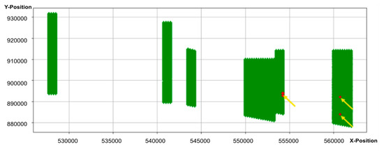
Figure 6. Quality control (QC) map of the 4376exm project.

The QC map was validated by the production team. According to the geophysicists, the shots in the lower right corner of Figure 7a (as shown by the yellow arrows) were misclassified: The detected leakage was a false alarm. We predicted the residual noise (mild filtering) in some production sail lines of the 4354pgs project; these are shown inside the yellow box in the figure below, which can be seen zoomed in in Figure 7b. The shots denoted by the yellow arrows and predicted as harshly filtered are false alarms.

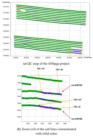
Figure 7. Assessment of the QC prediction of the 4354pgs project.

Our predictions of mild noise in some shots, especially those belonging to the 060 sail lines were validated by the geophysicists of the production team. The red arrows inside Figure 8 highlights the mild noise inside one seismic image of the 60 sail line.

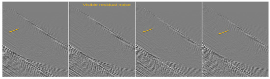
Figure 8. Filtered seismic image of the 60 sail line.

6. Conclusions

Here, we demonstrated that machine learning can automate the QC denoising process using a common pipeline of feature transformation and a dimensionality reduction step followed by supervised learning of the quality control of the filtering process. More attention must be paid to neural networks to reduce their memory usage and time consumption by improving the efficiency of the automotive neural network generation strategy. The spatial correlation between successive shots provided valuable information about the QC denoising process of a sequence of shots; therefore, this must be further explored and evaluated.

References

- Mandelli, S.; Lipari, V.; Bestagini, P.; Tubaro, S. Interpolation and Denoising of Seismic Data Using Convolutional Neural Networks. arXiv 2019, arXiv:cs.NE/1901.07927. [Google Scholar]
- Hearst, M.A.; Dumais, S.T.; Osuna, E.; Platt, J.; Scholkopf, B. Support vector machines. IEEE Intell. Syst. Their Appl. 1998, 13, 18–28. [Google Scholar] [CrossRef]
- Villalba-Diez, J.; Schmidt, D.; Gevers, R.; Ordieres-Meré, J.; Buchwitz, M.; Wellbrock, W. Deep Learning for Industrial Computer Vision Quality Control in the Printing Industry 4.0. Sensors 2019, 19, 3987. [Google Scholar] [CrossRef] [PubMed]
- Küstner, T.; Gatidis, S.; Liebgott, A.; Schwartz, M.; Mauch, L.; Martirosian, P.; Schmidt, H.; Schwenzer, N.; Nikolaou, K.; Bamberg, F.; et al. A machine-learning framework for automatic reference-free quality assessment in MRI. Magn. Reson. Imaging 2018, 53, 134–147. [Google Scholar] [CrossRef]
- Jakkampudi, S.; Shen, J.; Li, W.; Dev, A.; Zhu, T.; Martin, E.R. Footstep detection in urban seismic data with a convolutional neural network. Lead. Edge 2020, 39, 654–660. [Google Scholar] [CrossRef]
- Yu, S.; Ma, J.; Wang, W. Deep learning for denoising. Geophysics 2019, 84, V333–V350. [Google Scholar] [CrossRef]
- Bekara, M.; Day, A. Automatic QC of denoise processing using a machine learning classification. First Break 2019, 37, 51–58. [Google Scholar] [CrossRef]
- Spanos, A.; Bekara, M. Using Statistical Techniques to Improve the QC Process of Swell Noise Filtering. In Proceedings of the 75th EAGE Conference & Exhibition Incorporating SPE EUROPEC, London, UK, 10–13 June 2013; European Association of Geoscientists & Engineers: London, UK, 2013. [Google Scholar] [CrossRef]
- Bekara, M. Automatic Quality Control of Denoise Processes Using Support-Vector Machine Classifier. In Proceedings of the Conference Proceedings, 81st EAGE Conference and Exhibition, London, UK, 3–6 June 2019; pp. 1–5. [Google Scholar] [CrossRef]
- Scholkopf, B.; Smola, A.; Müller, K.R. Kernel principal component analysis. In Advances in Kernel Methods—Support Vector Learning; MIT Press: Cambridge, MA, USA, 1999; pp. 327–352. [Google Scholar]
- Rahman, M.; Khan, M.J.; Adeel Asghar, M.; Amin, Y.; Badnava, S.; Mirjavadi, S.S. Image Local Features Description Through Polynomial Approximation. IEEE Access 2019, 7, 183692–183705. [Google Scholar] [CrossRef]
- Hyvärinen, A.; Oja, E. Independent component analysis: Algorithms and applications. Neural Netw. 2000, 13, 411–430. [Google Scholar] [CrossRef]
- Milgram, J.; Cheriet, M.; Sabourin, R. “One Against One” or “One Against All”: Which One is Better for Handwriting Recognition with SVMs; ETS-Ecole de Technologie Superieure: Montreal, QC, Canada, 2006. [Google Scholar]
- Breiman, L. Random forests. Mach. Learn. 2001, 45, 5–32. [Google Scholar] [CrossRef]
- Adnan, M.N.; Islam, M.Z. One-vs-all binarization technique in the context of random forest. In Proceedings of the European Symposium on Artificial Neural Networks, Computational Intelligence and Machine Learning, Bruges, Belgium, 22–24 April 2015; pp. 385–390. [Google Scholar]
- Inoue, H.; Narihisa, H. Efficiency of Self-Generating Neural Networks Applied to Pattern Recognition. Math. Comput. Model. 2003, 38, 1225–1232. [Google Scholar] [CrossRef]
- Pratama, M.; Za’in, C.; Ashfahani, A.; Ong, Y.S.; Ding, W. Automatic construction of multi-layer perceptron network from streaming examples. In Proceedings of the 28th ACM International Conference on Information and Knowledge Management, Beijing, China, 3–7 November 2019; pp. 1171–1180. [Google Scholar]
- Ashfahani, A.; Pratama, M. Autonomous Deep Learning: Continual Learning Approach for Dynamic Environments. In Proceedings of the 2019 SIAM International Conference on Data Mining, Calgary, AB, Canada, 2–4 May 2019; pp. 666–674. [Google Scholar] [CrossRef]
- Chen, C.C.; Chu, H.T. Similarity Measurement Between Images. In Proceedings of the 29th Annual International Computer Software and Applications Conference (COMPSAC’05), Edinburgh, UK, 26–28 July 2005; Volume 2, pp. 41–42. [Google Scholar] [CrossRef]
- Kolesar, P.J. A branch and bound algorithm for the knapsack problem. Manag. Sci. 1967, 13, 723–735. [Google Scholar] [CrossRef]
- Breiman, L. Bagging predictors. Mach. Learn. 1996, 24, 123–140. [Google Scholar] [CrossRef]
- Givon, L.E.; Unterthiner, T.; Erichson, N.B.; Chiang, D.W.; Larson, E.; Pfister, L.; Dieleman, S.; Lee, G.R.; van der Walt, S.; Menn, B.; et al. Scikit-Cuda 0.5.3: A Python Interface to GPU-Powered Libraries. 2019. Available online: https://www.biorxiv.org/content/10.1101/2020.07.30.229336v1.abstract (accessed on 20 October 2020).
- Martinsson, G.; Gillman, A.; Liberty, E.; Halko, N.; Rokhlin, V.; Hao, S.; Shkolnisky, Y.; Young, P.; Tropp, J.; Tygert, M.; et al. Randomized methods for computing the Singular Value Decomposition (SVD) of very large matrices. In Works. on Alg. for Modern Mass; Data Sets: Palo Alto, CA, USA, 2010. [Google Scholar]
- Nadal, J.P.; PARGA, N. Sensory coding: Information maximization and redundancy reduction. In Neuronal Information Processing; World Scientific: Singapore, 1999; pp. 164–171. [Google Scholar]
- Rutledge, D.N.; Bouveresse, D.J.R. Independent components analysis with the JADE algorithm. TrAC Trends Anal. Chem. 2013, 50, 22–32. [Google Scholar] [CrossRef]
- Dagum, C. Decomposition and interpretation of Gini and the generalized entropy inequality measures. Statistica 1997, 57, 295–308. [Google Scholar]
- Oshiro, T.; Perez, P.; Baranauskas, J. How Many Trees in a Random Forest? In Proceedings of the International Workshop on Machine Learning and Data Mining in Pattern Recognition, New York, NY, USA, 19–25 July 2012; Volume 7376. [CrossRef]
- Tieleman, T.; Hinton, G. Lecture 6.5-rmsprop: Divide the gradient by a running average of its recent magnitude. Coursera Neural Netw. Mach. Learn. 2012, 4, 26–31. [Google Scholar]
- Zeiler, M.D. Adadelta: An adaptive learning rate method. arXiv 2012, arXiv:1212.5701. [Google Scholar]
- Kingma, D.P.; Ba, J. Adam: A method for stochastic optimization. arXiv 2014, arXiv:1412.6980. [Google Scholar]
- Baeza-Yates, R.; Ribeiro-Neto, B. Modern Information Retrieval; ACM Press: New York, NY, USA, 2011; pp. 327–328. [Google Scholar]
Publisher’s Note: MDPI stays neutral with regard to jurisdictional claims in published maps and institutional affiliations. |
© 2020 by the authors. Licensee MDPI, Basel, Switzerland. This article is an open access article distributed under the terms and conditions of the Creative Commons Attribution (CC BY) license (http://creativecommons.org/licenses/by/4.0/).