Abstract
The orientation and relative magnitudes of paleo tectonic stresses in the western central region of the White Mountains of New Hampshire is reconstructed using the direct inversion method of fault slip analysis on 1–10-m long fractures exposed on a series of road cuts along Interstate 93, just east of the Hubbard Brook Experimental Forest in North Woodstock, NH, USA. The inversion yields nine stress regimes which identify five tectonic events that impacted the White Mountain region over the last 410 Ma. The inversion method has potential application in basin analysis.
1. Introduction
Previous studies have shown fault slip analysis at the outcrop scale provides a means to deduce the orientation of the principal stress fields and their evolution through successive tectonic events [1,2,3,4,5,6,7]. Additional information obtained from other structures, such as joints [8] tension gashes, and stylolites [9], is also important but will not be presented here. In this paper, we define a fault as simply a parting in rock with no claim whether it formed as a Mode 1 (opening), Mode 2 (shearing), or Mode 3 (tearing) [10]. If a fault shows shear offset (Mode 2). The input for fault slip analysis is field data collected on the surfaces of individual faults which includes the orientation of the, slip direction, and sense of slip. The latter two are determined by one or more of the following displacement indicators visible on the fault surface: slickensides, asperity ploughing, slickolite spikes, crescent marks, the growth of mineral patches on the lee side of hills on a rough fault surface, mineral fibers and steps, and Reidel shears [11].
The basic assumptions behind fault slip analysis are that: (1). conjugate fault sets result from a single brittle deformation event, and (2). slip on a fracture surface occurs in the direction of maximum resolved shear stress. The first step in the analysis consists of reconstructing the “reduced stress tensor”. The reduced stress tensor differs from the actual stress tensor only in that the absolute magnitudes of the principal stresses: σl (maximum compressional stress), σ2 (intermediate stress), and σ3 (minimum stress) are not determined, only their relative magnitudes. However, the relative magnitude, order, and orientation of the three principal stresses are the same as for the actual stress tensor and enable one to define the directions of compression and extension which prevailed during tectonic events. Knowing the stress state, one determines the shear stress and hence the slip orientation expected on any plane. The first attempt at formulating and solving the inverse problem was [12]. Numerical methods have since been developed for reconstructing paleo-stress orientations from fault slip data. In the general case illustrated in this paper, any planar discontinuity in a rock may be activated as a fault. The discontinuity may be either a pre-existing fracture activated or reactivated (inherited fault) by the tectonic stress. The basic properties of the reduced stress tensor and its determination is summarized below. The indicators of the direction and sense of shear on a discontinuity reactivated in shear is to collect and analyze fault slip data. The method of direct inversion used in this paper can be found in [1,2,3,4,5,6,13,14] and in [15].
2. Geologic and Tectonic History of the Southwestern White Mountain Region
The bedrock geology of the study site and Hubbard Brook valley has been mapped (sheet 1) at a scale of 1:12,000 [16] and at a scale of 1:10,000 [17]. The study site is also included in earlier bedrock maps [18,19] and at a scale of 1:250,000 [20]. The bedrock underlying the study site (Figure 1) consists of metamorphic rocks intruded by igneous rocks and belongs to the Central Maine Trough [20]. The metamorphic rocks of the Rangeley and Perry formations were deposited as sandy, clay-rich marine sediments [21] on a continental shelf, rise, and abyssal plain of the Rheic Ocean [22] over a time spanning the Silurian (approximately 443–428 Ma). These sediments were then buried and multiply folded by at least two deformation episodes [17] in the Acadian orogeny (early Devonian, 410–390 Ma), as the Rheic Ocean closed and Avalon collided with eastern North America. At this time, the rocks were metamorphosed to the lower sillimanite grade (approximately 600 °C and 4 kb pressure, equivalent to a burial depth of approximately 15 km), which resulted in local melting (migmatization). At approximately 410 Ma, these rocks were at or near the conditions of maximum pressure and temperature and were intruded locally by the southern portion of a large pluton of the Kinsman granodiorite of the New Hampshire plutonic series. The Kinsman granodiorite underlies most of the western half of the Hubbard Brook Valley immediately to the west of the study site [16] see Figure 1. Near the bottom of Figure 1 is a low angle thrust called the Thornton Fault on [20]. This fault thrusts older Silurian rocks over younger Devonian rocks. The fault is cutoff by and therefore must be older than the intrusion of the Kinsman Granodiorite, but younger than the Littleton Formation. This fault extends below the study site and below the Rangeley Formation at the study site. This fault may have formed during Tectonic Event 1 in Table 1 and Table 2. During the late Devonian (370–365 Ma) the metamorphic rocks and the Kinsman intrusion were multiply intruded by small tabular dikes and small discordant bodies of Concord granite, also of the New Hampshire plutonic series. The Concord granite is shown on the map at a scale of 1:200 [16] and in well logs [23], but is not shown in Figure 1 which is modified from the map of [20] (scale of 1:500,000).
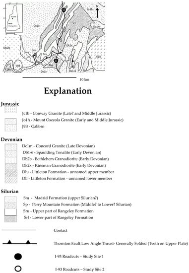
Figure 1.
Bedrock geologic map for the area immediately surrounding the two study sites along the I-93 roadcuts in Woodstock, NH, USA. (After [20], sheet 1). Location map is shown in upper left. The study site is located in the Lower Rangeley Formation.

Table 1.
Results of inversions for nine tectonic regimes based on the direct inversion method [4] with additional refining process [13]. Reg. = reference number of regime, also referred to in Table 2. MIFL = the control parameter, indicates the minimum individual fit level finally retained (see the term ω in [13] for detailed discussion of MIFL). NA = number of fault planes found acceptable at this level of fit. NR = number of fault planes rejected. The stress tensor obtained is characterized by the trends and plunges of the three principal stress axes, σ1, σ2, and σ3, and by Φ = (σ2 − σ3)/(σ1 − σ3), the ratio of the principal stress differences where 0 ≤ Φ13 [2]. υm = average value of the main estimator [4], τ*m = ratio of the average shear stress to the maximum shear stress. αm = average value of the calculated shear-actual slip angle.
Table 2.
Tectonic paleo-stress chronology including: tectonic events (compressional or extensional), relative chronological order, regime number, fault type, and orientation of the three principal stresses, as determined by fault-slip analysis in the present study. The time ranges are from the published literature where known tectonic events in the region have been dated as presented in Section 2 above. The orientation of the principal stresses for each tectonic event has one oriented vertical and two horizontal with azimuthal angles as shown.
The Alleghenian orogeny (325–260 Ma) created the Appalachian Mountains principally by collision with North Africa. While it may not have resulted in large scale deformations at the study site, it was strong enough to create or reactivate fractures.
From early to late Jurassic (194 to 155 Ma) the are immediately to the east and north of the study site was a region of extensive granitic intrusion expressed by the huge batholiths and ring dikes of the White Mountain plutonic/volcanic series [24]. During that time or possibly later (130 to 100 Ma), the metamorphic and igneous intrusive rocks at the study site were intruded by tabular diabase dikes, emplaced as part of continental rifting associated with the opening of the present Atlantic Ocean basin.
From the time of the Acadian Orogeny to the present, erosion and uplift have brought the bedrock from a depth of approximately 15 km to at or near the Earth’s surface. The last episode of deformation was the loading and unloading of the bedrock by the advance and retreat of multiple glacial ice sheets over this region in the past 100,000 years [25]. Reconstructions of the thickness of the Laurentide ice sheet yield a glacial ice loading and unloading of three kilometers for New England [26].
Based upon the orientation of glacial striations, the last Wisconsin Ice sheet moved over the study site from WNW to the ESE [16]. At the last glacial maximum 14,000 years ago, the minimum thickness of the ice at the study site was approximately 1.6 km [27]. The glaciers swept away the thick loess, soils and vegetation that previously covered the bedrock. In some places, the advancing glacial ice plucked automobile-sized blocks from the leeward side of the ridges and small hills in the Hubbard Brook valley. Throughout the valley, glacial ice and water carved and polished the top of the bedrock to a smooth, undulating surface. Finally, as the ice sheet melted in place, the rock debris within the glacier, worked by rivers and streams on top of, within, and beneath the melting ice, was deposited as discontinuous layers on top of the bedrock surface with thickness increasing from 0 at and near the ridge crests and stream beds to as much as 50 m in the lower part of the valley [27]. Because of the glaciation-related erosion, the present-day rock condition of bedrock exposures is extremely fresh, which makes our study of brittle structures much easier than if it were weathered rock.
The geology and faults studied in this report are exposed in roadcuts along Interstate 93 (Figure 2) which were mapped at a scale of 1:200 by [16] sheet 2. All naturally occurring fractures greater than one meter in scale are shown on the map. Fracture orientation, trace length, aperture, surface roughness, and interconnectedness were measured and analyzed [16,28]. The compositional variability in the schist persists to the millimeter scale. The schist has a well-defined foliation, which has been refolded at least twice, and the foliation can be highly variable at length scales less than a meter. At larger scales, the foliation strikes from 25 to 45 degrees east and dips steeply to the southeast, consistent with the regional tectonic fabric.
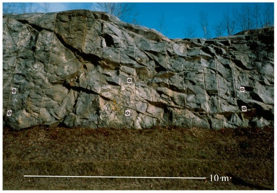
Figure 2.
Photograph of a N5E striking roadcut exposure at the study site on I-93 containing NE striking, SE dipping faults included in this study. Note, most of the faults fractures exhibit dark planar surfaces. The rock type is primarily Concord granite (dark gray) with a Lower Rangeley schist block (light grey/white) exposed to the right of center above where the grass meets the bedrock and between the first and fourth drillhole from the left side of the photo. The subvertical lines are drill holes used in blasting the roadcut surface. Targets were used for rectification of photographs on which the geology and fractures were mapped by [16] (sheet 2).
The granitic rocks intrude the schist in the form of small tabular dikes and large anastomosing fingers ranging from 1000′s of meters to the meter scale. The intrusion was prolific, and granitic rocks account for approximately 50% of the rock area mapped in the road cuts, Figure 2 [16] sheet 2. and in the 40 boreholes (totaling 4.6 km of wellbore) drilled in the Mirror Lake watershed, located at the eastern end of the Hubbard Brook valley [23]. Changes in lithology between granite and schist occurs every 5–9 m in the roadcuts [16] and the boreholes [23].
Bedrock fractures in the roadcuts, natural outcrops and the bedrock wells include joints (formed as Mode 1 fractures), faults (formed as Mode 2 fractures), and reactivated faults and joints. Fractures formed prior to the maximum burial and temperature (410–390 Ma) would have been destroyed by metamorphic recrystallization. We therefore assume that all the fractures that we observe in outcrop were formed after the peak metamorphic event at approximately 390 Ma. It is not possible to determine the age of fracture formation or reactivation using relative or radiometric dating. The brittle tectonic activity since 390 Ma could result from events during the Alleghenian orogeny (Permian, 299 to 251 Ma) and to younger tectonic events, such as the extension related to the opening of the northern Atlantic ocean approximately 200–175 Ma or to the glaciation-deglaciation cycles of the Quaternary (2.6 Ma to present) [27]. Little evidence for the age of brittle events can be obtained from stratigraphy or rock dating, although thin (~1 m) NE-SW striking diabase dikes occur in the study site during the early Jurassic 200–146 Ma may be a brittle episode related to the opening of the Atlantic Ocean. Large numbers of fracture surfaces display syntectonic mineral infill or fiber growth. Because syntectonic minerals like quartz could not develop during the brittle events at very shallow depth, such mineralization indicates that most of the brittle tectonic activity that produced the fault slips took place at depths up to 15 km., and hence is related to tectonic episodes that predate the glaciation-deglaciation events
3. Data Collection and Stress Inversion Method of Analysis
Two hundred and eight fault-slip data were collected at roadcuts in bedrock at two locations on Interstate-93 in Woodstock, New Hampshire as shown in Figure 1. The first location includes four sub-parallel vertical roadcut faces approximately 40 m apart, whose bedrock geology and fractures had been previously mapped [16]. The second location is a roadcut on the east side of the northbound lane of I-93, 1.3 km north of the first location. Figure 2 is a photograph of a section of a portion of roadcut at location 1 showing NE striking, SE dipping fractures in the Concord granite 370–365 Ma.
Faults were easily identifiable in the roadcuts, most of them bearing slickensides resulting from slip-parallel quartz growth. Numerous faults show minor (~1–2 mm) but clearly observable offsets of cleavage, schist-granite contacts, quartz-pegmatite veins, and along contacts of the diabase dikes and the schist and granite. Evidence of slip-parallel quartz growth was common. The strike and dip of the fault plane, the rake of the slickenside lineations, and the sense of relative offset were measured for each observable fault. The faults were numbered. All types of fault slips were found: dip-slip, strike-slip and oblique slip, with normal, reverse, right-lateral and left-lateral components of motion. This variety of fault slips indicates polyphase brittle tectonism, which was confirmed by differences in mineral fillings. The inferred tectonic regime/relative chronology (by number) and level of certainty, the roadcut location, and the fracture number on [16], were all noted. All the information recorded is listed in Appendix A Table A1.
Particular attention was paid to determination of the sense of motion on each fault. A variety of criteria were used, including: (1) offset of granite-schist and other metamorphic boundaries, (2) mineral growth along the slip direction, (3) presence of rough and polished facets along the fault surface, (4) asymmetrical striation markers, (5) striation-related micro-veins, (6) offsets of older fractures or veins, (7) presence of small Riedel’s shear fractures, mainly R in type. Where possible, these criteria were cross-checked. As a result, three levels of certainty were considered concerning the senses of motion (see Appendix A, Table A1). The letter C refers to a slip sense that could be determined with certainty in the field, based on one or several unambiguous criteria. The letter P indicates that the slip sense is considered probable, which means that despite good observation some ambiguity could not be removed. The letter S refers to a poorly recorded sense of motion, in the absence of reliable criterion or with conflicting criteria. In that case an inferred “supposed” sense of motion was attributed, based on both the low-quality criterion (if any) and the behavior of the neighboring faults with well-recorded sense of motion and similar dip direction, attitude, and slip orientation.
Many faults were associated in conjugate or Riedel’s type patterns with particular symmetries. Fault subsets were defined based on common geometry in terms of fault attitude, slip orientation and sense, fault dip direction, relation to other faults, and mechanical consistency. The relation between conjugate fault systems and stress has been highlighted by Daubrée’s experiments [29] and Anderson’s analysis [30]. In addition, Riedel’s shears [11] often explain the relationships between faults at different scales.
Most fault slip data in the outcrops studied could not be interpreted in simple geometrical terms, because they resulted from reactivation of earlier faults or mechanical discontinuities (older faults, joints, veins, cleavage, contacts between rock types, etc.). Such inherited faults may have various attitudes oblique to all stress axes, contrary to the “newly formed” faults discussed above, which generally contain one principal stress axis and form symmetrical systems. For this reason, we undertook systematic inversion of the fault slip data to reconstruct the stress regimes. Such inversions are based on consideration of the stress-slip relationships proposed by [31,32], which were used by [12], who first addressed the inverse problem in their pioneering work. Later studies demonstrated that the basic assumptions underlying the method were acceptable in the first approximation and well accounted for actual slip distribution (e.g. [2,3]), and numerical modeling experiments showed that deviations from the model are significant but remain statistically minor with regard to other sources of uncertainty [33].
The direct inversion method’ used here is based on a least-square minimization, with a criterion called υ (upsilon) that depends on both the angle between the calculated shear and the actual slip, and the shear stress amplitude relative to maximum shear stress. For details, the reader is referred to the paper that describes this method [4]. We also use a robust refining process that was not described in the original formulation of the method but is presented in the use of another method especially designed for the stress inversion of earthquake focal mechanisms [13]. This additional process was facilitated by the negligible runtime of the inversion method, which involves analytical means instead of numerical search. A crucial parameter is the minimum fit level required for defining acceptable data. We use a scale from −100% (total misfit) to 100% (perfect fit). The lowest bound involves maximum shear stress acting in the direction opposite to slip. At the highest bound, the shear stress is also maximum but acts in the same direction and sense as the slip. A zero value indicates that slip occurs with shear stress perpendicular to slip, as the limit between consistent and inconsistent senses of motion. Note that this minimum fit level is linearly related to the RUP % estimator defined by [4], the values −100% and +100% corresponding to the values 200% and zero (respectively) in the RUP estimator and differs from the ω estimator defined by [13].
To determine a stress regime, υ is minimized as a function of the four unknowns that describe a reduced stress tensor: the orientations of the three principal stress axes and the ratio Φ = (σ2 − σ3)/(σ1 − σ3). One obtains the smallest slip-shear angles and the largest possible shear stresses that can simultaneously exist for all the data taken together.
The real data dispersion, which depends on complex geological factors, is larger than the angular uncertainty of about 5° in our field data collection. To determine whether a stress inversion is significant or not, we use an iterative refining process that involves successive inversions with a progressively increasing demand for good individual fits. This process allows determination of the level of data rejection consistent with the data accuracy.
4. Results
Based on consideration of relationships between fault slips (crosscutting relationship, reactivation of fault surface, etc.), spatial association between faults (e.g., conjugate patterns) and syntectonic mineral growth (e.g., quartz fibers), and taking into additional account the mechanical consistency within each subset of fault slips, it was possible to separate nine data subsets (regimes), as listed in Table 1 below.
The number of Regimes is large (9). High confidence can be placed in the definition of the regimes themselves, their sequential order, and especially the directions of compression and extension of the inferred stress tensor. A second step involves grouping the Regimes into tectonic Events where the known regional tectonics coincides with the direction of the principal stresses and the time sequence of known regional tectonic events. The grouping into Events is shown in Table 2 and discussed below.
Each Regime is depicted on a lower hemisphere equal area projection below showing the great circles of each of the fault planes determined. Arrows indicate the slip on the fault planes. A separate companion plot displays the same arrows and the poles to the fault planes (open circles) and the trend and plunge of the intermediate stress (σ2). Arrows pointing toward the center of the projection indicate compression. Arrows pointing to the perimeter of the projection indicate extension. Solid circles with two arrows pointing in opposite directions indicate the sense of strike-slip movement. Those with no arrowheads have an indeterminate sense of movement.
4.1. Event 1—Regime 1
This regime is characterized by reverse faults compatible with a NW-SE compression (Figure 3). The frequent presence of quartz veins and along-slip quartz growth indicate that slip probably occurred close to the ductile-brittle transition. The relatively deep and hot character of this tectonic deformation suggests that this event is the oldest event.
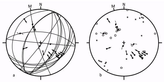
Figure 3.
Regime 1. Lower Hemisphere Equal Area projection of (a) great circles of fault plane orientation, and (b) poles to fault planes (open circles) and (*) the calculated trend and plunge of σ2. The arrows indicate the rake of slickenlines on the fault planes and point in the direction of slip. Arrows pointing toward the center of the projection indicate compression, those pointing away from the center indicate extension. Solid circles with two arrows pointing in opposite directions indicate the sense of strike-slip movement. Those with no arrowheads have an indeterminant sense of movement. M = magnetic north, N = true north.
The stress inversion of fault slip data for this data subset shows that for a reasonable threshold, MIFL = 40%, only 2 of the 19 fault slip data are considered unacceptable. Similar solutions were obtained for minimum individual fit levels of 20% (no data being eliminated) or 40% (4 data eliminated). The stress regime determined is thus stable.
The calculated stress regime indicates a nearly horizontal compression that trends 133° N. The stress axes σ2 and σ3 are oblique, with plunges of 45°, in agreement with the low value, 0.13, for the ratio Φ = (σ2 − σ3)/(σ1 − σ3). This low Φ reveals σ2 and σ3 are closer in magnitude than either is to σ1. The solution cannot be considered very accurate because the number of acceptable fault planes inversions is small (17). The direction of compression is constrained within ±10 degrees, but the values of Φ and the attitudes of stress axes σ2 and σ3 may vary widely as a function of data removal within this set. In summary: the oldest brittle tectonic episode that we can recognize corresponds to a NW-SE compression that reactivated deep fractures in reverse faulting.
4.2. Event 2—Regimes 2 and 3
In contrast to Regime 1, both Regimes 2 and 3 are dominated by normal fault extension (Figure 4). Most are dip-slip, which suggests a low level of structural inheritance and reactivation of earlier structures. Most fault surfaces are planar with relatively steep dips, which suggests that they developed at shallower crustal levels than the reverse faults of Regime 1. However, the gentle dips of some of the normal faults suggests the reverse faults of Regime 1 have been reactivated as normal slips. Note that the dominate trend of normal faults in Regime 3 are the same as for the reverse faults of Regime 1 (e.g., the fault poles are similar). Syntectonic quartz is common on the surfaces of these inherited normal faults, with the quartz probably inherited from Regime 1.
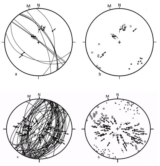
Figure 4.
Regime 2 (top) and Regime 3 (bottom). Lower Hemisphere Equal Area projection of (a) great circles of fault planes; and (b) poles to fault planes (open circles) and of calculated trend and plunge (*) of σ2. Symbols are as in Figure 3.
The two subsets of faults strike at right angles. The normal faults of Regime 2 strike NW-SE. and the normal faults of Regime 3 strike NE-SW. Regime 2 faults indicate NE-SW extension whereas Regime 3 faults indicate NW-SE extension.
The stress inversion of fault slip data for Regime 2 is stable (2 faults rejected at MIFL = 55%, no faults rejected at 20%, and only 4 of the 20 faults rejected at MIFL = 80%), but is only loosely constrained because of the limited number of data (18 acceptable faults). As with Regime 1, the numerical results are good, but the solution is highly dependent on the grouping of data. For example, removing the two nearly vertical faults results in a significantly different solution. The stress regime at MIFL = 55% indicates a 33° ± 10 degrees trending extension with oblique σ1, σ2 and σ3 axes. The σ3 axis plunges 33° NE, which is not surprising in light of the presence of nearly vertical faults with the downthrown side to the northeast. The Φ ratio of 0.46 indicates triaxial stress.
In contrast, the large number of fault slip data in Regime 3 provides a highly constrained stress tensor solution. The solution is stable (13 of 75 faults rejected at MIFL = 40%, 4 at 20% and 20 at 55%). The stress orientations and Φ are similar regardless of the MIFL, which indicates that the stress tensor is well constrained. On the other hand, the slip vectors have a large scatter (Figure 4). The number and geometrical variety of the data are more important than the average of parameter estimates and their standard deviations. Removal of fault slip data does not change the inversion results within the range of uncertainties, which confirms that geometrical constraints on the stress tensor exerted by the variety in fault slip attitudes is more important to a good interpretation. At MIFL = 40% the σ1 axis is nearly vertical and indicates a 110° azimuth of extension (the σ3 axis plunges only 3° to the west). The direction of extension is constrained within ±5 degrees. A Φ ratio of 0.49 indicates typical triaxial stress.
No clear chronological difference could be established between Regimes 2 and 3. The perpendicularity in fault trends and corresponding directions of extensions strongly suggest that these two regimes are linked through a permutation (relative magnitude switch) between the intermediate and minimum principal stresses, σ2 and σ3. These two regimes thus probably belong to a single major extensional event which we identify as Event 2. Because Regime 3 is represented by a much larger number of brittle structures than Regime 2, the dominating direction of extension is inferred to be WNW-ESE (azimuth 110°). A tensor inversion with Regimes 2–3 taken together shows that the influence of the fault slip data from Regime 3 prevails, and the combined tensor solution resembles that of Regime 3. For a MIFL = 30% the Φ ratio is lower (0.35) but the direction of extension is similar (115°). The stability of the solution is much less, which suggests the distinction between Regimes 2 and 3 is in fact significant in terms of stress states, even though both are produced by the same tectonic event. Brittle tectonic analyses have revealed significant changes in stress regimes within a single tectonic episode [4,5,6,13,15]. The duality of stress regimes (2 and 3) may simply result from a permutation between the σ2 and σ3 axes, a common phenomenon in fault tectonics.
Although there remains some indication of ductile-brittle transition for some faults with abundant quartz coating and slip-parallel quartz growth, most Event 2 faults are typically brittle, as shown by both the fault surface characteristics and their steep dips. Relative chronologies with respect to other events show that Regimes 2 (certainly) and 3 (probably) post-dated the Regime 1. Our data thus suggest that the extension of Regimes 2–3 post-dated the compression of Regime 1 and suggests that Regimes 1–3 reflect the oldest two faulting events well represented at the site.
4.3. Event 3—Regime 4
Regime 4 is poorly represented. It is characterized by only a few reverse faults that are compatible with a NE-SW compression. The stress inversion provided stable results, which has little meaning because of the very low number of faults (5). The tensor solution is very loosely constrained. Had more fault slips been identified, the result would have been subject to significant variations. For a MIFL = 45% one of the five faults is considered unacceptable, and the calculated stress regime indicates a 59° compression direction with a nearly vertical σ3 axis and a Φ ratio of 0.44. The direction of compression may however vary within ±20°.
The reverse faults shown in Figure 5 are younger than those of Regime 1, but there is little indication of their age. Two display the same attitude, but different oblique slip vectors from the reverse faults of Regime 1 from which they are inherited.
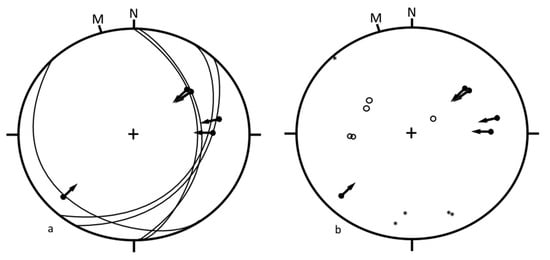
Figure 5.
Regime 4. Lower Hemisphere Equal Area projection of (a) great circles of fault planes and (b) of poles to fault planes (open circles) and of calculated trend and plunge (*) of σ2. Symbols are as in Figure 3.
4.4. Event 3—Regime 5
Regime 5 (Figure 6) is better represented than Regime 4. The stress tensor inversion indicates strike-slip faulting consistent with a nearly E-W compression and N-S extension. These strike-slip faults clearly postdate the reverse faults of Regime 1. The stress tensor inversion is stable (1 of 24 faults rejected at MIFL = 55%, none rejected at 25%, and 7 rejected at MIFL = 70%). Another indication of inversion stability is that the removal of dextral fault slips does not significantly modify the inversion results.
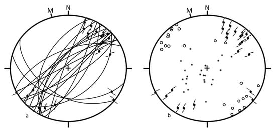
Figure 6.
Regime 5. Lower Hemisphere Equal Area projection of (a) great circles of fault planes and (b) of poles to fault planes (open circles) and of calculated trend and plunge (*) of σ2. Symbols are as in Figure 3.
The stress regime calculated at the MIFL = 55% level is characterized by a nearly horizontal σ3 axis that trends 0° and a gently plunging σ1 axis whose azimuth trends 83°. The direction of extension is not more tightly constrained than ±10 degrees because only 2 left-lateral faults were measured. A typical triaxial stress is indicated by the Φ ratio of 0.50.
Contrary to the typical, most strike-slip faults of Regime 5 are far from vertical. Many of the right-lateral faults dip towards the NW or SE, which suggests that they were inherited from the normal fault planes of Regime 3. Two left-lateral faults have gentle SW dips, which suggests that they were inherited from normal fault planes of Regime 2.
Although the faults of Regime 4 are reverse and the faults of Regime 5 are strike-slip, the directions of compression are similar considering the large angular uncertainty in the trend of compression of Regime 4. For this reason, we combine Regimes 4 and 5 within a single Event 3 that is dominated by a roughly E-W compression and can generate both reverse and the strike-slip faulting. The stress tensor for this combination resembles that for Regime 5 because of the larger number of faults in Regime 5. Unlike the combination of Regimes 2 and 3, the combination of Regimes 4 and 5 shows good stability (1 of 30 faults eliminated for MIFL = 20%, 9 for 55%). But the rejected faults are 2 of the 5 reverse faults of Regime 4, and the individual misfits of the three remaining Regime 4 reverse faults are large. The simplest solution suggests mixing Regimes 4 and 5 are indeed distinct.
For a reasonable fit level of 35% (2 faults rejected), the Φ ratio is 0.43, indicating triaxial stress despite the mixture of strike-slip and reverse faults. The stress regime is characterized by a gently plunging σ3 axis with a trend azimuth of 351° and a nearly horizontal σ1 axis with a trend of 83°. The data indicate stress regimes 4 and 5 belong to a single event dominated by WNW-ESE compression and that a permutation between σ2 and σ3 changes the faulting from reverse to strike slip.
4.5. Event 4—Regimes 6, 7 and 8
The strike-slip faults of Regimes 6–7 are shown and analyzed together (Figure 7). These regimes are dominated by strike-slip faulting. Sixty-nine faults are observed, the largest ones forming typical strike-slip zones composed of two walls on either side of a 1–3 m wide deformed zone with numerous smaller faults, fractures, rotated blocks, and gouge. The strike-slip faults strike approximately NNW-SSE for right-lateral faults, and NNE- SSW for left-lateral ones, indicating N-S compression.
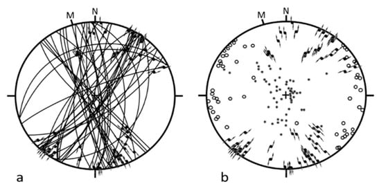
Figure 7.
Regime 6–7. Lower Hemisphere Equal Area projection of great circles of fault planes (a); and (b) of poles to fault planes (open circles) and of calculated trend and plunge (*) of σ2. Symbols are as in Figure 3.
The stress tensor solution is tightly constrained by the large number of the faults and the variety of their orientations (17 faults rejected at MIFL = 45%, 5 at 20%, and 23 at 55%). The stress orientations remain extremely stable as the MIFL increases. In addition, removal of fault slip data does not significantly affect the inversion. The geometrical constraints exerted by the variety in fault slip attitudes are strong. Because a significant overlap in stress trends is present between right-lateral and left-lateral faults, several data displayed incompatible senses of motion. This explains why faults were eliminated even for low levels of MIFL. Separation into two Regimes, 6 and 7, solved this problem and reduced the number of inconsistent senses to zero for each of the stress tensors, but was not retained because no independent qualitative evidence supported a separation of these Regimes.
The stress regime calculated at MIFL = 45% is characterized by gently plunging σ1 and σ3 axes (plunges of 14° and 17° degrees respectively), with a nearly N-S trending, azimuth 188°, compression. This direction of compression is constrained within less than ± 5°. The Φ ratio of 0.45 indicates typical triaxial stress.
Relative chronology data provides good evidence that this major strike-slip event postdated the normal faults of Event 3. Although some strike-slip faults of Regime 6 and 7 have relatively gentle dips suggesting that they were inherited from earlier regimes of reverse and normal faults, most of these strike-slip faults are vertical or steeply dipping, cutting through all pre-existing structures rather than reactivating them. It is likely that several NE-SW trending faults result from right-lateral reactivation of the left-lateral faults of Regime 5, but observation is speculative because of the right-lateral friction that generally destroyed the criteria supporting the evidence of an earlier left-lateral motion.
Regime 8 is represented by only a few dip-slip reverse faults (Figure 8). The relative chronology data indicate that this regime occurred before the Regimes 6 and 7. As with Regime 4, the stress inversion provides very stable solutions, but this stability is not significant because the number of faults is so small. The tensor solution is in fact poorly constrained. For MIFL = 50%, all data are acceptable, and the calculated stress regime indicates an azimuth 330° compression with a nearly horizontal σ1 axis, a steeply plunging σ3 axis and a Φ ratio of 0.23. The direction of compression is constrained within ±20°.
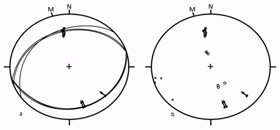
Figure 8.
Regime 8. Lower Hemisphere Equal Area projection of (a) great circles of fault planes and (b) of poles to fault planes (open circles) and of calculated trend and plunge (*) of σ2. Symbols are as in Figure 3.
Because the direction of compression suggested by this pattern of reverse faults is not far from N–S (with an azimuth of compression approximately 160), they may be related to regimes 6–7 through a relative magnitude shift between the intermediate and minimum stress axes. If Regime 8 is added to 6 and 7 the inversion rejects all 4 faults in Regime 8. As in the case of Regimes 2–5, this suggests a common tectonic event involving a stress permutation between σ2 axis and σ3 axes. There is no evidence that Regime 8 resulted from a separate tectonic event.
Event 4 comprising Regimes 6–8 was certainly more recent than the reverse and normal faults of the ductile-brittle transition (compression of Regime 1, and the extension of Regime 2). The contacts of the diabase dikes of Jurassic age are reactivated as strike-slip faults of Regimes 6 and 7 indicating that the faulting and diabase dike intrusion in these regimes occurred 200–146 Ma or later. The NW-SE extension is compatible with the regional extension (based on local NE-SW diabase dike trends, [24]) affecting the study area during the initial opening of the north Atlantic Ocean 200–175 Ma [34], Figure 5.
4.6. Event 5—Regime 9
Regime 9 (Figure 9) corresponds to three strike-slip faults, which trend NW-SE (left-lateral) and WNW-ESE (right-lateral), and hence indicate a roughly NW-SE compression which we label as Event 5. This event is the most recent at the study site. Designation of Regime 9 and calculation of the stress tensor by three fault slips results in a high level of uncertainty.
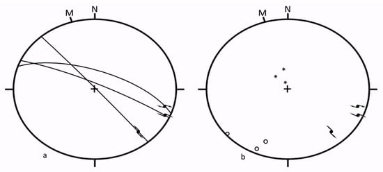
Figure 9.
Regime 9. Lower Hemisphere Equal Area projection of (a) great circles of fault planes and (b) of poles to fault planes (open circles) and of calculated trend and plunge (*) of σ2. Symbols are as in Figure 3.
5. Interpretation
We relate the relative stress tensor in our Events (Table 2) to known tectonic events summarized above in Section 2.
5.1. Event 1—Acadian Compression
This major event is the oldest episode recorded by fault slip at the study site. It was dominated by NW-SE compression (Regime 1) and took place at depth, near the ductile-brittle transition at the or near the end of the Acadian orogeny (390–375 Ma).
5.2. Event 2—Post Acadian Extension
This major event was responsible for widespread normal faulting at a depth, not far from the ductile-brittle transition. Its faults developed under a pure brittle regime at shallower depths, and the faulting was later (375–325 Ma)-than the faults in Event 1. The major NW-SE extension that occurred in this Event parallels the major NW-SE compression of Event 1. This suggests that the extension in Event 2 resulted from the exhumation of metamorphic basement that followed the major compressional phase of Event 1.
5.3. Event 3—Late Alleghenian Compression
The reverse and strike slip faulting of Regimes 4 and 5 are not numerous enough to tightly constrain the corresponding paleo-stresses, and these two Regimes are poorly located in time. They are represented by pure brittle features, and certainly postdate the brittle-ductile deformation, but may not predate Event 4. We tentatively relate these two regimes to the late tectonic evolution of the Alleghenian orogeny (325–260 Ma).
5.4. Event 4—Atlantic Extensional Opening (?)
The strike-slip faulting of Regimes 6 and 7 and the reverse faulting or Regime 8 indicate N–S compression and E-W extension. The presence of a strike-slip fault zone 1–3 m wide suggests that the offsets are relatively large (10–100′s of meters) [35,36,37]. The contacts of the diabase dikes of Jurassic age are reactivated by the strike-slip faults of Regimes 6–7 indicating that the faulting and diabase dike intrusion in these regimes occurred 200–146 Ma or later. The NW-SE extension is compatible with the regional extension (based on local NE-SW diabase dike trends, [24]) affecting the study area during the initial opening of the Atlantic Ocean 200–175 Ma [34], Figure 5.
5.5. Event 5—Recent or Present
This Regime is represented by only a few strike-slip faults with minor offsets. The direction of compression (NW-SE) is consistent with the present state of stress in this region based on earthquake focal mechanisms [38]. We did not observe sheeting joints (sub-horizontal fractures) that can form in response to the unloading of glacial ice [39] over the past 100,000 years.
6. Discussion
This paper illustrates a method to identify distinct regional tectonic events and put them in relative chronological order from fault slip data collected on a few local roadcuts. The data was collected in this case over a period of 10 days. The volume of fault orientation and slip data is relatively small compared to regional field mapping of large scale structures field studies, but by explicitly considering the stress tensors that could have produced the observations, the fault data can be sorted and grouped into Regimes that yield compatible stress tensors that can be further grouped into distinct tectonic Events. In the southwest White Mountain region, the Events identified correspond to known tectonic events based on large scale structures over the last ~400 Ma. The orientation and relative magnitudes of principal stresses producing major regional tectonic deformations can be obtained relatively quickly from a study at one locality.
The conditions for this study were close to ideal because the roadcuts exposed unaltered rocks recently exhumed by the last glaciation. The direct inversion method could potentially be applied using oriented cores from boreholes where there are no outcrops. This paper illustrates how, if the stress tensor can be constrained, the history of overprinted deformation that could have impacted basin resources can be deduced from features on the surfaces of fractures reactivated by sequential tectonic events.
Author Contributions
C.C.B.: field collection of data 50%, writing of manuscript 90%. J.A.: field collection of data 50%, inversion of data and identification of regimes and events 95%, writing of manuscript 10%. All authors have read and agreed to the published version of the manuscript.
Funding
C.C. Barton was supported by the U.S. Geological Survey as part of his employment. J. Angelier was supported by the Universite Pierre et Marie Curie as part of his employment.
Acknowledgments
The authors wish to acknowledge support from the U.S. Geological Survey. J. Angelier was an early key developer of the Direct Inversion Method of Fault-Slip Analysis for unraveling tectonic history to deduce paleo stress orientations and relative magnitudes from surface structures on the faces rock fractures reactivated by sequential tectonic activity. Readers are directed to his many papers on this subject. He was a pleasure to work with in the field. His field notebooks were magnificent and artistically beautiful. His intelligence, enthusiasm, and good company is missed by those who knew and worked with him. Jacques Angelier died in January 2010. The authors thank Tristan Coffey who drafted the figures and tables. The authors thank C. Page Chamberlain and Gautum Mitra who provided early reviews of this manuscript and two anonymous additional reviewers. The authors also thank Lawrence Cathles who provided a thorough edit for this volume
Conflicts of Interest
The authors declare no conflict of interest.
Data Availability
The data collected for each fault listed in tabular form in Appendix A is also available at: http://www.hubbardbrook.org/data/dataset_search.php.
Appendix A. List of Data Collected in This Study
- Explanation to Columns in Table A1
- Column A–Fault Reference Number
- Column B–Fault Strike (azimuth)
- Column C–Fault Dip and Direction
- Column D–Rake of Slip Striations
- Column E–Regime Number/Relative Chronology (1 = oldest, 9 = youngest)
- Certainty (C = certain, P = probable, S = inferred)
- Column F–Fault Location on Interstate 93:
- SBLW = Southbound Lane, West Side of I-93, [10] sheet 2
- SBLE = Southbound Lane, East Side of I-93, [10] sheet 2.
- NBLW = Northbound Lane, East Side of I-93, [10] sheet 2
- NBLE = Northbound Lane, West Side of I-93, [10] sheet 2
- Column G–Fracture Reference Numbers on [10] sheet 2
- Column H–Site location (see Figure 1)
Table A1.
Fault Data Collected and Analyzed in This Study.
Table A1.
Fault Data Collected and Analyzed in This Study.
| A | B | C | D | E | F | G | H |
|---|---|---|---|---|---|---|---|
| 1 | 173 | 77W | 43N | 6C | SBLE | 1 | 1 |
| 2 | 41 | 40E | 45N | 2C 4C | SBLE | 42 | 1 |
| 3 | 32 | 38E | 62N | 2C 4C | SBLE | 42 | 1 |
| 4 | 95 | 64N | 40W | 1C 1C | SBLE | 42A | 1 |
| 5 | 163 | 83W | 40N | 6C | SBLE | 11A | 1 |
| 6 | 163 | 83W | 40N | 1C | SBLE | 11 | 1 |
| 7 | 166 | 85W | 44N | 6C | SBLE | 11A | 1 |
| 8 | 165 | 83W | 38N | 6C | SBLE | 11A | 1 |
| 9 | 159 | 77W | 9S | 7C | SBLE | 19 | 1 |
| 10 | 152 | 88W | 20S | 7C | SBLE | 14B | 1 |
| 11 | 159 | 78W | 17S | 7C | SBLE | 14B′ | 1 |
| 12 | 153 | 89W | 34S | 7C | SBLE | 22 | 1 |
| 13 | 137 | 89W | 41S | 7C | SBLE | 22 | 1 |
| 14 | 153 | 77W | 46S | 7C | SBLE | 22 | 1 |
| 15 | 165 | 84W | 46S | 7C | SBLE | 22′ | 1 |
| 16 | 146 | 81W | 25S | 7C | SBLE | 21 | 1 |
| 17 | 141 | 88W | 43S | 7C | SBLE | 21 | 1 |
| 18 | 139 | 88W | 36S | 7C | SBLE | 20 | 1 |
| 19 | 136 | 77W | 33S | 7C | SBLE | 20 | 1 |
| 20 | 158 | 76W | 24S | 7C | SBLE | 19′ | 1 |
| 21 | 3 | 69W | 31S | 7C | SBLE | unmapped | 1 |
| 22 | 157 | 77W | 23S | 7C | SBLE | 19′ | 1 |
| 23 | 3 | 69W | 31S | 7C | SBLE | unmapped | 1 |
| 24 | 55 | 48N | 52W | 3C | SBLE | unmapped ou 18A | 1 |
| 25 | 61 | 46N | 47W | 3C | SBLE | unmapped ou 18A | 1 |
| 26 | 48 | 77N | 76W | 3C | SBLE | unmapped ou 18A | 1 |
| 27 | 29 | 63W | 73S | 3C | SBLE | 24 | 1 |
| 28 | 28 | 52E | 68S | 1C | SBLE | 25 | 1 |
| 29 | 47 | 87S | 29W | 7C | SBLE | unmapped | 1 |
| 30 | 42 | 88E | 3S | 1C 7C | SBLE | unmapped | 1 |
| 31 | 177 | 42E | 61N | 2C 4C | SBLE | 48 | 1 |
| 32 | 178 | 44E | 21S | 1C 7C | SBLE | 48 | 1 |
| 33 | 178 | 44E | 60N | 2C 4C | SBLE | 48 | 1 |
| 34 | 18 | 48E | 51S | 3C | SBLE | 49 | 1 |
| 35 | 26 | 77E | 25N | 1C 6C | SBLE | 67 | 1 |
| 36 | 26 | 77E | 79S | 2C 3C | SBLE | 67 | 1 |
| 37 | 13 | 51E | 37S | 3C | SBLE | 98? | 1 |
| 38 | 12 | 88W | 12S | 7C | SBLE | unmapped | 1 |
| 39 | 176 | 60E | 46N | 6C | SBLE | unmapped | 1 |
| 40 | 48 | 87N | 7E | 1C 5C | SBLE | 107 | 1 |
| 41 | 48 | 87N | 75E | 2C 3C | SBLE | 107 | 1 |
| 42 | 30 | 87E | 82N | 3C | SBLE | 106 | 1 |
| 43 | 41 | 78E | 17N | 5C | SBLE | 116A proche | 1 |
| 184 | 43 | 80E | 15N | 5C | SBLE | 116A proche | 1 |
| 182 | 28 | 70W | 23S | 7C | SBLE | 116 | 1 |
| 183 | 41 | 75E | 74S | 3C | SBLE | 116 | 1 |
| 44 | 54 | 87N | 29W | 5C | SBLE | 116 | 1 |
| 45 | 32 | 66E | 33S | 5C | SBLE | unmapped | 1 |
| 46 | 30 | 71E | 81N | 3C | SBLE | 123 | 1 |
| 47 | 30 | 71E | 18N | 5C | SBLE | 123 | 1 |
| 48 | 39 | 72E | 83S | 3C | SBLE | unmapped | 1 |
| 49 | 51 | 84S | 72W | 1C 3C | SBLE | 130 | 1 |
| 50 | 18 | 20W | 53N | 2C 1C | SBLE | 138 | 1 |
| 51 | 51 | 84S | 10E | 1C 5C | SBLE | 130 | 1 |
| 52 | 17 | 21W | 53N | 2C 1C | SBLE | 138 | 1 |
| 53 | 50 | 83S | 73W | 3C | SBLE | 130 | 1 |
| 54 | 50 | 83S | 9E | 5C | SBLE | 130 | 1 |
| 55 | 73 | 34S | 63E | 1C | SBLE | unmapped | 1 |
| 56 | 67 | 41S | 66E | 1C | SBLE | 139 | 1 |
| 57 | 59 | 76N | 28E | 5C | SBLE | 146 | 1 |
| 58 | 66 | 63N | 28E | 5C | SBLE | unmapped | 1 |
| 59 | 57 | 76S | 15W | 5C | SBLE | 162 | 1 |
| 60 | 24 | 74E | 12N | 1P 5C | SBLE | 166 | 1 |
| 61 | 24 | 74E | 30N | 2P 7C | SBLE | 166 | 1 |
| 62 | 24 | 74E | 64S | 1P 3C | SBLE | 166 | 1 |
| 63 | 25 | 75E | 30N | 2P 6C | SBLE | 166 | 1 |
| 64 | 47 | 87N | 22E | 6C | SBLW | 66 | 1 |
| 65 | 96 | 89S | 67E | 1C | SBLW | 49 | 1 |
| 66 | 57 | 86S | 37E | 5C | SBLW | 48 | 1 |
| 67 | 17 | 88E | 73S | 3C | SBLE | unmapped | 1 |
| 68 | 25 | 56W | 61S | 2C 1C | SBLW | 25 | 1 |
| 69 | 25 | 56W | 62N | 1C 1C | SBLW | 25 | 1 |
| 70 | 25 | 56W | 16S | 2C 5C | SBLW | 25 | 1 |
| 71 | 25 | 54W | 64N | 1C 1C | SBLW | 25 | 1 |
| 72 | 71 | 33N | 82E | 1C 8C | SBLW | 24 | 1 |
| 73 | 71 | 33N | 42E | 2C 6C | SBLW | 24 | 1 |
| 74 | 52 | 32N | 63E | 8C | SBLW | 24 | 1 |
| 75 | 76 | 22S | 58E | 1C 8C | SBLW | 24 | 1 |
| 76 | 71 | 31N | 82E | 2C 8C | SBLW | 24 | 1 |
| 77 | 78 | 21S | 84E | 8C | SBLW | 24 | 1 |
| 78 | 75 | 23S | 88E | 8C | SBLW | 24 | 1 |
| 79 | 7 | 70E | 62S | 3C | SBLW | unmapped | 1 |
| 80 | 10 | 43E | 76S | 3C | SBL | unreferenced | 1 |
| 81 | 29 | 71W | 24N | 5C | NBLW | 1 | 1 |
| 82 | 37 | 76W | 29N | 5C | NBLW | 1 | 1 |
| 83 | 42 | 74W | 35N | 5C | NBLW | 1 | 1 |
| 84 | 48 | 72N | 12E | 5C | NBLW | 1 | 1 |
| 85 | 142 | 19W | 85S | 4C | NBLW | unmapped | 1 |
| 86 | 68 | 33S | 64E | 3C | NBLW | 9 | 1 |
| 87 | 69 | 35S | 37E | 3C | NBLW | 1 | |
| 88 | 46 | 52S | 63E | 3C | NBLW | 12-11月 | 1 |
| 89 | 52 | 47S | 63E | 3C | NBLW | 12-11月 | 1 |
| 90 | 51 | 38S | 52E | 3C | NBLW | 12 | 1 |
| 91 | 46 | 42S | 84E | 3C | NBLW | 13 | 1 |
| 92 | 45 | 44S | 83E | 3C | NBLW | 13 | 1 |
| 93 | 14 | 20E | 73S | 3C | NBLW | near F29 | 1 |
| 94 | 22 | 25E | 85S | 3C | NBLW | near F29 | 1 |
| 95 | 21 | 33E | 74S | 1C | NBLW | 28 | 1 |
| 96 | 21 | 54E | 72S | 1C | NBLW | 28 | 1 |
| 97 | 58 | 33S | 67E | 1C | NBLW | unmapped | 1 |
| 98 | 46 | 58S | 66E | 3C | NBLW | unmapped | 1 |
| 99 | 41 | 27E | 77N | 1C | NBLW | 35 | 1 |
| 100 | 29 | 50E | 72N | 3C | NBLW | 71 | 1 |
| 101 | 31 | 81E | 18S | 5C | NBLW | 73 | 1 |
| 102 | 67 | 81N | 6E | 7C | NBLW | unmapped | 1 |
| 103 | 38 | 89E | 9S | 7C | NBLW | unmapped | 1 |
| 104 | 24 | 54E | 64S | 3C | NBLW | 79 | 1 |
| 105 | 15 | 30E | 73S | 3C | NBLW | 79 | 1 |
| 106 | 10 | 36E | 68S | 3C | NBLW | 79 | 1 |
| 107 | 29 | 46E | 87S | 3C | NBLW | 80 | 1 |
| 108 | 29 | 48E | 89S | 3C | NBLW | 80 | 1 |
| 135 | 29 | 48E | 88S | 1C | NBLW | 80 | 1 |
| 109 | 110 | 69N | 11E | 9C | NBLW | unmapped | 1 |
| 110 | 139 | 89E | 19S | 9C | NBLW | unmapped | 1 |
| 111 | 20 | 85W | 12N | 5C | NBLW | 1 | |
| 112 | 165 | 57W | 60S | 3C | NBLW | 1 | |
| 113 | 63 | 86N | 1W | 5C | NBLW | 1 | |
| 114 | 21 | 65E | 76N | 3C | NBLW | 86 | 1 |
| 115 | 160 | 83E | 4S | 7C | NBLW | 122? | 1 |
| 116 | 161 | 80E | 14S | 7C | NBLW | 123? | 1 |
| 117 | 150 | 75E | 10S | 7C | NBLW | 123? | 1 |
| 118 | 166 | 84E | 7S | 7C | NBLW | 118 | 1 |
| 119 | 25 | 83E | 2N | 7C | NBLW | unmapped | 1 |
| 120 | 177 | 76E | 2S | 7C | NBLW | unmapped | 1 |
| 121 | 26 | 51E | 64N | 3C | NBLW | unmapped | 1 |
| 122 | 1 | 82E | 2S | 7C | NBLW | 130? | 1 |
| 123 | 170 | 86E | 7S | 7C | NBLW | 133? | 1 |
| 124 | 4 | 82E | 1N | 7C | NBLW | 131? | 1 |
| 125 | 14 | 47E | 79S | 3C | NBLW | unmapped | 1 |
| 126 | 47 | 47S | 33E | 5C | NBLW | 135 | 1 |
| 127 | 179 | 62W | 80N | 3C | NBLW | unmapped | 1 |
| 128 | 1 | 67W | 84N | 3C | NBLW | 151 | 1 |
| 129 | 156 | 77W | 2S | 7C | NBLW | unmapped | 1 |
| 130 | 12 | 69W | 87S | 3C | NBLW | 156 | 1 |
| 131 | 33 | 77W | 3S | 7C | NBLW | 156 | 1 |
| 132 | 7 | 57W | 71S | 3C | NBLW | unmapped | 1 |
| 133 | 13 | 64W | 77N | 3C | NBLW | unmapped | 1 |
| 134 | 8 | 55W | 72S | 3C | NBLW | unmapped | 1 |
| 185 | 155 | 62E | 80S | 3C | NBLW | unmapped | 1 |
| 186 | 28 | 82E | 77S | 1C 3C | NBLW | unmapped | 1 |
| 187 | 28 | 82E | 4N | 2C 7C | NBLW | unmapped | 1 |
| 136 | 32 | 79W | 79N | 3C | NBLE | unmapped | 1 |
| 137 | 34 | 72E | 74N | 3C | NBLE | 36 | 1 |
| 138 | 34 | 85E | 8S | 7C | NBLE | large fault | 1 |
| 139 | 36 | 66E | 2N | 7C | NBLE | large fault | 1 |
| 140 | 174 | 75E | 17N | 7C | NBLE | unmapped | 1 |
| 141 | 176 | 83W | 27N | 7C | NBLE | 46 | 1 |
| 142 | 175 | 88E | 15N | 7C | NBLE | 46 | 1 |
| 143 | 178 | 79E | 2S | 7C | NBLE | 53 | 1 |
| 144 | 30 | 39E | 10N | 2C 7C | NBLE | 51 | 1 |
| 145 | 30 | 39E | 75S | 1C 3C | NBLE | 51 | 1 |
| 146 | 32 | 88W | 6N | 7C | NBLE | 55 | 1 |
| 147 | 41 | 86E | 3S | 7C | NBLE | 64 | 1 |
| 148 | 37 | 82W | 1S | 7C | NBLE | 64 | 1 |
| 149 | 17 | 61E | 83S | 3C | NBLE | 58 | 1 |
| 150 | 35 | 73W | 63S | 3C | NBLE | unmapped | 1 |
| 151 | 114 | 84N | 5E | 9C | NBLE | 68 | 1 |
| 152 | 42 | 85E | 1S | 7C | NBLE | 70 | 1 |
| 153 | 50 | 89S | 7W | 7C | NBLE | 74 | 1 |
| 154 | 35 | 82W | 12S | 7C | NBLE | 74 | 1 |
| 155 | 44 | 88E | 6S | 7C | NBLE | 74 | 1 |
| 156 | 40 | 72W | 11S | 7C | NBLE | 87-89 | 1 |
| 157 | 39 | 81W | 1S | 7C | NBLE | 87-89 | 1 |
| 158 | 29 | 85W | 36N | 7C | NBLE | 87-89 | 1 |
| 159 | 10 | 83W | 14N | 7C | NBLE | 87-89 | 1 |
| 160 | 32 | 80E | 84N | 3C | NBLE | 91 | 1 |
| 161 | 29 | 84E | 28N | 7C | NBLE | 91 | 1 |
| 162 | 46 | 72N | 88E | 3C | NBLE | 98 | 1 |
| 163 | 58 | 68S | 76E | 1C 3C | NBLE | 105 | 1 |
| 164 | 58 | 68S | 22E | 2C 7C | NBLE | 105 | 1 |
| 165 | 35 | 42E | 82N | 3C | NBLE | unmapped | 1 |
| 166 | 19 | 73E | 66S | 1C | NBLE | unmapped | 1 |
| 167 | 22 | 47E | 80N | 3C | NBLE | unmapped | 1 |
| 168 | 52 | 73S | 13E | 7C | NBLE | 111 | 1 |
| 169 | 46 | 89N | 12E | 7C | NBLE | 130? | 1 |
| 170 | 36 | 82E | 34N | 2C 7C | NBLE | 136? | 1 |
| 171 | 36 | 82E | 1C 3C | NBLE | 136? | 1 | |
| 172 | 22 | 49W | 64S | 3C | NBLE | unmapped | 1 |
| 173 | 42 | 53W | 53S | 3C | NBLE | 163? | 1 |
| 174 | 25 | 67W | 52S | 3C | NBLE | 164? | 1 |
| 175 | 44 | 67W | 49S | 3C | NBLE | unmapped | 1 |
| 176 | 16 | 49W | 74N | 3C | NBLE | unmapped | 1 |
| 177 | 36 | 87E | 82S | 1C | NBLE | unmapped | 1 |
| 178 | 23 | 52W | 85N | 3C | NBLE | unmapped | 1 |
| 179 | 23 | 62W | 85S | 3C | NBLE | unmapped | 1 |
| 180 | 26 | 65W | 83S | 3C | NBLE | unmapped | 1 |
| 181 | 15 | 42W | 89N | 3C | NBLE | unmapped | 1 |
| 188 | 35 | 77E | 66N | 3C | NBLE | 2 | |
| 189 | 32 | 74E | 88N | 3C | NBLE | 2 | |
| 190 | 33 | 80E | 66N | 3C | NBLE | 2 | |
| 191 | 36 | 72W | 77N | 3C | NBLE | 2 | |
| 192 | 26 | 83W | 77S | 3C | NBLE | 2 | |
| 193 | 146 | 65E | 72N | 2C | NBLE | 2 | |
| 194 | 106 | 44S | 63W | 1C 2C | NBLE | 2 | |
| 195 | 106 | 44S | 19E | 2C 5C | NBLE | 2 | |
| 196 | 33 | 52E | 65S | 3C | NBLE | 2 | |
| 197 | 133 | 87N | 74W | 2C | NBLE | 2 | |
| 198 | 145 | 65E | 68N | 2C | NBLE | 2 | |
| 199 | 125 | 48S | 77W | 1C 2C | NBLE | 2 | |
| 200 | 125 | 48S | 2E | 2C 5C | NBLE | 2 | |
| 201 | 174 | 51E | 68N | 2C | NBLE | 2 | |
| 202 | 6 | 71W | 86N | 3C | NBLE | 2 | |
| 203 | 159 | 76E | 62N | 2C | NBLE | 2 | |
| 204 | 24 | 57W | 81S | 3C | NBLE | 2 | |
| 205 | 11 | 67W | 82S | 3C | NBLE | 2 | |
| 206 | 148 | 63E | 72N | 2C | NBLE | 2 | |
| 207 | 127 | 87N | 71W | 2C | NBLE | 2 | |
| 208 | 128 | 89N | 68W | 2C | NBLE | 2 |
References
- Angelier, J. Example of informatics applied to structural analysis—Some methods for studying fault tectonics. Revue Geographie Physique Geologie Dynamique 1975, 17, 137–145. [Google Scholar]
- Angelier, J. Tectonic analysis of fault slip data sets. J. Geophys. Res. Solid Earth 1984, 89, 5835–5848. [Google Scholar] [CrossRef]
- Angelier, J. From orientation to magnitudes in paleostress determinations using fault slip data. J. Struct. Geol. 1989, 11, 37–50. [Google Scholar] [CrossRef]
- Angelier, J. Inversion of field data in fault tectonics to obtain the regional stress-III. A new rapid direct inversion method by analytical means. Geophys. J. Int. 1990, 103, 363–376. [Google Scholar] [CrossRef]
- Angelier, J. Analyse chronologique matricielle et succession régionale des événements tectoniques. Comptes Rendus Académie Sci. 1991, 312, 1633–1638. [Google Scholar]
- Angelier, J. Palaeostress Analysis of Small-Scale Brittle Structures. In Continental Deformation; Hancock, P., Ed.; Pergamon Press: Oxford, UK, 1994; pp. 53–100. [Google Scholar]
- Hu, J.C.; Angelier, J. Stress permutations: Three-dimensional distinct element analysis accounts for a common phenomenon in brittle tectonics. J. Geophys. Res. Space Phys. 2004, 109, B09403. [Google Scholar] [CrossRef]
- Hancock, P.L. Brittle Microtectonics: Principles and Practice. J. Struct. Geol. 1985, 7, 437–457. [Google Scholar] [CrossRef]
- Mattauer, M. Les Déformations des Matériaux de l’Écorce Terrestre; Herman: Paris, France, 1973; 493p. [Google Scholar]
- Lawn, B.R. Fracture of Brittle Solids, 2nd ed.; Cambridge University Press: Cambridge, UK, 1993; p. 378. [Google Scholar]
- Riedel, W. Zur mechanik geologischer brucherscheinungen. Centralblatt fur Minerologie. Geol. Paleontol. 1929, 354–368. [Google Scholar]
- Carey, E.; Brunier, B. Analyse théorique et numérique d’un modèle mécanique élémentaire appliqué à l’étude d’une population de failles. Comptes Rendus Académie Sci. 1974, 279, 891–894. [Google Scholar]
- Angelier, J. Inversion of earthquake focal mechanisms to obtain the seismotectonic stress IV-a new method free of choice among nodal planes. Geophys. J. Int. 2002, 150, 588–609. [Google Scholar] [CrossRef]
- Navabpour, P.; Angelier, J.; Barrier, E. Cenozoic post-collisional brittle tectonic history and stress reorientation in the High Zagros Belt (Iran, Fars Province). Tectonophysics 2007, 432, 101–131. [Google Scholar] [CrossRef]
- Bergerat, F.; Angelier, J.; Andreasson, P.G. Evolution of paleostress fields and brittle deformation of the Tornquist Zone in Scania (Sweden) during Permo-Mesozoic and Cenozoic times. Tectonophysics 2007, 444, 93–110. [Google Scholar] [CrossRef]
- Barton, C.C.; Camerlo, R.H.; Bailey, S.W. Bedrock Geologic Map of Hubbard Brook Experimental Forest and Maps of Fractures and Geology in Roadcuts along Interstate I-93, Grafton County, New Hampshire; U.S. Geological Survey Miscellaneous Investigation Series map 1-2562, 2 sheets, 1:12,000; U.S. Geological Survey: Reston, VA, USA, 1997.
- Burton, W.C.; Walsh, G.W.; Armstrong, T.R. Bedrock Geologic Map of the Hubbard Brook Experimental Forest, Grafton County, New Hampshire; U.S. Geological Survey Digital Open File Report 00-45, map, text, and computer files; U.S. Geological Survey: Reston, VA, USA, 2000.
- Hatch, N.L.; Moench, R.H. Bedrock Geologic Map of the Wildernesses and Roadless Areas of the White Mountain National Forest, Coos, Carroll, and Grafton Counties, New Hampshire; Miscellaneous Field Studies map—U.S. Geological Survey, Report: MF-1594-A, 1 sheet, scale 1:125,000; U.S. Geological Survey: Reston, VA, USA, 1984.
- Moke, C.B. The Geology of the Plymouth Quadrangle, New Hampshire; scale 1:62,500; New Hampshire Planning and Development Commission: Concord, NH, USA, 1945; p. 21. [Google Scholar]
- Lyons, J.B.; Bothner, W.A.; Moench, R.H.; Thompson, J.B., Jr. Bedrock Geologic Map of New Hampshire; U.S. Geological Survey State Geologic map, 2 sheets, scales 1:250,000 and 1:500,000; U.S. Geological Survey: Reston, VA, USA, 1997.
- Hatch, N.L., Jr.; Moench, R.H.; Lyons, J.B. Silurian-Lower Devonian stratigraphy of eastern and south-central New Hampshire; extensions from western Maine. Am. J. Sci. 1983, 283, 739–761. [Google Scholar] [CrossRef]
- Robinson, P.; Tucker, R.D.; Bradley, D.C.; Berry, I.V.N.H.; Osberg, P.H. Paleozoic orogens in New England, USA. Gff 1998, 120, 119–148. [Google Scholar] [CrossRef]
- Johnson, C.D.; Dunstan, A.M. Lithology and Fracture Characterization from Drilling Investigations in the Mirror Lake Area: From 1979 Through 1995 in Grafton County, New Hampshire; U.S. Geological Survey Water-Resources Investigations Report 98-4183; U.S. Geological Survey: Reston, VA, USA, 1998; p. 210.
- McHone, J.G. Tectonic and paleostress patterns of Mesozoic intrusions in eastern North America. In Triassic-Jurassic Rifting: Continental Breakup and the Origin of the Atlantic Ocean and Passive Margins, Part B; Manspeizer, W.R., Ed.; Elsevier: Amsterdam, The Netherlands, 1988; pp. 607–619. [Google Scholar]
- Thompson, W.B. History of research on glaciation in the White Mountains, New Hampshire (U.S.A.). Géographie Physique Quaternaire 2002, 53, 7–24. [Google Scholar] [CrossRef][Green Version]
- Tarasov, L.; Dyke, A.S.; Neal, R.M.; Peltier, W.R. A data-calibrated distribution of deglacial chronologies for the North American ice complex from glaciological modeling. Earth Planet. Sci. Lett. 2012, 315, 30–40. [Google Scholar] [CrossRef]
- Fowler, B.K.; Davis, P.T.; Thompson, W.B.; Eusden, J.D.; Dulin, I.T. The Alpine zone and Glacial Cirques of Mount Washington and the Northern Presidential Range, White Mountains, New Hampshire. In Proceedings of the 75th Annual Reunion of the Northeastern Friends of the Pleistocene, Pinkham Notch, NH, USA, 1–3 June 2012; p. 35. [Google Scholar]
- Barton, C.C. Characterizing bedrock fractures in outcrops for studies of ground-water hydrology—An example from Mirror Lake, Grafton County, New Hampshire. In U.S. Geological Survey Toxic Substances Hydrology Program, Proceedings of the Technical Meeting, Colorado Springs, CO, USA, 20–24 September 1993; Morganwalp, D.W., Aronson, D.A., Eds.; U.S. Geological Survey Water-Resources Investigations Report 94-4015; U.S. Geological Survey: Reston, VA, USA, 1996; pp. 81–88. [Google Scholar]
- Daubree, M. Application de la méthode expérimentale à l’étude des déformations et des cassures terrestres. Bulletin Societe Geologique France 1879, 3, 108–141. [Google Scholar]
- Anderson, E.M. The Dynamics of Faulting, 2nd ed.; Oliver & Boyd: Edinburgh, UK, 1942; p. 206. [Google Scholar]
- Bott, M.H.P. The Mechanics of Oblique Slip Faulting. Geol. Mag. 1959, 96, 109–117. [Google Scholar] [CrossRef]
- Wallace, R.E. Geometry of Shearing Stress and Relation to Faulting. J. Geol. 1951, 59, 118–130. [Google Scholar] [CrossRef]
- Dupin, J.M.; Sassi, W.; Angelier, J. Homogeneous stress hypothesis and actual fault slip: A distinct element analysis. J. Struct. Geol. 1993, 15, 1033–1043. [Google Scholar] [CrossRef]
- Faure, S.; Tremblay, A.; Malo, M.; Angelier, J. Paleostress Analysis of Atlantic Coastal Extension in the Quebec Appalachians. J. Geol. 2006, 114, 435–448. [Google Scholar] [CrossRef]
- Cowie, P.A.; Scholz, C.H. Physical explanation for the displacement length relationship of faults using a post-yield fracture- mechanics model. J. Struct. Geol. 1992, 14, 1133–1148. [Google Scholar] [CrossRef]
- Faulkner, D.R.; Mitchell, T.M.; Jensen, E.; Cembrano, J.M. Scaling of fault damage zones with displacement and the implications for fault growth processes. J. Geophys. Res. Space Phys. 2011, 116. [Google Scholar] [CrossRef]
- Scholz, C.H.; Dawers, N.H.; Yu, J.Z.; Anders, M.H.; Cowie, P.A. Fault growth and fault scaling laws: Preliminary results. J. Geophys. Res. Space Phys. 1993, 98, 21951–21961. [Google Scholar] [CrossRef]
- Heidbach, O.; Tingay, M.; Barth, A.; Reinecker, J.; Kurfe, B.D.; Muller, B. World Stress Map, 2nd ed.; 1 sheet; Commission for the Geological map of the World: Paris, France, 2009; Available online: http://dc-app3-14.gfz-potsdam.de/pub/poster/World_Stress_map_Release_2008.pdf (accessed on 31 October 2020).
- Jahns, R.H. Sheet Structure in Granites: Its Origin and use as a Measure of Glacial Erosion in New England. J. Geol. 1943, 51, 71–98. [Google Scholar] [CrossRef]


Publisher’s Note: MDPI stays neutral with regard to jurisdictional claims in published maps and institutional affiliations. |
© 2020 by the authors. Licensee MDPI, Basel, Switzerland. This article is an open access article distributed under the terms and conditions of the Creative Commons Attribution (CC BY) license (http://creativecommons.org/licenses/by/4.0/).