GPU-Accelerated Data-Driven Surrogates for Transient Simulation of Tileable Piezoelectric Microactuators

Abstract

Finite element analysis (FEA) remains the gold standard for simulating piezoelectric microactuators because it resolves coupled electromechanical fields with high fidelity. However, transient FEA becomes prohibitively expensive when thousands of actuators must be simulated. This work presents a data-driven surrogate modeling framework for tileable, PZT-5H microactuators enabling fast, dynamic, and parallel predictions of actuator displacement over multi-step horizons from short displacement history windows, augmented with the corresponding prescribed voltage and traction samples over that same history window. High-fidelity COMSOL simulations are used to generate a dataset aiming to encompass the full operational envelope of our actuator under stochastically sampled and procedurally generated input waveform families. From these families, we construct a supervised learning dataset of time histories, displacement, and applied loads. From this, we train a recurrent sequence-to-sequence neural network that predicts a multi-step open-loop displacement rollout conditioned on the most recent electromechanical history. The resulting model can be leveraged to perform batched inference for millions of actuators on GPU hardware, opening up a wide range of new applications such as reinforcement learning via digital twins, scalable design and simulation for piezoelectric artificial-muscle systems, and accelerated optimization.

1. Introduction

Piezoelectric microactuators enable high-precision motion control at the micro- and nanoscale, appearing across numerous systems including nanopositioning stages for atomic force microscopy (AFM) [1], microfluidic pumps and valves [2], micropositioners, energy harvesters, and precision sensors [3]. Designing such systems typically relies on the finite element method (FEM) to resolve coupled electromechanical fields. While grounded in well-established constitutive models and numerical formulations, transient FEM for fine meshes and extensive time horizons quickly becomes computationally and temporally expensive, scaling even more unfavorably as model complexity grows. In this work, we focus on creating accelerated simulations through surrogate modeling, driven by accurate and traceable transient FEM data.

First proposed in Chigullapalli and Clark (2012), the s-drive (see Figure 1) piezoelectric microactuator architecture exploits lateral deflection to produce extremely large translational deflections [4]. Apart from an s-drive’s ability to yield significant deflection, it is particularly intriguing due to its nestability, yielding designs with multiplicative displacement, stiffness, or rotation based on the number of s-drives used. In Figure 2, the nestability of the s-drive cantilevers is observed. Furthermore, the s-drive exploits the inverse piezoelectric effect to produce in-plane motion under applied voltage, and conversely, generates electric response under mechanical loading via the direct piezoelectric effect. This dual capability makes the architecture particularly attractive for advanced robotics, producing precise motion and simultaneously rich electrical signals that encode external mechanical stimuli. Yet, when scaling microscale actuation to macroscale displacement, s-drive-based architectures often require thousands, if not millions, of actuators, causing computational resource and runtime requirements to combinatorially explode, making traditional methods unfeasible for large-scale design.

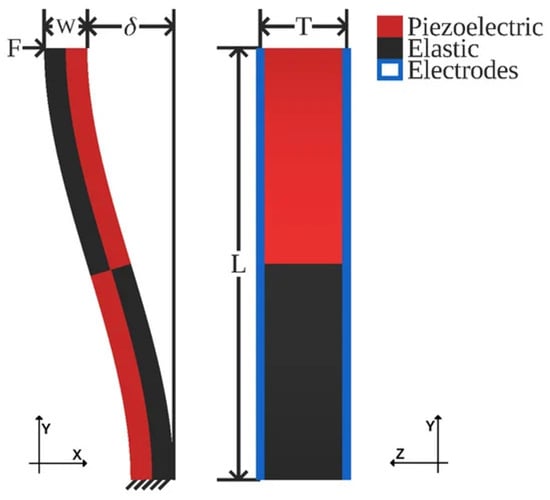
Figure 1. S-drive design from Jones et al. [5].

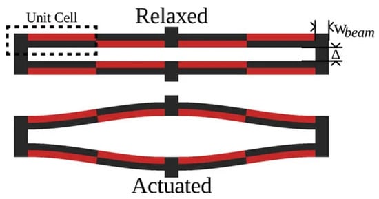
Figure 2. S-drive-based actuator design [5].

Reduced-order models (ROMs) directly address these bottlenecks by approximating the full-order dynamics in a lower-dimensional representation. Classical ROMs like POD-Galerkin, Krylov subspace methods, and balanced truncation can be highly effective for linear or weakly nonlinear systems, yet they often struggle with nonlinear and path-dependent solves without significant augmentation, and are often run concurrently on CPUs. On the other hand, modern neural surrogates can replace expensive PDE solvers with learned dynamics models that are highly optimized for GPUs, exploiting parallelism and millisecond-scale inference.

Much research, both recent and otherwise, has demonstrated the necessity for surrogate modeling. Notably, much promise has been shown in surrogate approaches for time-dependent PDEs and engineering systems, including non-intrusive, high-fidelity predictions of parameterized PDE solutions [6], LSTM-based acceleration in CAE design loops [7], and Gaussian-process surrogates for reliability analysis on complex engineering structures [8]. Furthermore, Meethal et al. (2022) demonstrated a surrogate-FEM middle ground, combining classical FEM with neural networks, creating well-performing and generalizable surrogate models for forward and inverse problems [9].

Along with studies on surrogate modeling in the context of time-dependent PDEs and engineering systems, data-driven approaches have also been explored for the nonlinear and unpredictable behavior of piezoelectric microstructures. Wang et al. (2022) [10] proposed a composite data-driven adaptive control method for piezoelectric linear motors, which learns actuator behaviors from input-output data. The results illustrate how data-driven learning can improve the dynamic and static performances of a piezoelectric linear motor while addressing the unmodeled uncertainties of the system. Similarly, Makarem et al. (2021) [11] showed that resonance-based operation and friction-driven force transfer in piezoelectric ultrasonic motors result in nonlinear effects like creep and hysteresis. In order to address this, a data-driven method was utilized, running iterative feedback tuning of the PID controller parameters as an alternative to model-based control. These works illustrate the effectiveness of data-driven strategies for piezoelectric actuator systems with complex, nonlinear behavior, pointing towards data-driven modeling and surrogate simulation approaches.

Despite these advances, modeling s-drive-based, tileable piezoelectric microactuators under time-varying electromechanical loading has received comparatively limited attention, particularly in the context of scalable microactuator-based systems simulation. In contrast to the aforementioned methods, we seek to develop a highly specialized and lightweight surrogate, suited for simulating many actuators where throughput is more important than single-actuator latency.

In this paper, we introduce a recurrent sequence-to-sequence surrogate that learns actuator dynamics from COMSOL-generated trajectories.

Throughout this work, the surrogate operates in a history-conditioned forecasting setting: given the most recent window of displacements together with the corresponding voltage/traction samples over that same history window, the model predicts the next H displacement futures as an open-loop rollout within the range of electromechanical conditions represented in the training data, enabling fast inference for long-horizon simulations and ensemble predictions.

• Contributions:

• A COMSOL-to-dataset pipeline that produces time-series trajectories spanning diverse voltage/traction waveforms.
• Two lightweight, GPU-optimized recursive sequence-to-sequence surrogate variants that predict displacement rollouts from short history windows.
• Evaluation on a holdout set showing strong fidelity across displacement channels and fast runtimes for a single actuator.
• Evaluation of surrogate runtime scaling; performing batched inference across multiple GPUs, yielding predictions for millions of actuators.

• Limitations of Analytical Modeling

Our surrogate is trained exclusively on finite element data; its accuracy is evaluated relative to the underlying FEA model and does not account for experimental or fabrication-induced discrepancies. Despite this, previous works have demonstrated permissible inaccuracies (≈5%) when comparing empirical actuator displacement to those yielded by FEM for PZT-based s-drives [12]. For increased real-world accuracy, fine-tuning on displacement trajectories generated by numerous fabricated actuators would be required.

2. Methodology

The methodology described in this section defines a data-driven surrogate intended to approximate transient finite element simulations of a single s-drive actuator under prescribed electromechanical loading, rather than a first-principles physical model.

2.1. Actuator Design

Our actuator’s geometry consists of two central shuttles (12 μm × 12 μm × 6 μm), and two structural beams that connect the two s-drive arrays (6 μm × 24 μm × 6 μm). The dimensions of the four s-drive cantilevers are 200 μm × 4 μm × 3 μm, respectively. Since electrode thicknesses for PZT films are relatively thin compared to piezo-region thickness [13,14], it is common practice to neglect electrode geometry and simply apply voltage as a boundary condition [15]. To reduce model complexity, we do not instantiate electrode geometry; we simply apply voltages as checkerboarded boundary conditions on the $\pm z$ faces of the s-drives.

We instantiate our s-drive-based actuator in COMSOL Multiphysics 5.5, defining boundary conditions to excite coupled electromechanical dynamics while enabling consistent measurements of free-shuttle displacement:

1.

Fixed constraint: the exterior face of the fixed shuttle on the $xz$-plane is clamped.

2.

Traction + Displacement Probe: the opposing shuttle’s exterior face is subjected to time-varying traction load, and its displacement is recorded via a boundary probe during solves.

3.

Voltage Terminals: a checkerboarded terminal pattern applies voltage on the top electrodes ($+z$), and all bottom ($-z$) surfaces are grounded.

See Figure 3 and Figure 4 for visualizations of boundary conditions and domain modes.

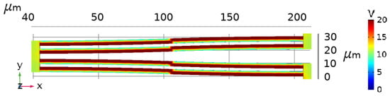
Figure 3. Checkerboarded electrical potential of the top of an actuator half.

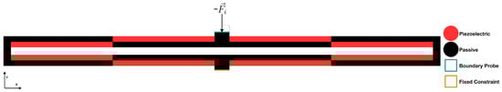
Figure 4. Our PZT-5H Microactuator. Here $\overrightarrow{F_i}$ is the traction we apply to the free-shuttle boundary at simulation step i. We define the boundary probe and fixed constraint as blue and orange, respectively. The actuator spans the bounding box [424 μm, 28 μm, 6 μm].

2.2. Material Selection

Prior work has validated s-drive actuator configurations in PZT-based devices via simulation, fabrication, and empirical tests [12]. We select PZT-5H because (i) its demonstrated effectiveness for s-drive actuation, (ii) PZT-based ceramics have high piezoelectric coefficients and moderate coercive fields reported as ≈585 pC N⁻¹ [16] and 14.9 kV cm⁻¹ for thin films [17], and (iii) as an upper-bound, aggressive-loading regime test case for our surrogate. Within the domain of ceramic piezoelectric materials, Potassium Sodium Niobate (KNN) based compositions have received interest due to their significant experimental $d_{33}$ values ranging from 75.1 to 610 pC N⁻¹ [18,19], moderate coercive fields (11.8–18.1 kV cm⁻¹ [20]), and non-toxicity; a large drawback for PZT ceramics.

Outside of ceramics, many biocompatible alternatives like PVDF and PVDF-TrFe have become particularly intriguing in recent years. In particular, PVDF has been widely explored due to its mechanical strength, chemical inertness, and transparency under certain conditions. With experimental piezoelectric coefficients ranging from $d_{33}$ = 13–35 pC N⁻¹, 24–39 pC N⁻¹ [21]. While relative to ceramics, PVDF may often have lower observed $d_{33}$, but often exhibits very high coercive fields: 200–600 kV cm⁻¹ [22], 1146–1418 kV cm⁻¹ [23], which makes polarization switching more difficult.

For the s-drive, we are primarily interested in higher $d_{31}$ values, which measure the stress produced orthogonally to the polarization axis. Unfortunately, $d_{31}$ is often much harder to measure experimentally; therefore, $d_{33}$ is more commonly used as a metric for deflection. Despite this, they have the following empirical relationship [24]:

$$d_{33}\approx -2.5 d_{31}.$$

(1)

We use COMSOL’s predefined standard linear piezoelectric constitutive model for PZT-5H. Importantly, all material properties are used solely within the finite element simulations that generate training data and are not explicitly enforced within the surrogate model.

2.3. Input Waveform Generation

To elicit a wide range of dynamic responses, we generate excitation waveforms in two stages: (i) 2500 ms of randomly sampled voltage [0–20] V and traction $[-0.14,0.14]$ MPa sampled at $0.1$ ms timesteps and (ii) 2500 ms of all permutations of the following families sampled at $0.15$ ms:

• Voltage waveforms (11 families): pseudorandom binary sequences (PRBS); square-pulse trains with random pulse widths; multi-sine signals (sum of five sinusoids with random frequencies and phases); logarithmic-frequency chirps; triangular waves with random frequency; sawtooth waves with random frequency; random telegraph (two-state) processes; sparse impulse trains (short high-amplitude pulses); hold-then-step waveforms; amplitude-modulated sine waves and colored noise (white noise filtered by a moving-average filter).
• Force waveforms (12 families): pure sinusoidal waves with random frequency; linear ramps (increasing or decreasing); linear-frequency chirps; logarithmic-frequency chirps; piecewise-linear interpolations between randomly sampled anchor points; multi-sine signals (sum of five sinusoids); triangular waves with random frequency; sawtooth waves with random frequency; sparse impulse trains; hold-then-step waveforms; amplitude-modulated sine waves and colored noise.

From these discrete regimes, we interpolate them in COMSOL to prevent discontinuity and highly nonlinear impulses.

2.4. Simulation Hyperparameters

Because the stochastic waveform generation produces widely varying stiffness and excitation time scales, different solver parameters were fixed for each waveform sampling method across all four transient runs:

1.

Gaussian Noise (0–2500 ms),

• Time-Stepping Method: Backward Differentiation Formula (BDF) order 2;
• Relative Tolerance: $1\times {10}^{-5}$;
• Nonlinear Method: Constant (Newton);
• Nonlinear Method Maximum Iterations: 65;

2.

Waveform Family Combinations (2500–5000 ms)

• Time-Stepping Method: Backward Differentiation Formula (BDF) order 1;
• Relative Tolerance: $1\times {10}^{-4}$;
• Nonlinear Method: Constant (Newton);
• Nonlinear Method Maximum Iterations: 20;

For all runs, geometric nonlinearity was enabled to capture large-deformation kinematics (piezoelectric constitutive laws remain linear), Jacobians were updated on every iteration; we used tolerance as our termination technique, and the solution as the criterion.

The mesh is physics-controlled with a normal element size. COMSOL’s meshing procedure selected maximum element size 42.4 μm, minimum element size 7.63 μm, maximum element growth rate $1.5$, curvature factor $0.6$, and resolution of narrow regions $0.5$ as parameters. The resulting mesh consisted of 3881 domain elements, 3726 boundary elements, and 1654 edge elements, yielding 34932 degrees of freedom.

2.5. Transient FEA Simulations and Data Collection

During transient solves, interpolation functions provide voltage inputs to terminals and traction inputs to the free-shuttle boundary, respectively. The interpolated traction is applied normally to the main face of the free shuttle, perturbing displacement in response to external mechanical stimuli. Then, the interpolated voltage is applied to the actuator’s terminals. These interpolated inputs span a large portion of the actuator’s operational envelope, giving the surrogate robust and diverse data. Here, the operational envelope refers to the range of voltage and traction inputs defined by the procedurally generated waveform families and bounds used in the finite element simulations, rather than the full space of physically realizable operating conditions. From our completed solves, we extract our boundary probe’s displacement components $(u,v,w)$ and the interpolated load values at $0.01$$\mathrm{m}\mathrm{s}$ increments. Across four simulations, this yields ≈ 500,000 time-indexed samples spanning the bulk of the actuator’s operational envelope.

2.6. Electromechanical Bounds

Piezoelectric ceramics such as PZT-5H are mechanically brittle and susceptible to fracture, depolarization, and dielectric breakdown when subjected to excessive electromechanical loading [25]. Consequently, defining conservative yet sufficiently rich excitation bounds is critical both for ensuring numerical stability during finite element simulations and for characterizing the operational envelope represented in the surrogate’s training data.

To probe the upper limits of mechanical stress within our modeled actuator, we perform an extreme-load FEA run in which the terminal voltage is fixed at 20 V and the external traction is set to 0.14 MPa, corresponding to the maximum values used during data generation. These values are intentionally aggressive and are not intended to represent nominal operating conditions, but rather to stress-test the actuator and expand the surrogate’s exposure to high-response, nonlinear regimes.

Material failure thresholds for PZT-5H depend strongly on fabrication quality, loading rate, and stress state; however, fracture is commonly reported to initiate in the range of 30–50 MPa [25,26]. From the simulation, we measure actuator domain maximums and averages for the first principal stress as 555.77 MPa and 12.623 MPa, respectively. For completeness, the corresponding Von Mises maximum and average are reported: 378.08 MPa, 22.317 MPa. These metrics are not intended to represent physically realizable operation, but simply as context for our simulation bounds.

It is important to emphasize that Von Mises stress is not a reliable fracture criterion for brittle piezoelectric ceramics, whose failure is largely dominated by crack initiation, tensile stress concentration, and depolarization effects rather than plastic yielding. Both stress variants are reported strictly as conservative indicators of mechanical load intensity rather than definitive predictors of material failure. Accurately determining fracture limits requires empirical testing under representative loading conditions, which is beyond the scope of this work.

These results indicate that the excitation bounds used during data generation substantially exceed the mechanically feasible operating range for real PZT-5H devices. This design choice is deliberate: the surrogate is trained on a numerical envelope that is broader than the physically admissible one, allowing reliable interpolation within feasible regimes while retaining extrapolative capability near edge cases. In deployment, feasible actuation can be enforced by clamping the applied voltage and traction inputs before inference.

In addition to mechanical stress limits, electrical breakdown and depolarization impose critical constraints on feasible actuator operation. For PZT-5H, experimentally reported coercive field strengths typically lie in the range of 8.0–14.9 kV cm⁻¹ [17]. Across the sweep, we monitor the maximum and mean electrical field norm over the actuator domains. We observe that the maximum electric field norm reaches 14.976 kV cm⁻¹ and the mean at 4.6228 kV cm⁻¹ with an applied voltage of 1.5873 V. At the upper bound of applied voltage (20 V), the field norm increases substantially to a maximum of 188.33 kV cm⁻¹ and a mean of 58.427 kV cm⁻¹. Thus, these high-field cases should be interpreted as numerical stress tests rather than physically faithful switching behavior, since ferroelectric hysteresis is not modeled. These results indicate our chosen bounds expand the numerical operating envelope beyond physically feasible regimes, thereby enlarging the surrogate’s training distribution.

Importantly, coercive-field thresholds can vary with experimental conditions, including temperature [16], loading/sampling frequency, and waveform duration. Therefore, although 20 V is likely extreme for ordinary use in this geometry, retaining such high-voltage cases in the dataset enables stress-testing for the surrogate’s ability to handle nonlinearity, more diverse data, and out-of-distribution evaluation of the surrogate under aggressive electrical loading. In deployment, a physically admissible operation can be enforced by clamping the applied voltage such that the resulting electric field remains below an experimentally validated coercive-field threshold for the fabricated device and operating conditions.

2.7. History Length via Ring-Down Analysis

In addition to defining electromechanical bounds, selecting an appropriate history length is critical to ensure the surrogate has adequate temporal context to capture the transient actuator behavior while avoiding unnecessary memory and computational overhead from excessively long windows. To inform our choice, we empirically estimate the actuator’s mechanical response time via a ring-down analysis.

We first perform stationary FEA with prescribed displacement applied to the free-shuttles exterior face in the $+y$ direction. We induce two initial conditions: (i) a displacement of 3.278 μm, corresponding to the mean v-channel displacement observed across all transient FEA runs, and (ii) a displacement of 10.17 μm, corresponding to the maximum observed displacement. Using the stationary solution as the initial condition, we run a transient FEA with all input boundary conditions disabled, allowing the actuator to freely reach equilibrium.

The resulting v-channel displacement trajectories, as displayed in Figure 5, characterize the actuator’s natural settling behavior following an abrupt halt in excitation. For the mean-displacement case, the in-plane displacement decays to near zero within approximately 0.3 ms, corresponding to 30 steps. In the extreme case initialized at the maximum displacement, the actuator settles within approximately 0.4 ms, corresponding to 40 timesteps. In both scenarios, the response exhibits an oscillatory exponential decay characteristic of lightly damped mechanical systems.

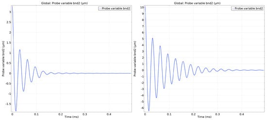
Figure 5. Y-channel displacement vs Time: compares starting displacements at the mean (left) and max (right) measured during data-collection FEA runs.

These results provide a numerically grounded estimate of the required temporal memory to accurately describe the actuator’s state trajectory. While waveforms that push behavior outside of the surrogate’s history window likely exist, our model is trained on diverse data, including many loading conditions and nonlinear transients, enabling it to approximate the system dynamics rather than simply memorizing small input-output pairs.

Based on our analysis, we select a history length of $L=32$ (corresponding to 0.32 ms of FEA simulation), closely matching the observed ringdown time for typical operating conditions. More exhaustive hyperparameter search over history length would incur significant training costs and is unlikely to yield substantial improvements given the scale of our architecture. Therefore, anchoring history length to the actuator’s numerically observed settling time provides a practical and physically interpretable design choice.

2.8. Data Preprocessing

The raw dataset is exported from COMSOL for each transient simulation. Each simulation produces three displacement channels per timestep, denoted as $u\left(t\right),v\left(t\right)$ and $w\left(t\right)$, corresponding to the $x,y$ and z displacement of the probe-surface. Furthermore, the simulation provides two interpolated electromechanical load function tables, representing the voltage load $\left(\mathrm{int}1\right(t\left)\right)$ and external traction applied to the actuator during the transient solve $\left(\mathrm{int}2\right(t\left)\right)$ for each timestep. After parsing the exported COMSOL data, we construct the displacement matrix

$$y\left(t\right)=[u\left(t\right),v\left(t\right),w\left(t\right)]\in {\mathbb{R}}^3,$$

(2)

and our feature vector, which appends the interpolation table

$$x\left(t\right)=[u\left(t\right),v\left(t\right),w\left(t\right),\mathrm{int}1\left(t\right),\mathrm{int}2\left(t\right)]\in {\mathbb{R}}^5.$$

(3)

2.8.1. Training and Validation Splitting

From our FEA data, we chunk transients into non-overlapping sequences of actuator displacement and interpolated loads. Each sequence is then randomly split into our training and validation sets (9:1 split). These held-out waveform families are used for validation to assess generalization across unseen excitation regimes. The resulting shapes for our training and validation sets are as follows:

• $X_{train}$: (455453, 32, 5),
• $Y_{train}$: (455453, 100, 3),
• $X_{val}$: (41405, 32, 5),
• $Y_{val}$: (41405, 100, 3).

2.8.2. Sliding-Window Sequence Generation

Early prototypes mapped voltage-force and displacement histories to the displacement tuple at the next timestep. Despite simplicity, this method incurs longer runtimes as often larger “strides” can be taken without excessive error. To enable stride mechanisms, we train a multi-step surrogate that maps a short history of observed electromechanical states to a future displacement trajectory. Let L denote the encoder history length and H denote the prediction horizon. Our current training script fixes these to

$$L=32,H=100.$$

(4)

The prediction horizon H is chosen to balance computational efficiency, numerical stability, and practical rollout length. With a timestep of 0.01 ms, $H=100$ corresponds to a 1 ms open-loop prediction window, which is long relative to the actuator’s v-channel settling time (≈0.3–0.4 ms) yet short enough to avoid rapid error accumulation inherent to autoregressive forecasting.

We begin by forming at each timestep t, a feature vector containing u, v and w displacement and the two interpolated voltage and traction functions $\mathrm{int}1\left(t\right)$, and $\mathrm{int}2\left(t\right)$:

$$x\left(t\right)=\left[u\left(t\right),v\left(t\right),w\left(t\right),\mathrm{int}1\left(t\right),\mathrm{int}2\left(t\right)\right]\in {\mathbb{R}}^5,$$

(5)

and we define our displacement target vector

$$y\left(t\right)=\left[u\left(t\right),v\left(t\right),w\left(t\right)\right]\in {\mathbb{R}}^3.$$

(6)

A single supervised sample is constructed from a sliding window that uses the past L feature vectors to predict the next H displacement vectors:

$$X_i=\left[x\left(i\right),x(i+1),\dots ,x(i+L-1)\right]\in {\mathbb{R}}^{L\times 5},$$

(7)

$$Y_i=\left[y(i+L),y(i+L+1),\dots ,y(i+L+H-1)\right]\in {\mathbb{R}}^{H\times 3}.$$

(8)

Unlike a naive construction over a single trajectory, our script concatenates multiple simulation segments and enforces that each window remains within a predefined time chunk to minimize leakage across the train/validation split. Concretely, with window length $W=L+H$, we enumerate all candidate start indices $i\in \{0,\dots ,N-W\}$ and retain only those for which the endpoints i and $i+W-1$ lie in the same chunk. Let $\mathcal{I}$ denote this set of valid starts; the dataset size is given by $M=\left|\mathcal{I}\right|$, yielding input tensors of shape $(M,L,5)$ and targets of shape $(M,H,3)$. During preprocessing, inputs are standardized using a mean and standard deviation over the training inputs. To analyze how output standardization affects model performance, we train two models, one using global standardization and the other channel-wise standardization.

During the rollout, the surrogate is evaluated in a history-conditioned forecasting setting: the encoder receives the most recent L samples of $[u,v,w,\mathrm{int}1,\mathrm{int}2]$, while the decoder is driven by displacement (initialized with a zeroed start token and then fed its own predictions).

2.8.3. Feature Standardization

Let $X_{\mathrm{train}}\in {\mathbb{R}}^{M_{\mathrm{train}}\times L\times 5}$ denote the collection of all training windows. To stabilize optimization and prevent single-channel domination of the gradient, all five input features are standardized using mean and standard deviation under global or channel-wise context. For the channel-wise variant, we compute the statistics aggregated jointly over samples and timesteps:

$${\mu }_c={\displaystyle \frac{1}{M_{\mathrm{train}}·L}}\sum _{i=1}^{M_{\mathrm{train}}}\sum _{t=1}^L{X}_{\mathrm{train}}[i,t,c],$$

(9)

$${\sigma }_c=\sqrt{{\displaystyle \frac{1}{M_{\mathrm{train}}·L}}\sum _{i=1}^{M_{\mathrm{train}}}\sum _{t=1}^L{\left(X_{\mathrm{train}}[i,t,c]-{\mu }_c\right)}^{\odot 2}}+ϵ,$$

(10)

with $ϵ={10}^{-6}$ in our implementation. Each training and validation window is then standardized using these same training statistics:

$${\tilde{X}}_i={\displaystyle \frac{X_i-{\mu }_c}{{\sigma }_c}}.$$

(11)

When standardization is applied using global statistics, channels with small physical variance are weighted equally during training and may exhibit large relative error or low $R^2$ despite having small absolute displacement errors.

2.9. Surrogate Model Architecture

The goal is to learn a fast surrogate for the actuator’s transient response conditioned on a recent history of electromechanical states. Contrary to learning a single future state, we predict a future displacement trajectory. This is crucial for efficient rollouts on numerous actuators because predicting H steps at once amortizes the model’s overhead. Given our standardized history window ${\tilde{X}}_i\in {\mathbb{R}}^{L\times 5}$, our sequence to sequence surrogate produces

$${\hat{Y}}_i=f_{\theta }\left({\tilde{X}}_i\right)\in {\mathbb{R}}^{H\times 3},$$

(12)

where each row $\hat{y}\left(t\right)=[\hat{u}\left(t\right),\hat{v}\left(t\right),\hat{w}\left(t\right)]$ is a predicted displacement vector. Our lightweight implementation is well-suited for massive parallel instantiation on GPU hardware.

Our model uses Gated Recurrent Unit (GRU) layers to capture temporal dependencies. Introduced in 2014 by Kyunghyun Cho, the GRU architecture uses update and reset gates to control information flow with comparatively few parameters [27].

• a 2-layer GRU encoder that compresses the L-step input history into a stacked hidden state;
• a 2-layer GRU decoder that autoregressively generates H future displacement vectors conditioned on the encoder’s hidden state;
• and finally, a linear projection that maps the decoder hidden vectors to displacement outputs.

We set the hidden size to 64, and the decoder input dimension is fixed to the output dimension 3.

Among sequence modeling architectures, the Long Short-Term Memory network [28] has a long and successful history of accurate predictions on various tasks. Recently, however, the GRU architecture has proven itself as a worthy competitor, achieving similar and often better performance despite having fewer parameters and lower per-step computational cost [28]. Apart from LSTMs, the Transformer architecture can consistently outperform these architectures for complex tasks like Natural Language Processing (NLP) [29], Protein Folding [30], and Robotic control through NLP and vision [31]. Despite their strong long-range modeling capabilities, GRUs offer more favorable computational requirements and likely similar performance given the short history length and low-dimensional outputs. Furthermore, we report runtime complexities for various other reduced-order modeling architectures in Table 1 for relative differences in scaling. Similar to the LSTM and PINN (under a fixed output field) models, the GRU architecture scales with parameter count $O\left(n_O\right)$ under-offline conditions. If the model is trained, however, for each timestep the runtime scales linearly with respect to actuator count $O\left(1\right)$.

Table 1. Qualitative comparison of ROM methods demonstrating their relation to governing equations, online complexity (for a single actuator), ability to generalize to unseen data, limitations, and common applications. The table taxonomy is as follows: L: number of layers, h: hidden units per layer, d: input feature dimension, $n_x$: number of query points, $n_O$: trainable parameter count, P: number of polynomial terms, M: inducing points, r: reduced-order-model state dimension.

Method	Governing Equations	Online Runtime Complexity	Generalization	Limitations	Examples and Applications
Long Short-Term Memory Networks (LSTMs)	No; data-driven, non-intrusive	$O\left(Lh\right(h+d\left)\right)$; $O\left(1\right)$ (fixed architecture)	Moderate; typically strong within training envelope	Requires extensive and diverse data; training cost	Fluid Dynamics [32,33,34]; Aircraft landing load simulations [35]
Physics-Informed Neural Networks (PINNs)	No; residuals only needed for training	$O\left(n_x{n}_O\right)$; $O\left(n_x\right)$ (fixed architecture)	Strong; physics residual helps with unseen inputs, typically strong within the operational envelope of the training data	Training cost; retraining per problem	Non-Intrusive ROM of parameterized dynamic systems [36]
Polynomial Chaos Expansion (PCE)	No; statistical basis expansion	$O\left(P\right)$; $O\left(1\right)$ (fixed architecture)	Moderate; weak outside design/ parameter space, stronger within	Curse of dimensionality	Dynamic analysis of structures with uncertainties [37]
Gaussian Process Regression (GPR)	No; nonparametric regression on data	≈$\theta$(M) (Sparse Variational GP) [38]	Moderate; Strong in-range, extrapolation trends to the kernel’s mean	Poor scaling with dataset size, curse of dimensionality, kernel sensitivity	ROM of geometrically nonlinear structures [39]
Proper Orthogonal Decomposition (POD-Galerkin)	Yes; projection onto basis	$O\left(r^3\right)$ (Implicit); $O\left(r^2\right)$ (Explicit)	Weak; limited to snapshot manifold, otherwise typically moderate-strong	Poor for highly nonlinear problems (without augmentation)	Microstructure modeling [40]; Blood-flow modeling [41]
Krylov Subspace Methods	Yes; projection of governing equations	$O\left(r^3\right)$ (Implicit); $O\left(r^2\right)$ (Explicit)	Moderate; typically strong for linear systems but weak under nonlinearity	Requires full system matrices;	Nodal analysis for MEMS simulations [42]
Balanced Truncation	Yes; needs full state-space matrices	$O\left(r^3\right)$ (Implicit); $O\left(r^2\right)$ (Explicit)	Typically Moderate	Can struggle with nonlinear dynamics (without augmentation)	Biological oscillator simulations [43]

2.9.1. Dropout and Regularization

Three distinct regularization mechanisms appear in the model definition: (i) input dropout applied to encoder inputs with probability $0.05$; (ii) recurrent-layer dropout internal to PyTorch 2.5.1’s stacked GRU layers with probability $0.1$ between layers and (iii) dropout applied to decoder outputs before projection with probability $0.1$. During training, we also inject Gaussian noise into the standardized input windows.

2.9.2. GRU Encoder

Let $\tilde{X}=[{\tilde{x}}_1,\dots ,{\tilde{x}}_L]$ denote the standardized encoder input sequence, where ${\tilde{x}}_t\in {\mathbb{R}}^5$. We first apply feature dropout to the encoder inputs

$${\overline{x}}_t=\mathrm{Dropout}({\tilde{x}}_t;p_{in}),$$

(13)

and then apply additive Gaussian noise to the standardized windows with standard deviation ${\sigma }_{\mathrm{aug}}=0.005$:

$${\overline{x}}_t\leftarrow {\overline{x}}_t+{\eta }_t,{\eta }_t\sim \mathcal{N}(0,{\sigma }_{aug}^{2}I).$$

(14)

The encoder stacks two GRU layers. For completeness, the GRU updates at a time t for a single layer are

$$\begin{gathered} z_t=\sigma (W_z{\overline{x}}_t+U_z{h}_{t-1}+b_z),r_t=\sigma (W_r{\overline{x}}_t+U_r{h}_{t-1}+b_r), \\ {\tilde{h}}_t=\tanh (W_h{\overline{x}}_t+U_h(r_t\odot h_{t-1})+b_h),h_t=(1-z_t)\odot h_{t-1}+z_t\odot {\tilde{h}}_t. \end{gathered}$$

(15)

In our stacked architecture, the input to layer ℓ is the hidden sequence produced by ℓ − 1. The encoder returns the final hidden state for all layers,

$$H_L^{enc}=[h_L^{\left(1\right)};h_L^{\left(2\right)}]\in {\mathbb{R}}^{K\times d_h},$$

(16)

which is used to initialize the decoder hidden state.

2.9.3. GRU Decoder

The decoder is a stacked GRU with the same number of layers and hidden sizes as the encoder. Unlike the encoder, the decoder input at each step is a predicted displacement vector in ${\mathbb{R}}^3$. The model uses a fixed start of sequence token equal to the zero displacement vector

$$d_0=0\in {\mathbb{R}}^3.$$

(17)

Conditioned on the encoder hidden state, the decoder generates a rollout autoregressively for $t=1,\dots ,H$:

$$(o_t,H_t)={\mathrm{GRU}}_{dec}(d_{t-1},H_{t-1}),H_0=H_L^{enc},$$

(18)

where $o_t\in {\mathbb{R}}^{d_h}$ is the decoder output. Before mapping to displacements, dropout is applied to $o_t$:

$${\overline{o}}_t=\mathrm{Dropout}(o_t;p_{dec}),$$

(19)

and the projection

$${\hat{y}}_t=W_{proj}{\overline{o}}_t+b_{proj}\in {\mathbb{R}}^3,$$

(20)

yields our displacement prediction ${\hat{y}}_t$. Then, finally, the decoder input is set to its own prediction:

$$d_t\leftarrow {\hat{y}}_t.$$

(21)

Stacking the predictions yields $\hat{Y}=[{\hat{y}}_1,\dots ,{\hat{y}}_H]\in {\mathbb{R}}^{H\times 3}$.

2.9.4. Loss Function and Optimization

The mean-squared error over all horizon steps and the displacement channels’ loss function

$$\mathcal{L}\left(\theta \right)={\displaystyle \frac{1}{BHC}}\sum _{i=1}^B\sum _{t=1}^H\sum _{c=1}^C{({\hat{y}}_{i,t,c}-y_{i,t,c})}^2,C=3,$$

(22)

encourages the model to minimize the difference between displacement channels from its prediction and our training set. Here, B is the training batch size, $H:$ horizon length, and c is the displacement channel index.

2.10. Training Hyperparameters

We train the surrogate using the Adam optimizer [44] with learning rate $3\times {10}^{-4}$ and minimize the horizon-averaged MSE in Equation (22) with $B=256$. Training uses automatic mixed precision (AMP) with gradient scaling, global-norm gradient clipping ($\left|\right|\nabla \left|\right|<1.0$), and additive Gaussian noise applied to inputs with standard deviation $\sigma =0.005$ to standardized input windows. A ReduceLROnPlateau scheduler monitors validation loss and decays the learning rate by a factor of $0.5$ after five epochs without improvement, with a learning rate floor of ${10}^{-6}$. Training is terminated after 256 epochs, retaining the checkpoint with the lowest validation loss under a fixed random seed.

3. Results

3.1. Surrogate Accuracy

All results in this section evaluate surrogate predictions relative to held-out finite element simulations and are intended to assess fidelity and computational efficiency with respect to transient FEA. No experimental data are collected; all comparisons are relative to numerical methods. Both training and validation loss curves can be observed in Figure 6.

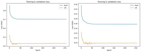
Figure 6. Loss curves for channel-wise norm (left), and global norm (right) variant surrogate models.

3.1.1. Globally Standardized Surrogate

The surrogate under globally normalized input conditioning produces the lowest loss at epoch 32: $\left(0.193\right)$. In particular, to the global variant, we see moderate performance for the v and w channels for the full 100 step rollout: $R^2\left(v\right)=0.6611, R^2\left(w\right)=0.664$. For the w channel, we report MSE as our primary metric as $R^2$ is not descriptive for such low magnitude displacements

$$\mathrm{MSE}\left(u\right)=1.4\times {10}^{-5}.$$

Further results are displayed in Table 2. Because s-drive actuation is designed to produce large in-plane displacement, performance in the v direction is the primary engineering metric of interest, while u and w displacements are secondary and remain near zero under normal operation as seen in Table 3. To correct out-of-plane displacement inaccuracies, we introduce another surrogate under channel-wise, input standardized conditions, reducing v-channel gradient domination.

Table 2. $R^2$ and $MSE$(μm²) with respect to h for the globally standardized surrogate for all displacement channels.

h	${\mathit{R}}^2\left(\mathit{v}\right)$	$\mathbf{MSE}\left(\mathit{u}\right)$	$\mathbf{MSE}\left(\mathit{w}\right)$
1	0.9926	$4.6\times {10}^{-5}$	$3.1\times {10}^{-5}$
2	0.9940	$3.8\times {10}^{-5}$	$2.5\times {10}^{-5}$
4	0.9910	$2.8\times {10}^{-5}$	$2.2\times {10}^{-5}$
8	0.9770	$2.2\times {10}^{-5}$	$2.0\times {10}^{-5}$
16	0.9012	$1.7\times {10}^{-5}$	$1.9\times {10}^{-5}$
32	0.6944	$1.4\times {10}^{-5}$	$2.0\times {10}^{-5}$
64	0.5670	$1.1\times {10}^{-5}$	$2.9\times {10}^{-5}$
100	0.4501	$8.0\times {10}^{-6}$	$4.3\times {10}^{-5}$

Table 3. COMSOL FEA free-shuttle boundary displacement data.

Channel	Min	Max	Mean
u	$-1.491\times {10}^{-3}$ μm	$1.266\times {10}^{-3}$ μm	$-2.032\times {10}^{-4}$ μm
v	$-3.496$ μm	$10.17$ μm	$3.345$ μm
w	$-1.256\times {10}^{-1}$ μm	$1.063\times {10}^{-1}$ μm	$1.148\times {10}^{-4}$ μm

Apart from evaluation on full 100 step rollouts, we can specify a stride length h: “how much we shift the window”. Concretely, this means that successive windows start at indices $i, i+h, i+2h$. For the global-norm conditioned surrogate, $R^2$ for the v-channel displacement generally increases with decreasing stride, reaching a maximum of

$$\underset{h\in \Omega }{\max }{R}^2(v;h)=0.994,$$

(23)

attained at $h=2$, where $\Omega =\{1,2,4,8,16,32,64,100\}$ is the set of stride lengths we evaluate accuracy for. Also see Figure 7 for visualization.

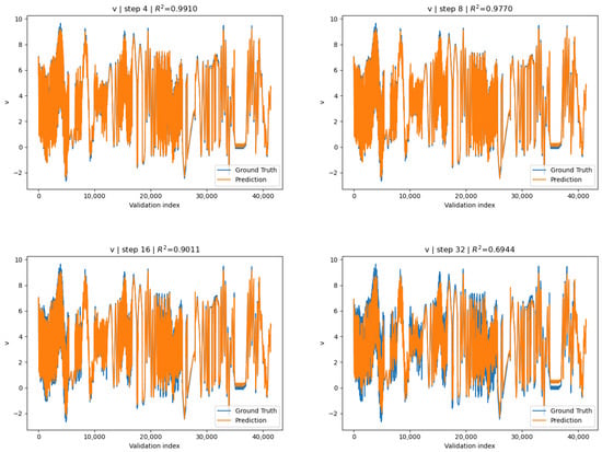
Figure 7. Globally standardized surrogate predictions for the v-direction displacement compared with COMSOL ground truth for stride lengths $h\in \{4,8,16,32\}$. Each panel corresponds to one constant stride-length. Displacements are reported in μm.

3.1.2. Channel-Wise Standardized Surrogate

After training, epoch 13 exhibited the lowest validation loss: $\left(0.418\right)$ and was saved to disk. In contrast to the globally normalized variant, the surrogate conditioned under channel-wise standardization exhibits similar relative accuracies across all channels. For the full 100 step rollout the $R^2$ is reported for all 3 channels:

$$R^2\left(u\right)=0.57,R^2\left(v\right)=0.65,R^2\left(w\right)=0.88.$$

Furthermore, we report the maximum, over all strides, of the average $R^2$ across channels

$$\underset{h\in \Omega }{\max }{\displaystyle \frac{1}{3}}\left(\sum _{i\in \{u,v,w\}}{R}^2(i;h)\right)=0.9901,$$

at $h=2$. Further channel-wise metrics can be seen in Figure 8, Figure 9 and Figure 10 and Table 4. Keeping in mind that we only evaluated the maximum $R^2$ for one channel on the global-norm surrogate, the averaged $R^2$ across all channels for the channel-wise conditioned surrogate indicates remarkably better overall accuracy. Despite the generally better metrics from the channel-wise variant, we observe that the reported $R^2$ across stride lengths (except at $h=32$) for v-channel displacement on the global-norm surrogate was often marginally better. We also report the difference of $R^2$ means between the two models, across $\Omega$ given by

$${\tilde{\Delta }}_{R^2}={\displaystyle \frac{1}{|\Omega |}}\sum _{h\in \Omega }{R}_{{\Pi }_1}^2(v;h)-{\displaystyle \frac{1}{|\Omega |}}\sum _{h\in \Omega }{R}_{{\Pi }_2}^2(v;h),$$

(24)

where $R_{{\Pi }_1}^2$ is the $R^2$ for the global-norm variant and $R_{{\Pi }_2}^2$ is the $R^2$ for the channel-wise variant. Here ${\tilde{\Delta }}_{R^2}=0.005$, indicating that the global-norm variant just barely surpasses the y-direction performance, likely due to the v-dominated gradient or marginal improvement in parameter optimization.

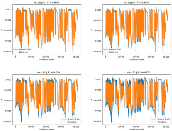
Figure 8. Channel-wise surrogate: u-displacement predictions vs. COMSOL ground truth for strides $h\in \{4,8,16,32\}$.

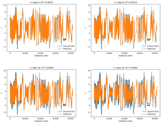
Figure 9. Channel-wise surrogate: v-displacement predictions vs. COMSOL ground truth for strides $h\in \{4,8,16,32\}$.

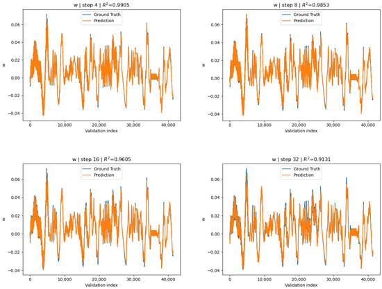
Figure 10. Channel-wise surrogate: w-displacement predictions vs. COMSOL ground truth for strides $h\in \{4,8,16,32\}$.

Table 4. $R^2$ with respect to h for the channel-wise surrogates displacement channels.

h	${\mathit{R}}^2\left(\mathit{u}\right)$	${\mathit{R}}^2\left(\mathit{v}\right)$	${\mathit{R}}^2\left(\mathit{w}\right)$
1	0.9877	0.9863	0.9803
2	0.9918	0.9898	0.9889
4	0.9867	0.9874	0.9906
8	0.9647	0.9716	0.9854
16	0.8601	0.8857	0.9608
32	0.6337	0.6996	0.9132
64	0.4521	0.5626	0.8531
100	0.3128	0.4441	0.7764

Therefore, both surrogates’ v-channel accuracy is within the empirically observed accuracy difference between COMSOL FEA on PZT s-drives and experimental validation (≈ 5%) [12] for $h\le 8$. The key difference between the two is that, while the global-norm variant exhibits marginally higher accuracies on v-channel displacement exclusively, the channel-wise variant is within the accepted accuracy range for all three displacement channels.

3.2. Surrogate Runtime Performance

Apart from accuracy under varying strides, we analyze how end-to-end runtime scales with respect to h on our channel-wise surrogate. We observe that stride selections introduce significant changes in simulation runtime and accuracy (see Figure 8, Figure 9, Figure 10 and Figure 11). We execute our runtime evaluation script using the SLURM workload manager with 32 cores from two AMD EPYC 7F72 24-Core Processors @3.2 GHz, an NVIDIA Tesla A40 with 48 GB of VRAM, and 124 GB of memory, on the full validation set for fixed strides $h\in \Omega$.

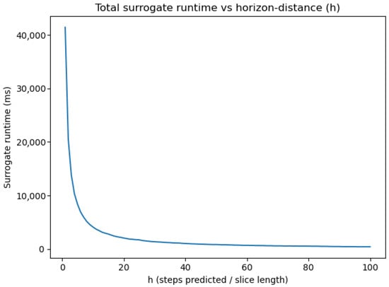
Figure 11. Surrogate-evaluation runtime (ms) vs. horizon length.

We found that the low fidelity run: $h=100$ took $0.4$ s to finish, while the high fidelity run: $h=1$ took a total of $40.8$ s. From our results, we observe a monotonically decreasing curve with a steep initial drop for small horizon distances in Figure 11, showing the strong anti-correlation between runtime and stride-length.

3.3. Multi-Surrogate Runtime Performance

Instantiating our model into a multi-surrogate setup, we push a single surrogate into two NVIDIA H100’s with 80 GB of VRAM each, 128 GB of 4800 MT/s memory, and 64 cores from $2\times 56$-core Intel Xeon Platinums @$2.0$ Ghz. Concretely, we replicate the trained sequence-to-sequence forecaster once per GPU and execute inference using BF16 autocast on CUDA with TF32-enabled matrix multiplies. Each replica processes a batched set of actuator states in parallel, while a CPU dispatcher assigns shards to devices so that both GPUs remain fully saturated throughout the rollouts. Our end-to-end evaluation script reports (i) total wall-clock time for a full validation set rollout and (ii) effective throughput (samples/second), where a sample denotes one surrogate state advanced by one rollout window.

3.3.1. Tolerance-Driven Stride Selection

To reduce redundant evaluations on horizon rollouts, we reuse the model’s multi-step forecast in chunks. Concretely, given a window prediction for sample i, we compute a per-step RMSE

$$e_{i,t}=\sqrt{{\displaystyle \frac{1}{3}}\sum _{c\in \{u,v,w\}}{\left({\hat{y}}_{i,t,c}-y_{i,t,c}\right)}^2},$$

(25)

and then define the per-sample stride

$$k_i=\left\{\begin{array}{cc}\max \{t:e_{i,t}\le ϵ\}+1,\hfill & \mathrm{if} \mathrm{any} \mathrm{step} \mathrm{under} \mathrm{tolerance},\hfill \\ 1,\hfill & \mathrm{otherwise},\hfill \end{array}\right.$$

(26)

where $ϵ$ is the specified tolerance. We then advance the rolling input buffer by inserting the next k normalized predicted displacement steps and shifting the history window forward. For a rollout of length N, the number of required windows is $\lceil N/k\rceil$; therefore, a smaller k increases the number of required windows and runtime.

Purpose of Tolerance Driven Stride

Note that our tolerance-based stride selection is an oracle benchmarking mechanism because it uses the held-out FEA displacement to choose $k_i$. In deployment, stride selection must be estimated without access to ground truth (either through a learned mechanism or set constant). Our instantiation of a variadic stride system simply serves as an example of how the autoregressive nature of our surrogate can be exploited after training.

3.3.2. Scaling Behavior: Throughput and Simulation Runtime

To characterize scaling, we sweep the batch size over powers of two:

$$\mathrm{batch\_size}\in \{2^1,2^2,\dots ,2^{25}\},$$

(27)

with an $ϵ=0.02$ as a throughput-heavy, accuracy-weak demonstration. Figure 12 and Figure 13 summarize the results. Sequence throughput rapidly increases with batch size as kernel launch overhead decreases and GPU utilization improves: from ≈$2.85\times {10}^2$ samples/s at batch size 2 to ≈$1\times {10}^5$ samples/s by batch size 2048, and reaching ≈$4.17\times {10}^5$ samples/s by batch size $2^{14}$ (16384), a net speedup of ∼$1.46\times {10}^3$. Beyond $2^{14}$, performance plateaus in the range ≈ $4.17\times {10}^5$ samples/s, with only marginal gains from further increases in batch size. Practically, this indicates that once both H100s are saturated, additional batching primarily increases memory costs without meaningful improvement of throughput. Interestingly, we observe a decrease in sample throughput and an increase in runtime around $2^{13}$ followed by a plateau. While the Compute Unified Device Architecture (CUDA) API that allows GPU training is abstracted by many computational layers, we can guess that this decrease is likely caused by a transition in how memory, parallelism, and kernel execution are utilized on the GPU as the problem size crosses key architectural thresholds.

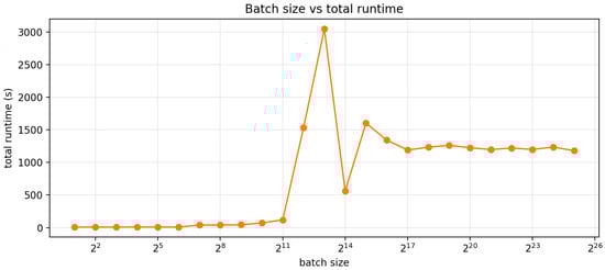
Figure 12. Batch size vs. simulation runtime on 49,988 validation samples.

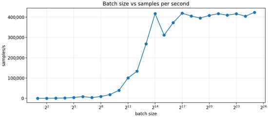
Figure 13. Batch size vs. sample throughput on 49,988 validation samples.

The batch-size sweep exhibits a bi-modal runtime profile because our benchmark couples workload size and rollout length to the dynamically chosen stride length. In each run, the total number of simulated surrogates scales as $S=\min \{N_{val},2·\mathrm{batch\_size}\}$, while the rollout advances in chunks of length k selected by the tolerance mechanism. Because the end-to-end runtime is easily approximated by $T\propto S·\lceil N_{val}/k\rceil$, the runtime becomes piecewise and can change abruptly even when the median stride differs by only a few points. For example, once S saturates at the full validation set, a stride of $k=5$, requires $\lceil \left|N_{val}\right|/5\rceil$ windows, whereas a modest reduction to $k=2$ increases this to $\lceil \left|N_{val}\right|/2\rceil$ windows, and the degenerate case $k=1$ forces $|N_{val}|$ windows, producing a sharp wall-clock spike despite similar per-window GPU throughput. Conversely, where the tolerance mechanism permits larger strides, e.g., $k=32$, the same rollout only requires $\lceil \left|N_{val}\right|/32\rceil$ windows, yielding an order-of-magnitude reduction in total runtime, albeit with significant error. Despite this great variance, there is still a strong correlation between batch size and runtime. Importantly, there is no “one size fits all” stride selection method. On the surface, this seems like a limitation; however, this framework can be tailored both for extremely large-scale, high-throughput simulations involving millions of actuators and for small-scale analyses that closely reproduce transient finite element responses under tighter stride or tolerance settings.

For completeness, we also show the mean stride length for 128 values of $ϵ$ spanning $[{10}^{-4},1]$ in Figure 14. The curve begins with a sharp increase in mean stride and then approaches a horizontal asymptote as $ϵ$ approaches 1.

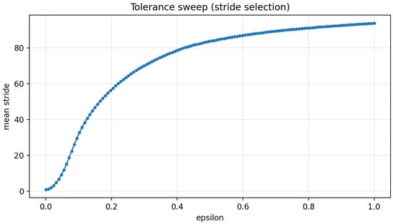
Figure 14. Mean tolerance driven stride for 128 values of $ϵ$ spanning $[{10}^{-4},1]$.

4. Discussion

The following discussion interprets the results in terms of fidelity to transient finite element simulations, the computational tradeoffs enabled by data-driven surrogate modeling, possible future applications, and works.

Using GPU hardware, we can now predict the dynamic response of over 67 million independent actuators in minutes, whereas traditional PDE solvers like COMSOL are simply unable to solve or even construct such systems. Despite this, FEA tools like COMSOL and ANSYS remain invaluable due to their ease-of-use, non-intrusiveness, and grounding in constitutive equations. In summary, by trading off marginal accuracy with respect to numerical methods, we have shown substantial gains in computational throughput and minimizing FEA’s curse of dimensionality through reduced order modeling.

Mechanical Coupling

Importantly, we do not introduce built-in mechanical coupling; each sample in the batch instantiates a single “black box” that predicts actuator displacement. Often, different mechanical coupling mechanisms are ill-suited for different problems, making the universality of the surrogate valuable. During FEA, we pass external traction loads to the actuator, giving it the ability to be mechanically coupled with further augmentation. The following, in principle, can be used in tandem with our surrogate to massively accelerate large-scale assembly simulation:

• Lumped mass-spring-damper networks: By treating each actuator’s free shuttle as a node with 3 DOFs or just the v displacement channel, connect neighboring nodes with springs/dampers representing the compliant material between actuators. This network, in principle, could model the mechanical coupling between actuator-surrogate assemblies. Furthermore, it would scale linearly with the number of actuators and would exploit massive GPU parallelization.
• Skin/Plate Model: As seen in Figure 15 and Figure 16, the axial-configuration of the s-drive requires several actuators per layer. We can exploit this by treating each slice as a continuous layer where actuators apply point/patch loads and plate deformation gives back reaction forces on each actuator’s location.
  

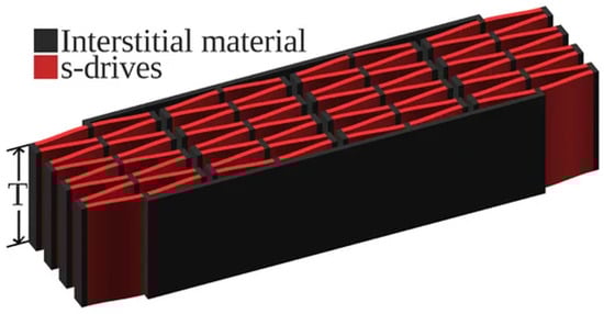  Figure 15. S-drive-based muscle design [5].
  

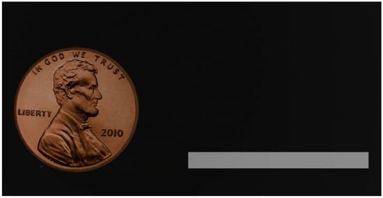  Figure 16. Visualization of an actuator array ($6\times 1042\times 24$) alongside a U.S. penny for scale. Full video available at https://youtu.be/eyIukrxz_YM?si=1i4F-cFcoKplFSmO (accessed on 31 July 2025).
• Coarse Global FEM + Localized Surrogates: Using a reduced-order structural mechanics model, for the whole array, each actuator represents an “active element” where the input-output laws are supplied by the surrogate, and the global solver enforces equilibrium. This surrogate-FEM middle-ground allows for iterative design through intuitive and user-friendly UI, superior scaling than that of full-FEA, and is massively accelerated by GPUs.

Our surrogate unlocks a range of tasks that were previously infeasible with direct finite element analysis. Among them are the following:

• Model-Based Reinforcement Learning (MBRL) Direct policy optimization on finite-element models is computationally prohibitive: single transient FEA simulations can take minutes, hours, or even days depending on model size and parameters, making the millions of interactions required by reinforcement learning infeasible. Despite the poor runtime with these models, they are greatly limited by how many degrees of freedom they need to solve, limiting them to smaller-scale assemblies. In contrast, our surrogate can serve as a component-wise dynamics model in an MBRL loop, making predictions in milliseconds, reducing runtimes significantly, and allowing for large-scale assemblies. This dramatic speedup, combined with a highly portable neural network, makes policy optimization practical for piezoelectric microactuator-based systems.
• Architecture Search Parker et al. demonstrated the feasibility of architecture search in piezoelectric microactuator design, performing systematic sweeps of electrode width, passive-region width, and layer thickness via finite-element analysis to identify geometries that maximize in-plane deflection [45]. Their study highlights the viability and importance of autonomous exploration of geometry search spaces on piezoelectric microactuator-based systems. While focusing on single s-drive optimization, a full-actuator surrogate could be used to accelerate optimization on actuator assemblies.
  Cheney et al. demonstrated that compositional-pattern-producing networks (CPPNs) combined with a library of various materials allow for the evolution of optimized morphologies for trivial tasks such as locomotion [46]. In theory, a similar approach could be applied by leveraging this surrogate framework, creating optimal geometries of microactuator-based robots for specific tasks.

Due to the difficulty in manufacturing high-fidelity s-drive microactuators, the surrogate is trained and evaluated exclusively on finite element data; its fidelity reflects consistency with the underlying numerical model and does not capture experimental uncertainties or fabrication-induced variability.

5. Conclusions

We have presented a data-driven surrogate modeling framework for replacing transient finite element simulations with a surrogate that leverages stacked gated recurrent units to predict boundary displacements of piezoelectric microactuators with millisecond-scale latency. By generating a two-stage waveform library and simulating each sequence with high-fidelity COMSOL FEA on a PZT-5H actuator, we compiled a diverse dataset of half a million time steps covering the device’s dynamic envelope. Our GRU models, trained on 32-step sliding windows of normalized displacements and interpolated load values, achieve millisecond-scale inference per rollout window when reproducing transient finite element responses and are easily parallelizable on GPU hardware.

Future work will focus on mechanical coupling, fabrication methods, empirical validation, and realizing intelligent s-drive-based actuator systems. Through reinforcement learning and genetic search, we aim to create intelligent microrobots, blurring the lines between artificial and biological systems. Before this, much work needs to be conducted on streamlining the fabrication process of these microstructures and designing surrogate frameworks that perform as closely as possible to their real-world counterparts.

References

- Rugar, D.; Hansma, P. Atomic Force Microscopy. Phys. Today 1990, 43, 23–30. [Google Scholar] [CrossRef]
- Bußmann, A.B.; Durasiewicz, C.P.; Kibler, S.H.A.; Wald, C.K. Piezoelectric titanium based microfluidic pump and valves for implantable medical applications. Sens. Actuators A Phys. 2021, 323, 112649. [Google Scholar] [CrossRef]
- Mangi, M.A.; Elahi, H.; Ali, A.; Jabbar, H.; Aqeel, A.B.; Farrukh, A.; Bibi, S.; Altabey, W.A.; Kouritem, S.A.; Noori, M. Applications of piezoelectric-based sensors, actuators, and energy harvesters. Sens. Actuators Rep. 2025, 9, 100302. [Google Scholar] [CrossRef]
- Chigullapalli, A.; Clark, J.V. Extremely Large Deflection Actuators for Translation or Rotation. In Volume 9: Micro- and Nano-Systems Engineering and Packaging, Parts A and B; ASME International Mechanical Engineering Congress and Exposition; ASME: New York, NY, USA, 2012. [Google Scholar] [CrossRef]
- Jones, N.A.; Clark, J. Analytical Modeling and Simulation of S-Drive Piezoelectric Actuators. Actuators 2021, 10, 87. [Google Scholar] [CrossRef]
- Nikolopoulos, S.; Kalogeris, I.; Papadopoulos, V. Non-intrusive Surrogate Modeling for Parametrized Time-dependent PDEs using Convolutional Autoencoders. arXiv 2021, arXiv:2101.05555. [Google Scholar] [CrossRef]
- Kohar, C.P.; Greve, L.; Eller, T.K.; Connolly, D.S.; Inal, K. A machine learning framework for accelerating the design process using CAE simulations: An application to finite element analysis in structural crashworthiness. Comput. Methods Appl. Mech. Eng. 2021, 385, 114008. [Google Scholar] [CrossRef]
- Su, G.; Peng, L.; Hu, L. A Gaussian process-based dynamic surrogate model for complex engineering structural reliability analysis. Struct. Saf. 2017, 68, 97–109. [Google Scholar] [CrossRef]
- Meethal, R.E.; Obst, B.; Khalil, M.; Ghantasala, A.; Kodakkal, A.; Bletzinger, K.U.; Wüchner, R. Finite Element Method-enhanced Neural Network for Forward and Inverse Problems. Adv. Model. Simul. Eng. Sci. 2023, 10, 6. [Google Scholar] [CrossRef]
- Wang, Y.; Zhou, M.; Hou, D.; Cao, W.; Huang, X. Composite Data Driven-Based Adaptive Control for a Piezoelectric Linear Motor. IEEE Trans. Instrum. Meas. 2022, 71, 3527912. [Google Scholar] [CrossRef]
- Makarem, S.; Delibas, B.; Koc, B. Data-Driven Tuning of PID Controlled Piezoelectric Ultrasonic Motor. Actuators 2021, 10, 148. [Google Scholar] [CrossRef]
- Chigullapalli, A. Modeling and Validation of S-Drive: A Nestable Piezoelectric Actuator. Ph.D. Thesis, Purdue University, West Lafayette, IN, USA, 2014. [Google Scholar]
- PolyK Technologies. 8 µm Thick Piezo PVDF Film with 30 nm Thick Aluminum Electrode. 2026. Available online: https://piezopvdf.com/8-um-pvdf-film-aluminum-electrode/ (accessed on 15 January 2026).
- PolyK Technologies. PVDF Poled Piezoelectric Film, 120 mm × 120 mm, Platinum Electrode Both Surfaces, Uniaxially Oriented with High d31. 2026. Available online: https://piezopvdf.com/pvdf-piezo-Pt/ (accessed on 15 January 2026).
- Hake, A.E.; Zhao, C.; Sung, W.K.; Grosh, K. Design and Experimental Assessment of Low-Noise Piezoelectric Microelectromechanical Systems Vibration Sensors. IEEE Sens. J. 2021, 21, 17703–17711. [Google Scholar] [CrossRef]
- Hooker, M.W. Properties of PZT-Based Piezoelectric Ceramics Between − 150 and 250 C. 1998. Available online: https://ntrs.nasa.gov/citations/19980236888 (accessed on 15 January 2026).
- PIEZO.COM. PZT5A & 5H Materials Technical Data (Typical Values). Available online: https://info.piezo.com/hubfs/Data-Sheets/piezo-PZT-5A_PZT-5H-material-properties.pdf (accessed on 15 January 2026).
- Zhou, C.; Zhang, J.; Yao, W.; Liu, D.; He, G. Remarkably strong piezoelectricity, rhombohedral-orthorhombic-tetragonal phase coexistence and domain structure of (K,Na)(Nb,Sb)O3–(Bi,Na)ZrO3–BaZrO3 ceramics. J. Alloys Compd. 2020, 820, 153411. [Google Scholar] [CrossRef]
- Raul Alin, B.; Badea, I.; Bucur, A.I.; Novaconi, S. Good Quality Factor in GdMnO3-Doped (K0.5Na0.5)NbO3 Piezoelectric Ceramics. J. Electron. Mater. 2016, 45, 3046–3052. [Google Scholar] [CrossRef]
- Zheng, M.; Hou, Y.; Chao, L.; Zhu, M. Piezoelectric KNN ceramic for energy harvesting from mechanochemically activated precursors. J. Mater. Sci. Mater. Electron. 2018, 29, 9582–9587. [Google Scholar] [CrossRef]
- Bhadwal, N.; Ben Mrad, R.; Behdinan, K. Review of Piezoelectric Properties and Power Output of PVDF and Copolymer-Based Piezoelectric Nanogenerators. Nanomaterials 2023, 13, 3170. [Google Scholar] [CrossRef]
- Xia, W.; Zhang, Z. PVDF-based dielectric polymers and their applications in electronic materials. IET Nanodielectr. 2018, 1, 17–31. [Google Scholar] [CrossRef]
- Taleb, S.; Badillo-Ávila, M.A.; Acuautla, M. Fabrication of poly (vinylidene fluoride) films by ultrasonic spray coating; uniformity and piezoelectric properties. Mater. Des. 2021, 212, 110273. [Google Scholar] [CrossRef]
- Li, J.F. Lead-Free Piezoelectric Materials; Wiley-VCH: Weinheim, Germany, 2021. [Google Scholar]
- Wang, R.; Tang, E.; Yang, G.; Han, Y.; Chen, C. Discharge characteristics of fractured soft piezoelectric ceramics under repeated impact. Ceram. Int. 2020, 46, 23499–23504. [Google Scholar] [CrossRef]
- Wang, R.; Tang, E.; Yang, G.; Han, Y. Experimental research on dynamic response of PZT-5H under impact load. Ceram. Int. 2020, 46, 2868–2876. [Google Scholar] [CrossRef]
- Chung, J.; Gülçehre, Ç.; Cho, K.; Bengio, Y. Empirical Evaluation of Gated Recurrent Neural Networks on Sequence Modeling. arXiv 2014, arXiv:1412.3555. [Google Scholar] [CrossRef]
- Hochreiter, S.; Schmidhuber, J. Long Short-Term Memory. Neural Comput. 1997, 9, 1735–1780. [Google Scholar] [CrossRef] [PubMed]
- Vaswani, A.; Shazeer, N.; Parmar, N.; Uszkoreit, J.; Jones, L.; Gomez, A.N.; Kaiser, L.; Polosukhin, I. Attention Is All You Need. arXiv 2017, arXiv:1706.0376. [Google Scholar] [CrossRef]
- Jumper, J.; Evans, R.; Pritzel, A.; Green, T.; Figurnov, M.; Ronneberger, O.; Tunyasuvunakool, K.; Bates, R.; Žídek, A.; Potapenko, A.; et al. Highly accurate protein structure prediction with AlphaFold. Nature 2021, 596, 583–589. [Google Scholar] [CrossRef] [PubMed]
- Brohan, A.; Brown, N.; Carbajal, J.; Chebotar, Y.; Chen, X.; Choromanski, K.; Ding, T.; Driess, D.; Dubey, A.; Finn, C.; et al. RT-2: Vision-Language-Action Models Transfer Web Knowledge to Robotic Control. arXiv 2023, arXiv:2307.15818. [Google Scholar] [CrossRef]
- Mohan, A.T.; Gaitonde, D.V. A Deep Learning based Approach to Reduced Order Modeling for Turbulent Flow Control using LSTM Neural Networks. arXiv 2018, arXiv:1804.09269. [Google Scholar] [CrossRef]
- Halder, R.; Damodaran, M.; Cheong, K.B. Deep Learning-Driven Nonlinear Reduced-Order Models for Predicting Wave-Structure Interaction. arXiv 2023, arXiv:2301.11835. [Google Scholar] [CrossRef]
- Ahmed, S.E.; San, O.; Rasheed, A.; Iliescu, T. A long short-term memory embedding for hybrid uplifted reduced order models. Phys. D Nonlinear Phenom. 2020, 409, 132471. [Google Scholar] [CrossRef]
- Lazzara, M.; Chevalier, M.; Colombo, M.; Garay Garcia, J.; Lapeyre, C.; Teste, O. Surrogate modelling for an aircraft dynamic landing loads simulation using an LSTM AutoEncoder-based dimensionality reduction approach. Aerosp. Sci. Technol. 2022, 126, 107629. [Google Scholar] [CrossRef]
- Dave, H.; Cotteleer, L.; Parente, A. Physics-informed non-intrusive reduced-order modeling of parameterized dynamical systems. Comput. Methods Appl. Mech. Eng. 2025, 443, 118045. [Google Scholar] [CrossRef]
- Yang, J.; Faverjon, B.; Peters, H.; Kessissoglou, N. Application of Polynomial Chaos Expansion and Model Order Reduction for Dynamic Analysis of Structures with Uncertainties. Procedia IUTAM 2015, 13, 63–70. [Google Scholar] [CrossRef]
- Hensman, J.; Fusi, N.; Lawrence, N.D. Gaussian Processes for Big Data. arXiv 2013, arXiv:1309.6835. [Google Scholar] [CrossRef]
- Park, K.; Allen, M.S. A Gaussian process regression reduced order model for geometrically nonlinear structures. Mech. Syst. Signal Process. 2023, 184, 109720. [Google Scholar] [CrossRef]
- Gobat, G.; Opreni, A.; Fresca, S.; Manzoni, A.; Frangi, A. Reduced order modeling of nonlinear microstructures through Proper Orthogonal Decomposition. Mech. Syst. Signal Process. 2022, 171, 108864. [Google Scholar] [CrossRef]
- Chatpattanasiri, C.; Franzetti, G.; Bonfanti, M.; Diaz-Zuccarini, V.; Balabani, S. Towards Reduced Order Models via Robust Proper Orthogonal Decomposition to capture personalised aortic haemodynamics. J. Biomech. 2023, 158, 111759. [Google Scholar] [CrossRef]
- Bai, Z.; Bindel, D.; Clark, J.; Demmel, J.; Pister, K.; Zhou, N. New numerical techniques and tools in SUGAR for 3D MEMS simulation. In Proceedings of the Fourth Technical International Conference on Modeling and Simulation of Microsystems, Hilton Head Island, SC, USA, 19–21 March 2001. [Google Scholar]
- Padoan, A.; Forni, F.; Sepulchre, R. Balanced truncation for model reduction of biological oscillators. Biol. Cybern. 2021, 115, 383–395. [Google Scholar] [CrossRef]
- Kingma, D.P.; Ba, J. Adam: A Method for Stochastic Optimization. arXiv 2017, arXiv:1412.6980. [Google Scholar] [CrossRef]
- Megginson, P.; Clark, J.; Clarson, R. Optimizing the Electrode Geometry of an In-Plane Unimorph Piezoelectric Microactuator for Maximum Deflection. Modelling 2024, 5, 1084–1100. [Google Scholar] [CrossRef]
- Cheney, N.; MacCurdy, R.; Clune, J.; Lipson, H. Unshackling Evolution: Evolving Soft Robots with Multiple Materials and a Powerful Generative Encoding. In Proceedings of the 15th Annual Conference on Genetic and Evolutionary Computation, Amsterdam, The Netherlands, 6–10 July 2013. [Google Scholar] [CrossRef]
Disclaimer/Publisher’s Note: The statements, opinions and data contained in all publications are solely those of the individual author(s) and contributor(s) and not of MDPI and/or the editor(s). MDPI and/or the editor(s) disclaim responsibility for any injury to people or property resulting from any ideas, methods, instructions or products referred to in the content. |
© 2026 by the authors. Licensee MDPI, Basel, Switzerland. This article is an open access article distributed under the terms and conditions of the Creative Commons Attribution (CC BY) license.