Predefined-Time Tracking Control of Servo Hydraulic Cylinder Based on Reinforcement Learning

Abstract

Electro-hydraulic servo systems are characterized by significant nonlinearities. Reinforcement learning (RL), known for its model-free nature and adaptive learning capabilities, presents a promising approach for handling uncertainties inherent in such systems. This paper proposes a predefined-time tracking control scheme based on RL, which achieves fast and accurate tracking performance. The proposed design employs an actor–critic neural network strategy to actively compensate for system uncertainties. Within a conventional backstepping framework, a command-filtering technique is integrated to construct a predefined-time control structure. This not only circumvents the issue of differential explosion but also guarantees system convergence within a predefined time, which can be specified independently by the designer. Simulation results and comparisons validate the enhanced control performance of the proposed controller.

1. Introduction

Electro-hydraulic servo systems are extensively utilized in defense and various critical industrial sectors owing to their prominent advantages, including high power density, strong load stiffness, and large output force/torque. These systems play a pivotal role in control and power transmission applications [1,2,3,4]. However, their complex dynamics and inherent uncertainties pose significant challenges to further enhancing controller performance. A well-established and powerful paradigm for handling such uncertainties is linear robust control. This approach typically seeks to derive a linear model representation of the system—either through physical model linearization or data-driven identification—and explicitly quantifies the discrepancies between this nominal model and the true nonlinear plant as bounded uncertainties. These uncertainties can be structured or unstructured and frequency-dependent, encompassing unmodeled dynamics, disturbances, and noise. Robust control theories, such as H∞ synthesis, are then employed to design controllers that guarantee stability and performance for all plants within the defined uncertainty set, yielding quantifiable robustness margins [5,6]. For instance, Fallahi et al. [5] modeled linearization errors in an electro-hydraulic servo system as a polytopic uncertainty and designed an H∞ controller via Linear Matrix Inequalities, achieving robust position control. Similarly, Lu et al. [6] addressed parameter uncertainties and load disturbances in a valve-controlled hydraulic motor by formulating them as structured norm-bounded uncertainties and developing a robust H∞ tracking controller. A key practical advantage of this paradigm is the direct synthesis of controllers amenable to stable digital implementation, often with favorable numerical properties. Nonetheless, the effectiveness of these linear robust methods can be constrained when applied to highly nonlinear systems. The conservatism introduced by covering all nonlinear behaviors with a linear uncertainty set may limit achievable performance, especially when strict transient performance is required.

To move beyond these limitations and more directly address or compensate for the system’s inherent nonlinearities, the field of advanced control has evolved toward a variety of nonlinear control strategies developed in recent decades, such as sliding mode control [7] and nonlinear robust control [8,9]. Despite their potential, sliding mode control employs high-gain switching feedback to achieve robustness, which introduces high-frequency chattering caused by discontinuous control signals. Similarly, robust control tends to rely on increased feedback gains to suppress disturbances, which may excite unmodeled high-frequency dynamics. Due to insufficient handling of uncertainties, these methods can result in deviations from the desired trajectory, system instability, and even compromised operational safety.

To overcome the limitations induced by high-gain strategies, it is essential to develop high-performance controllers capable of effectively suppressing or actively compensating for the influence of uncertainties on system performance. The robust integral of the sign of the error (RISE) controller [10,11] guarantees asymptotic tracking performance owing to the strong robustness of its integral robust control law against smooth time-varying disturbances. Nevertheless, the nonlinear robust gain in this controller depends critically on the upper bounds of the first and second time derivatives of the system uncertainties. Observer-based control methods, such as the Extended State Observer (ESO) [12,13] and the Disturbance Observer [14,15], circumvent high-gain feedback by estimating and proactively compensating for uncertainties. Additionally, leveraging the universal function approximation property of neural networks, researchers have successfully addressed a wide range of control problems involving unknown system dynamics [16,17]. It should be noted, however, that although these controllers demonstrate effective uncertainty handling, their performance remains inherently constrained by the accuracy of the system model due to their reliance on prior model knowledge.

Overcoming the limitations of traditional nonlinear control’s reliance on dynamic models, learning-based control strategies have emerged as viable alternatives, generating substantial interest in the research community. As a representative methodology, reinforcement learning (RL) eliminates the need for explicit mathematical models by autonomously learning optimal control policies through environmental interaction [18,19]. A prominent implementation of this approach is the actor–critic RL framework, where the actor network generates control decisions through environmental interaction, while the critic network evaluates these decisions and guides the actor’s updates via policy gradient feedback to enhance overall system performance. Nevertheless, it should be acknowledged that completely abandoning model-based structures presents significant challenges for controller adaptation in complex operational scenarios. In [20], an actor–critic RL-based optimal control scheme was developed to enhance tracking performance for unmanned surface vehicles exhibiting complex unknown nonlinearities. Another study [21] integrated reinforcement learning with a sliding mode observer design, achieving spacecraft attitude stabilization control within a conventional backstepping framework. Notably, these approaches effectively leverage nonlinear control theory to establish crucial guarantees for stability, safety, and convergence during the RL process. Similar integrations of intelligent decision-making with system dynamic stability have been successfully demonstrated in studies [22,23].

Another core challenge in electro-hydraulic servo systems involves achieving sufficiently fast response times. To address transient performance requirements, finite-time control methodologies have been developed to ensure system state stabilization within an estimable time frame. The authors of [24] developed an observer-based finite-time controller for hydraulic actuators with complex unknown dynamics, while [25] incorporated dynamic surface control to achieve high-precision finite-time control of hydraulic manipulators without complexity explosion. A notable limitation of these approaches, however, is their convergence time dependence on initial system conditions. To overcome this, ref. [26] proposed a fixed-time disturbance observer-based controller for electro-hydraulic systems under input saturation constraints. In an innovative extension, ref. [27] combined fixed-time control with reinforcement learning for spacecraft attitude consensus control, with a similar hybrid approach applied to manipulator control in [28]. Despite these advances, the convergence time upper bounds in such methods remain conservatively tuned through design parameters. To tackle these challenges, the predefined-time control concept introduced in [29] becomes the focus of this paper, as it allows arbitrary pre-specification of the system convergence time, independent of initial states or design parameters. Furthermore, the motivation of this work stems from effectively integrating the data-driven optimization capabilities of reinforcement learning with predefined-time control, thereby compensating for the limitations of predefined-time methods in handling complex uncertainties in electro-hydraulic servo systems.

Building upon the insights from the preceding discussion, this paper investigates the integration of reinforcement learning with predefined-time control to address trajectory tracking challenges in electro-hydraulic servo systems with complex nonlinearities. The proposed methodology employs an actor–critic neural network-based reinforcement learning strategy to actively identify and compensate for system uncertainties within the control design. Developed upon a command-filtered backstepping structure, the resulting predefined-time control framework ensures system convergence within a user-specified time. The main contributions of this work are summarized as follows:

• A predefined-time control framework is established for electro-hydraulic servo systems, guaranteeing predefined-time convergence of position tracking errors. The system convergence time is independent of initial states and requires no complex parameter computation.
• An intelligent integration of the actor–critic reinforcement learning framework effectively handles system uncertainties, thereby relaxing conventional assumptions regarding known uncertainty bounds or bounded derivatives.
• A novel nonsingular predefined-time command filter is utilized, which not only circumvents complexity explosion issues arising from repeated differentiation in backstepping design but also maintains continuity and non-singularity throughout the subsequent controller development.

The remainder of this paper is structured as follows. Section 2 presents the problem formulation and necessary preliminaries. The design of the RL-based predefined-time controller and its corresponding stability analysis are detailed in Section 3. Section 4 provides comprehensive simulation results and discussions. Finally, Section 5 concludes the paper with a summary of the main findings and contributions.

2. Problem Statement and Preliminaries

The configuration of the electro-hydraulic servo system considered in this study is shown in Figure 1, where a valve-controlled double-rod hydraulic cylinder directly drives an inertial load.

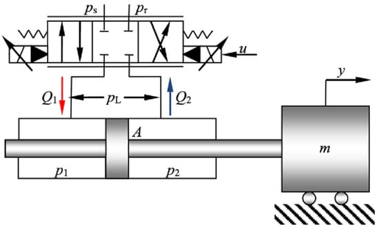
Figure 1. Schematic diagram of the electro-hydraulic servomechanism.

The dynamic equation governing the inertial load is expressed as:

$$m\ddot{y}=P_{L}A-F_f(y,\dot{y},\ddot{y},t)$$

(1)

where $m$ is the mass of the inertial load, $y$ denotes the displacement of the inertial load, $P_L$ represents the pressure difference across the hydraulic cylinder, $A$ is the effective piston area, and $F_f(y,\dot{y},\ddot{y},t)$ signifies the unknown mechanical dynamics of the system.

The pressure dynamics of the hydraulic actuator are governed by the following equation:

$$\frac{V_t}{4{\beta }_e}{\dot{P}}_L=-A\dot{y}-C_t{P}_L+Q_L+q(t)$$

(2)

where $V_t$ is the total control chamber volume, ${\beta }_e$ represents the effective bulk modulus of the hydraulic system, describing the combined deformability of the hydraulic oil and the hydraulic lines, $C_t$ represents the total leakage coefficient, $Q_L$ is the load flow, and $q(t)$ signifies the model uncertainties arising from complex internal leakage, parameter uncertainties, and unmodeled dynamic effects.

Remark 1.

In hydraulic systems, the compressibility of the fluid affects the system’s response speed, stiffness, and control accuracy. For high-dynamic-response systems, compressibility must be strictly controlled, making both pipeline rigidity and the bulk modulus of the hydraulic oil critically important. Here, we define the effective bulk modulus, ${\beta }_e$, which describes the combined deformability of the hydraulic oil and the hydraulic lines. When the hydraulic lines are rigid, the deformation of the pipeline is negligible compared to that of the hydraulic oil itself. In such cases, it can be assumed that the bulk modulus describes only the susceptibility to deformation of the hydraulic oil. This simplification is a common assumption in engineering practice.

Neglecting spool dynamics, the load flow equation of the servo valve is given by:

$$Q_L=k_{q}u\sqrt{P_s-sign(u)P_L}$$

(3)

where $P_s$ is the constant supply pressure, $u$ denotes the system control input, the flow gain is defined as $k_q=C_{d}w\sqrt{1/\rho }$, $C_d$ is the discharge coefficient, $w$ represents the spool valve area gradient, $\rho$ is the fluid density, and the sign function $sign(u)$ is given by:

$$sign(u)=\left\{\begin{array}{cc}1,& u\ge 0\\ -1,& u<0\end{array}\right.$$

(4)

For the controller design objective, the mathematical model of the electro-hydraulic system is expressed in state-space form. The state vector is defined as x = [x₁, x₂, x₃]^T = [$y$, $\dot{y}$, $A{P}_L$/m]^T. This formulation yields:

$$\left\{\begin{array}{l}{\dot{x}}_1=x_2\\ {\dot{x}}_2=x_3-F\\ {\dot{x}}_3=gu-{\phi }_1{x}_2-{\phi }_2{x}_3+d\end{array}\right.$$

(5)

where $g=4{\beta }_{e}A{k}_u\sqrt{P_s-sign(u)m{x}_3/A}/m/V_t$, $F=F_f(y,\dot{y},\ddot{y},t)/m$, ${\phi }_1=4{\beta }_{e}A/m/V_t$, ${\phi }_2= 4{\beta }_e{C}_t/V_t$, and $d= 4{\beta }_{e}Aq\left(t\right)/\left(m{V}_t\right)$.

The control objective is to design a continuous control input that ensures accurate tracking of a prescribed smooth trajectory by the load position under the following assumptions, while guaranteeing predefined-time convergence performance for the hydraulic system subject to unknown dynamics and disturbances:

Assumption 1.

The desired motion trajectory for the system is twice continuously differentiable and bounded.

Assumption 2.

The system uncertainty is bounded, satisfying $|d|\le \delta$, where $\delta$ is an unknown positive constant.

3. Reinforcement Learning-Based Predefined-Time Controller Design

3.1. Preliminaries

The following preliminaries must be established prior to the controller design:

Lemma 1

([30]). Consider a continuously differentiable Lyapunov function candidate $V_x$ satisfying

$$V_x\ge 0 \mathrm{and} {\dot{V}}_x\le -\frac{2}{\rho T_c{\mathcal{l}}^{\prime }}(2{\mathcal{l}}^{\prime }{V}_x+{\mathcal{l}}_1{V_x}^{1-\frac{\rho }{2}}+{\mathcal{l}}_2{V_x}^{1+\frac{\rho }{2}})+S$$

(6)

where $S$, $\rho$, ${\mathcal{l}}_1$, ${\mathcal{l}}_2$ and  ${\mathcal{l}}^{\prime }$ are constants such that $0<S<\infty$, $0<\rho <1$, ${\mathcal{l}}_1>0$, ${\mathcal{l}}_2>0$ and ${\mathcal{l}}^{\prime }=\sqrt{{\mathcal{l}}_1{\mathcal{l}}_2}>0$. Then, the closed-loop system achieves predefined-time practical stability. Specifically, the control system converges to a bounded region within a predefined time parameter  $T_c$ that can be arbitrarily selected.

Lemma 2

([28]). Based on the universal approximation capability of neural networks, a continuous function $N(X)$ can be represented in the form:

$$N(X)=w^T\varphi (X)+\kappa$$

(7)

where$w ={[w_1, w_2, \dots , w_v]}^T$ represents the ideal weight vector, with  $v>1$ indicating the number of neurons in the hidden layer,  $X={[X_1, X_2, \dots , X_n]}^T\in {ℝ}^n$ denotes the input vector;  $\kappa$ represents the approximation error, and the activation function $\varphi (X)$ employs the Gaussian function as specified in [28].

To mitigate the potential issue of “complexity explosion” in the third-order electro-hydraulic servo system, a nonsingular predefined-time differentiator is incorporated into the subsequent controller synthesis. Its structure is given as follows [31]:

$${\dot{\widehat{\alpha }}}_i=-\frac{\pi }{2^{\frac{\zeta }{2}}\zeta T_c}{({\widehat{\alpha }}_i-{\alpha }_i)}^{1+\zeta }-\frac{\pi }{2^{1-\frac{\zeta }{2}}\zeta T_c}{({\widehat{\alpha }}_i-{\alpha }_i)}^{1-\zeta }\tanh (\frac{{({\widehat{\alpha }}_i-{\alpha }_i)}^{2-\zeta }}{\varsigma }),{\widehat{\alpha }}_i(0)={\alpha }_i(0)$$

(8)

where i = 1, 2; ζ is defined as a positive adjustable constant constrained by 0 < ζ < 1; ${\alpha }_i$ (the virtual control law) acts as the filter input; ${\widehat{\alpha }}_i$ constitutes the filter output; and $T_c$ serves as the adjustable parameter that determines the predefined convergence time.

3.2. Actor–Critic Network Design

This section designs actor–critic networks to cope with unknown nonlinear dynamics in the system. The critic network serves to assess control performance, and the actor network functions to approximate the unknown dynamics.

Critic Network: Through the evaluation of the current control policy’s execution cost, the estimated value is leveraged to provide feedback, thereby directing policy optimization. The long-term cost function is defined as follows:

$$V_c(t)={\int }_t^{\infty }{e}^{-\upsilon (\tau -t)}h(\tau )d\tau$$

(9)

where $\upsilon$ serves as the discount factor to guarantee the boundedness of the cost function, and $h(\tau )$ represents the instantaneous cost function:

$$h(t)={{\xi }_1}^2+{{\alpha }_2}^2$$

(10)

where ${\xi }_1$ denotes the error compensation signal, and ${\alpha }_2$ represents the second-order virtual control signal (see Section 3.3 for detailed definitions).

Based on Equation (9), the Bellman equation is derived as:

$$\upsilon V_c=h(t)+{\dot{V}}_c$$

(11)

Following Lemma 2, a neural network is employed to approximate the cost function, yielding the relations $V_c={w_c}^T{\varphi }_c({\xi }_1)+{\kappa }_c$ and the approximation ${\widehat{V}}_c={{\widehat{w}}_c}^T{\varphi }_c({\xi }_1)$, where ${\widehat{w}}_c$ denote the estimate of $w_c$, obtained by minimizing the following objective function: $E_c=0.5{e_c}^2$, with $e_c=h(t)+{\dot{\widehat{V}}}_c-\upsilon {\widehat{V}}_c$.

The update rule for the critic network is designed in accordance with the gradient descent method:

$${\dot{\widehat{W}}}_c=-{\delta }_c(h(t)+{{\widehat{W}}_c}^T\mathrm{\Lambda })\mathrm{\Lambda }$$

(12)

where ${\delta }_c$ represents the adjustable gain, the intermediate variable $\mathrm{\Lambda }=-\upsilon {\varphi }_c({\xi }_1)+\nabla {\varphi }_c\cdot {\dot{\xi }}_1$, and $\nabla {\varphi }_c$ denotes the gradient of ${\varphi }_c$.

Actor Network: According to Lemma 2, an actor neural network is employed to approximate the unknown dynamics $F={w_a}^T{\varphi }_a(X_a)+{\kappa }_a$, which, can be expressed in the following approximate form:

$$\widehat{F}={{\widehat{w}}_a}^T{\varphi }_a(X_a)$$

(13)

where ${\widehat{w}}_a$ denote the estimate of $w_a$, obtained by minimizing the following objective function: $E_a=0.5{e_a}^2$, with $e_a=K_V{\widehat{V}}_c({\xi }_1)+\tilde{F}$, and $K_V$ represents the adjustable gain, $\tilde{F}=\widehat{F}-F={\tilde{w}}_a{\varphi }_a(X_a)-{\kappa }_a$.

The update rule for the actor network is designed in accordance with the gradient descent method:

$${\dot{\widehat{w}}}_a=-{\delta }_a(K_V{\widehat{V}}_c({\xi }_1)+\tilde{F}){\phi }_a(X_a)$$

(14)

where ${\delta }_a$ represents the adjustable gain.

The parameter projection approach guarantees bounded neural network weights, that is, $||{\widehat{W}}_c||\le {\overline{W}}_c$ and $||{\widehat{W}}_a||\le {\overline{W}}_a$. The update algorithm can be configured as follows:

$$\begin{array}{l}{\dot{\widehat{W}}}_c=\left\{\begin{array}{l}-{\delta }_c(h(t)+{{\widehat{W}}_c}^T\mathrm{\Lambda })\mathrm{\Lambda }, ||{\widehat{W}}_c||<||{\overline{W}}_c||or||{\widehat{W}}_c||=||{\overline{W}}_c||, {{\widehat{W}}_c}^T(h(t)+{{\widehat{W}}_c}^T\mathrm{\Lambda })\mathrm{\Lambda }>0\\ -{\delta }_c(h(t)+{{\widehat{W}}_c}^T\mathrm{\Lambda })\mathrm{\Lambda }+{\delta }_c{\xi }_c, ||{\widehat{W}}_c||=||{\overline{W}}_c||, {{\widehat{W}}_c}^T(h(t)+{{\widehat{W}}_c}^T\mathrm{\Lambda })\mathrm{\Lambda }\le 0\end{array}\right.\\ {\dot{\widehat{W}}}_a=\left\{\begin{array}{l}-{\delta }_a{\rho }_a, ||{\widehat{W}}_a||<||{\overline{W}}_a||or||{\widehat{W}}_a||=||{\overline{W}}_a||, {{\widehat{W}}_a}^T{\rho }_a>0\\ -{\delta }_a{\rho }_a+{\delta }_a{\xi }_a, ||{\widehat{W}}_a||=||{\overline{W}}_a||, {{\widehat{W}}_a}^T{\rho }_a\le 0\end{array}\right.\end{array}$$

(15)

where the intermediate variable ${\rho }_a=(K_V{\widehat{V}}_c({\xi }_1)+\tilde{F}){\phi }_a(X_a)$, ${\xi }_c=(({{\widehat{W}}_c}^T(h(t)+{{\widehat{W}}_c}^T\mathrm{\Lambda })\mathrm{\Lambda })/||{\widehat{W}}_c|{|}^2){\widehat{W}}_c$ and ${\xi }_a=(({{\widehat{W}}_a}^T{\rho }_a)/||{\widehat{W}}_a|{|}^2){\widehat{W}}_a$.

3.3. RL-Based Predefined-Time Controller Design

Based on the established system model, a predefined-time convergent control scheme is developed through a classical backstepping framework integrated with an actor–critic learning network. The design procedure is systematically carried out in the following three steps:

Step 1: Differentiating the error variable $e_1=x_1-x_d$ yields:

$${\dot{e}}_1={\dot{x}}_1-{\dot{x}}_d=x_2-{\dot{x}}_d=e_2+{\widehat{\alpha }}_1-{\dot{x}}_d$$

(16)

With the filtered error ${\widehat{\alpha }}_1-{\alpha }_1$ defined as the input, the filtered error compensator is constructed as follows:

$${\dot{\eta }}_1=({\widehat{\alpha }}_1-{\alpha }_1)+{\eta }_2-{\lambda }_{\eta 11}{\eta }_1-{\lambda }_{\eta 12}{{\eta }_1}^{1+r}$$

(17)

where the filter compensation coefficients are denoted by ${\lambda }_{\eta 11}=\frac{1}{2}\cdot \frac{4}{r{T}_f}+\frac{2-r}{2}{(\frac{1}{2})}^{1-\frac{r}{2}}\cdot \frac{2a_1}{r{T}_f{a}^{\prime }}$, ${\lambda }_{\eta 12}={(\frac{1}{2})}^{1+\frac{r}{2}}\cdot 3^{\frac{r}{2}}\cdot \frac{3a_2}{r{T}_f{a}^{\prime }}$ with parameters $r$, $a_1$ and $a_2$ are constants such that $0<r<1$, $a_1>0$, $a_2>0$ and $a^{\prime }=\sqrt{a_1{a}_2}$ hold. $t_f$ determines the user-specified convergence time.

Differentiating the error compensation signal ${\xi }_1=e_1-{\eta }_1$ on both sides yields:

$${\dot{\xi }}_1={\xi }_2+{\alpha }_1-{\dot{x}}_d+{\lambda }_{\eta 11}{\eta }_1+{\lambda }_{\eta 12}{{\eta }_1}^{1+r}$$

(18)

Accordingly, the virtual control is constructed as follows:

$${\alpha }_1={\dot{x}}_d-\frac{1}{2}{\xi }_1{{\eta }_1}^2-\frac{1}{2}{\xi }_1{{\eta }_1}^{2+2r}-{\lambda }_{e11}{\xi }_1-{\lambda }_{e12}{{\xi }_1}^{1+r}$$

(19)

where the controller coefficients are denoted by ${\lambda }_{e11}=\frac{1}{2}\cdot \frac{4}{r{T}_f}+\frac{2-r}{2}{(\frac{1}{2})}^{1-\frac{r}{2}}\cdot \frac{2a_1}{r{T}_f{a}^{\prime }}$, ${\lambda }_{e12}={(\frac{1}{2})}^{1+\frac{r}{2}}\cdot 5^{\frac{r}{2}}\cdot \frac{2a_2}{r{T}_f{a}^{\prime }}$.

Step 2: Differentiating the error variable $e_2=x_2-{\widehat{\alpha }}_1$ yields:

$${\dot{e}}_2={\dot{x}}_2-{\dot{\widehat{\alpha }}}_1=x_3+F-{\dot{\widehat{\alpha }}}_1=e_3+{\widehat{\alpha }}_2+F-{\dot{\widehat{\alpha }}}_1$$

(20)

With the filtered error ${\widehat{\alpha }}_2-{\alpha }_2$ defined as the input, the filtered error compensator is constructed as follows:

$${\dot{\eta }}_2=({\widehat{\alpha }}_2-{\alpha }_2)+{\eta }_3-{\eta }_1-{\lambda }_{\eta 21}{\eta }_2-{\lambda }_{\eta 22}{{\eta }_2}^{1+r}$$

(21)

where the filter compensation coefficients are denoted by ${\lambda }_{\eta 21}=\frac{1}{2}\cdot \frac{4}{r{T}_f}+\frac{2-r}{2}{(\frac{1}{2})}^{1-\frac{r}{2}}\cdot \frac{2a_1}{r{T}_f{a}^{\prime }}$, ${\lambda }_{\eta 22}={(\frac{1}{2})}^{1+\frac{r}{2}}\cdot 3^{\frac{r}{2}}\cdot \frac{3a_2}{r{T}_f{a}^{\prime }}$.

Differentiating the error compensation signal ${\xi }_2=e_2-{\eta }_2$ on both sides yields:

$${\dot{\xi }}_2={\xi }_3+F+{\alpha }_2-{\dot{\widehat{\alpha }}}_1+{\eta }_1+{\lambda }_{\eta 21}{\eta }_2+{\lambda }_{\eta 22}{{\eta }_2}^{1+r}$$

(22)

Accordingly, the virtual control is constructed as follows:

$${\alpha }_2=-\widehat{F}+{\dot{\widehat{\alpha }}}_1-{\eta }_1-{\xi }_1-\frac{1}{2}{\xi }_2{{\eta }_2}^2-\frac{1}{2}{\xi }_2{{\eta }_2}^{2+2r}-{\lambda }_{e21}{\xi }_2-{\lambda }_{e22}{{\xi }_2}^{1+r}$$

(23)

where the controller coefficients are denoted by ${\lambda }_{e21}=\frac{1}{2}\cdot \frac{4}{r{T}_f}+\frac{2-r}{2}{(\frac{1}{2})}^{1-\frac{r}{2}}\cdot \frac{2a_1}{r{T}_f{a}^{\prime }}+\frac{1}{2}$, ${\lambda }_{e22}={(\frac{1}{2})}^{1+\frac{r}{2}}\cdot 5^{\frac{r}{2}}\cdot \frac{2a_2}{r{T}_f{a}^{\prime }}$.

Step 3: Differentiating the error variable $e_3=x_3-{\widehat{\alpha }}_2$ yields:

$${\dot{e}}_3={\dot{x}}_3-{\dot{\widehat{\alpha }}}_2=gu-{\phi }_1{x}_2-{\phi }_2{x}_3+d-{\dot{\widehat{\alpha }}}_2$$

(24)

The filtered error compensator is constructed as follows:

$${\dot{\eta }}_3=-{\eta }_2-{\lambda }_{\eta 31}{\eta }_3-{\lambda }_{\eta 32}{{\eta }_3}^{1+r}$$

(25)

where the filter compensation coefficients are denoted by ${\lambda }_{\eta 31}=\frac{1}{2}\cdot \frac{4}{r{T}_f}+\frac{2-r}{2}{(\frac{1}{2})}^{1-\frac{r}{2}}\cdot \frac{2a_1}{r{T}_f{a}^{\prime }}$, ${\lambda }_{\eta 32}={(\frac{1}{2})}^{1+\frac{r}{2}}\cdot 3^{\frac{r}{2}}\cdot \frac{2a_2}{r{T}_f{a}^{\prime }}$.

Differentiating the error compensation signal ${\xi }_3=e_3-{\eta }_3$ on both sides yields:

$${\dot{\xi }}_3=gu-{\phi }_1{x}_2-{\phi }_2{x}_3+d-{\dot{\widehat{\alpha }}}_2+{\eta }_2+{\lambda }_{\eta 31}{\eta }_3+{\lambda }_{\eta 32}{{\eta }_3}^{1+r}$$

(26)

Accordingly, the actual control is constructed as follows:

$$u=\frac{1}{g}({\phi }_1{x}_2+{\phi }_2{x}_3+{\dot{\widehat{\alpha }}}_2-{\eta }_2-{\xi }_2-\frac{1}{2}{\xi }_3{{\eta }_3}^2-\frac{1}{2}{\xi }_3{{\eta }_3}^{2+2r}-{\lambda }_{e31}{\xi }_3-{\lambda }_{e32}{{\xi }_3}^{1+r})$$

(27)

where the controller coefficients are denoted by ${\lambda }_{e31}=\frac{1}{2}\cdot \frac{4}{r{T}_f}+\frac{2-r}{2}{(\frac{1}{2})}^{1-\frac{r}{2}}\cdot \frac{2a_1}{r{T}_f{a}^{\prime }}+\frac{1}{2}$, ${\lambda }_{e32}={(\frac{1}{2})}^{1+\frac{r}{2}}\cdot 5^{\frac{r}{2}}\cdot \frac{2a_2}{r{T}_f{a}^{\prime }}$.

The architecture of the algorithm proposed in this section is depicted in Figure 2.

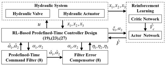
Figure 2. Structure of the Proposed RL-Based Predefined-Time Control Strategy.

3.4. Main Result and Stability Analysis

Theorem 1.

Consider the electro-hydraulic servo system model described by (5), which contains unknown dynamics and disturbances. Under Assumptions 1 and 2, if the control law is implemented according to (27), then the system tracking error converges to a bounded set within a predefined time, and all internal signals remain bounded.

Proof of Theorem 1.

By incorporating the predefined-time filter, the proof of tracking error convergence is transformed into demonstrating the convergence of a composite signal comprising both the filtered error compensation signal and its compensator. To proceed with the analysis, a new Lyapunov function is constructed as follows:

$$V_{\eta }=\frac{1}{2}{{\eta }_1}^2+\frac{1}{2}{{\eta }_2}^2+\frac{1}{2}{{\eta }_3}^2$$

(28)

The following inequality is established based on Lemma 3 in [31]:

$${\eta }_i({\widehat{\alpha }}_i-{\alpha }_i)\le |{\eta }_i||{\widehat{\alpha }}_i-{\alpha }_i|\le {\chi }_i|{\eta }_i|\le 3^{\frac{r}{2}}\frac{a_2}{r{T}_f{a}^{\prime }}{(\frac{1}{2}{{\eta }_i}^2)}^{1+\frac{r}{2}}+\frac{(1+r){\chi }_i}{2+r}{(\frac{(2+r)a_2}{2^{1+\frac{r}{2}}{\chi }_{i}r{T}_f{a}^{\prime }})}^{-\frac{1}{1+r}}$$

(29)

where the variable i = 1, 2, and the constant ${\chi }_i$ satisfies ${\chi }_i\ge |{\widehat{\alpha }}_i-{\alpha }_i|$.

Differentiating Equation (28) with respect to time yields:

$$\begin{array}{c}{\dot{V}}_{\eta }\le {\displaystyle \sum _{i=1}^2}\left[\begin{array}{l}{3}^{\frac{r}{2}}\frac{a_2}{r{T}_f{a}^{\prime }}{(\frac{1}{2}{{\eta }_i}^2)}^{1+\frac{r}{2}}+\frac{(1+r){\chi }_i}{2+r}{(\frac{(2+r)a_2}{2^{1+\frac{r}{2}}{\chi }_{i}r{T}_f{a}^{\prime }})}^{-\frac{1}{1+r}}\\ -\frac{1}{2}\cdot \frac{4}{r{T}_f}{{\eta }_i}^2-\frac{2a_1}{r{T}_f{a}^{\prime }}{(\frac{1}{2}{{\eta }_i}^2)}^{1-\frac{\gamma }{2}}-3^{\frac{r}{2}}\frac{3a_2}{r{T}_f{a}^{\prime }}{(\frac{1}{2}{{\eta }^2}_i)}^{1+\frac{\gamma }{2}}\end{array}\right]\\ -\frac{1}{2}\cdot \frac{4}{r{T}_f}{{\eta }_3}^2-\frac{2a_1}{r{T}_f{a}^{\prime }}{(\frac{1}{2}{{\eta }_3}^2)}^{1-\frac{\gamma }{2}}-3^{\frac{r}{2}}\frac{2a_2}{r{T}_f{a}^{\prime }}{(\frac{1}{2}{{\eta }^2}_3)}^{1+\frac{\gamma }{2}}+\frac{3r}{2-r}{\lambda }_{f12}\\ \le -\frac{2}{r{T}_f{a}^{\prime }}(2a^{\prime }{V}_{\eta }+a_1{V_{\eta }}^{1-\frac{r}{2}}+a_2{V_{\eta }}^{1+\frac{r}{2}})+M\end{array}$$

(30)

where the constant $M={\displaystyle \sum _{i=1}^2}[\frac{(1+r){\chi }_i}{2+r}{(\frac{(2+r)a_2}{2^{1+\frac{r}{2}}{\chi }_{i}r{T}_f{a}^{\prime }})}^{-\frac{1}{1+r}}]+\frac{3r}{2-r}{\lambda }_{f12}$. Then, according to Lemma 1, it is rigorously derived that the designed filter error compensator ${\eta }_i$ of the system achieves bounded convergence within a predefined time.

For the convergence proof of the filtered error compensation signal, the following Lyapunov function is constructed:

$$V_{\xi }=\frac{1}{2}{{\xi }_1}^2+\frac{1}{2}{{\xi }_2}^2+\frac{1}{2}{{\xi }_3}^2+\frac{1}{2{\delta }_c}{{\tilde{W}}_c}^T{\tilde{W}}_c+\frac{1}{2{\delta }_a}{{\tilde{W}}_a}^T{\tilde{W}}_a$$

(31)

Differentiating Equation (31) with respect to time yields:

$$\begin{array}{c}{\dot{V}}_{\xi }\le {\displaystyle \sum _{h=1}^3}(-{\lambda }_{eh1}{{\xi }_h}^2-{\lambda }_{eh2}{({{\xi }_h}^2)}^{1+\frac{\gamma }{2}}+\frac{1}{2}{{\lambda }_{\eta h1}}^2+\frac{1}{2}{{\lambda }_{\eta h2}}^2)\\ +{\xi }_2(-{{\tilde{W}}_a}^T{\phi }_a+{\epsilon }_a)+{\xi }_{3}d+\frac{1}{{\delta }_a}{{\tilde{W}}_c}^T{\dot{\widehat{W}}}_c+\frac{1}{{\delta }_a}{{\tilde{W}}_a}^T{\dot{\widehat{W}}}_a\end{array}$$

(32)

Given that ${\sigma }_1$ is bounded above by $-{{\tilde{W}}_a}^T{\phi }_a+{\epsilon }_a$, and ${\sigma }_2$ is bounded above by $d$. Furthermore, according to the mapping defined in Equation (18), the analytical result indicates that when conditions $||{\widehat{W}}_c||<||{\overline{W}}_c|| or ||{\widehat{W}}_c||=||{\overline{W}}_c||,{{\widehat{W}}_c}^T(h(t)+{{\widehat{W}}_c}^T\mathrm{\Lambda })\mathrm{\Lambda }>0$ and $||{\widehat{W}}_a||<||{\overline{W}}_a|| or ||{\widehat{W}}_a||=||{\overline{W}}_a||,{{\widehat{W}}_a}^T{\rho }_a>0$ are simultaneously satisfied, the additional constant S attains its maximum value. Therefore, stability verification under this maximal case directly ensures its general validity:

$$\begin{array}{l} \frac{1}{{\delta }_a}{{\tilde{W}}_c}^T{\dot{\widehat{W}}}_c+\frac{1}{{\delta }_a}{{\tilde{W}}_a}^T{\dot{\widehat{W}}}_a\\ \le -{{\tilde{W}}_c}^T(h(t)+{{\widehat{W}}_c}^T\mathrm{\Lambda })\mathrm{\Lambda }-{{\tilde{W}}_a}^T(K_V{\widehat{V}}_c({\xi }_1)+{{\tilde{W}}_a}^T{\phi }_a(X_a)-{\epsilon }_a){\phi }_a(X_a)\\ \le -{{\tilde{W}}_c}^T(-{W_c}^T\mathrm{\Lambda }+\varpi +{{\widehat{W}}_c}^T\mathrm{\Lambda })\mathrm{\Lambda }-K_V{{\tilde{W}}_a}^T{\phi }_a(X_a){{\widehat{W}}_c}^T{\phi }_c({\xi }_1)-{({{\tilde{W}}_a}^T{\phi }_a(X_a))}^2+{\epsilon }_a{{\tilde{W}}_a}^T{\phi }_a(X_a)\\ \le \frac{1}{2}{\lambda }_{\min }(\mathrm{\Lambda }{\mathrm{\Lambda }}^T)||W_c+{\overline{W}}_c|{|}^2+\frac{1}{2}{\varpi }^2+\frac{1}{2}{{\epsilon }_a}^2+({K_V}^2+\frac{1}{2}){\lambda }_{\min }({\phi }_a(X_a){\phi }_a{(X_a)}^T))||W_a+{\overline{W}}_a|{|}^2\\ +\frac{1}{4}{\lambda }_{\min }({\phi }_c({\xi }_1){\phi }_c{({\xi }_1)}^T)||{\overline{W}}_c|{|}^2\\ =N\end{array}$$

(33)

Since N is a bounded constant, Equation (32) can be further simplified to:

$$\begin{array}{l}{\dot{V}}_{\xi }\le -\frac{2}{r{T}_f{a}^{\prime }}(2a^{\prime }{V}_{\xi }+a_1{V_{\xi }}^{1-\frac{r}{2}}+a_2{V_{\xi }}^{1+\frac{r}{2}})+{\displaystyle \sum _{h=1}^3}(\frac{1}{2}{{\lambda }_{\eta h1}}^2+\frac{1}{2}{{\lambda }_{\eta h2}}^2+\frac{r}{2-r}{\lambda }_{e12})+\frac{1}{2}{{\sigma }_1}^2\\ +\frac{1}{2}{{\sigma }_2}^2+N+\frac{2}{r{T}_f{a}^{\prime }}(2a^{\prime }||W_c+{\overline{W}}_c|{|}^2+a_1{(||W_c+{\overline{W}}_c|{|}^2)}^{1-\frac{r}{2}}+a_2{(||W_c+{\overline{W}}_c|{|}^2)}^{1+\frac{r}{2}})\\ +\frac{2}{r{T}_f{a}^{\prime }}(2a^{\prime }||W_a+{\overline{W}}_a|{|}^2+a_1{(||W_a+{\overline{W}}_a|{|}^2)}^{1-\frac{r}{2}}+a_2{(||W_a+{\overline{W}}_a|{|}^2)}^{1+\frac{r}{2}})\end{array}$$

(34)

where the constant ${\lambda }_{e12}=\frac{2-r}{2}{(\frac{1}{2})}^{1-\frac{r}{2}}\cdot \frac{2a_1}{r{T}_f{a}^{\prime }}$.

Recalling Lemma 1, it is derived that the filtered error compensation signal ${\xi }_i$ exhibits predefined-time boundedness. Since $e_1={\xi }_1+{\eta }_1$ holds, the system tracking error is consequently guaranteed to achieve bounded stability after the predefined time, thereby completing the proof. □

Remark 2.

In practical implementations, raw sensor signals are commonly pre-filtered (e.g., second- or third-order filters) to attenuate high-frequency noise before being used by the control algorithm. Beyond this standard pre-processing, the proposed control architecture itself incorporates several inherent mechanisms that further suppress residual measurement noise: (i) the predefined-time backstepping core exhibits low-pass closed-loop dynamics, naturally attenuating high-frequency components in the feedback path; (ii) the non-singular predefined-time command filter smooths the error-signal sequence, adding a further barrier to noise propagation in the recursive design; and (iii) the Actor–Critic RL updates are intrinsically insensitive to zero-mean high-frequency noise, so that the resulting compensation signal remains smooth.

Remark 3.

Since the RL network has been proven to work without boundedness assumptions in the mechanical channel, a natural extension would be to design an RL network to learn and compensate for the uncertainties in the hydraulic dynamics. However, a core challenge in the current RL design scheme is the practical difficulty in reliably obtaining accurate differential signals of the pressure dynamics. Therefore, a promising future direction is to replace the model-based backstepping control with a reinforcement learning framework for controller design, so that it outputs the optimal control law directly—rather than just using RL to compensate for uncertainties.

4. Simulation Results

The simulations in this study were conducted with MATLAB R2018a.

To validate the efficacy of the proposed reinforcement learning-based predefined-time tracking controller, this section provides a comprehensive evaluation through comparative simulations of the electro-hydraulic servo system model under different control schemes. The system parameters are specified as follows: m = 30 kg, A = 904.8 mm², B_v = 4000 N·s/m, V_t = 7.96 × 10⁻⁵ m³, k_u = 1.197 × 10⁻⁸ m³/s/V/Pa^1/2, P_s = 10 MPa, β_e = 700 MPa, and C_t = 1 × 10⁻¹³ m³/s/Pa. The intermediate variable F is set as $F=B_v{x}_2/m$.

The desired trajectory for the system is specified as 0.01·cos(2·t) m. For comparative analysis, the following controllers are implemented:

(1) RLPDTC: The proposed RL-based predefined-time controller for electro-hydraulic servo systems. The basic parameters are configured as: r = 0.2, ζ = 1, η = 0.001, κ = 100, λ = 0.5, a₁ = 50, a₂ = 1, and T_f = 1 s.

(2) PDTC: A predefined-time controller without reinforcement learning-based dynamic compensation. All parameters remain identical to RLPDTC to specifically evaluate the contribution of the RL-based active compensation.

(3) VFPI: A velocity feed-forward PI controller with the structure $u=k_P{z}_1+k_I\int z_{1}dt+k_F{\dot{x}}_{1d}$, where $z_1=x_{1d}-x_1$ denotes the tracking error. The parameters are set as: k_p = 150 (proportional gain), k_i = 30 (integral gain), and k_F = 20 (velocity feed-forward coefficient).

Remark 4.

Based on the structure of the actor and critic neural networks given from Equation (9) to Equation (15), the key structural parameters of the proposed RLPDTC are designed as follows. The number of hidden-layer neurons $v$ for both the actor and critic networks is set to 5. This value was determined through simulation trial-and-error and existing control research experience, which helps avoid overfitting when approximating the unknown nonlinear dynamics F. The activation function is chosen as the Gaussian function, as shown in reference [28], to ensure numerical stability during the learning process. Weight initialization with small random values is a common practice in adaptive control, which prevents excessively large initial control signals and ensures a smooth start to the learning process. The selection of the learning rate among the weight update gain parameters is based on stability considerations of the gradient descent method—too large a value can cause oscillations, while too small a value leads to slow convergence. Through tuning, we chose ${\delta }_c=1$ and ${\delta }_a=200$, which maintains system stability while ensuring a satisfactory convergence rate. The discount factor $\upsilon$ is set to 0.05 to balance the importance of immediate and future rewards. A smaller value promotes a faster system response, making it more suitable for short-term, highly dynamic tasks. The gain parameter $K_V=0.08$ was selected through simulation tuning, balancing convergence speed and approximation capability via a trial-and-error approach.

Figure 3 and Figure 4, respectively, show the comparative position tracking errors of the electro-hydraulic servo system under RLPDTC, PDTC, and VFPI control, along with the output tracking performance of RLPDTC following the desired command. As clearly demonstrated in Figure 3, RLPDTC exhibits enhanced compensation capability for unknown system dynamics compared to both PDTC and VFPI, leading to improved transient convergence performance. Moreover, the steady-state tracking error achieved by RLPDTC is significantly smaller, with the error amplitude ultimately stabilizing at 0.04 mm. By incorporating the reinforcement learning-based dynamic compensation mechanism into the predefined-time intelligent control design, RLPDTC ensures that the tracking error converges to a bounded range within the predefined time, thereby substantially enhancing tracking performance. The results confirm that RLPDTC achieves superior control effectiveness when compared with both PDTC and VFPI controllers. To quantitatively evaluate the performance of the RLPDTC and PDTC, the performance comparison for the last cycle is presented in the table below, where the maximum, average, and standard deviation of the tracking error are denoted as Me, μ, and σ, respectively. According to Table 1, RLPDTC reduces the maximum tracking error by approximately 81% and the mean square error by about 82%, demonstrating that the proposed method substantially improves tracking control accuracy and operational smoothness.

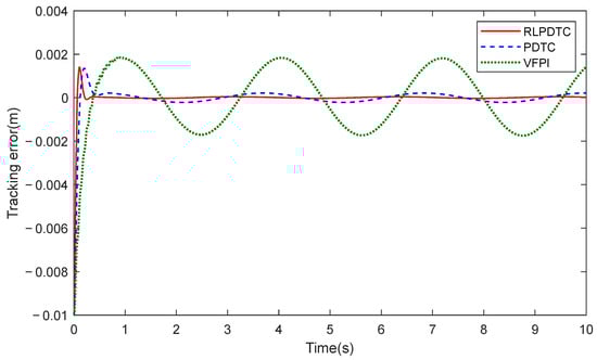
Figure 3. Comparison of tracking errors.

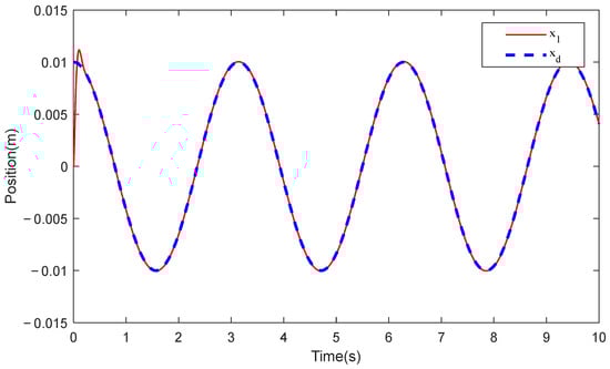
Figure 4. Tracking performance of RLPDTC.

Table 1. Performance indices of the last one cycle.

Indices	Me	μ	σ
RLPDTC	3.9461 × 10−5	2.5966 × 10−6	2.6262 × 10−5
PDTC	2.1107 × 10−4	2.6383 × 10−6	1.4840 × 10−4

Furthermore, Figure 5 illustrates the approximation performance of RLPDTC for the system’s unknown dynamics, while Figure 6 and Figure 7 present the temporal evolution of the reinforcement learning network weights. The results demonstrate RLPDTC’s superior capability in accurately estimating unknown system dynamics, thereby verifying the efficacy of the integrated reinforcement learning-based compensation mechanism. Figure 8 displays the control input trajectory generated by the proposed RLPDTC framework. The obtained control signal exhibits smooth and continuous characteristics, confirming its practical applicability for real-world implementation.

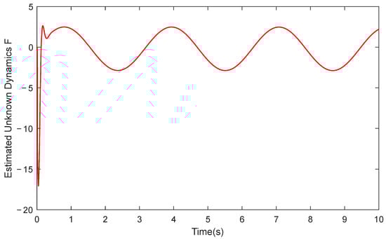
Figure 5. Estimated Unknown Dynamics of RLPDTC.

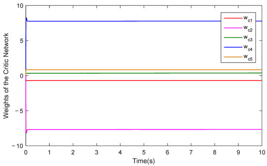
Figure 6. Critic network weights of RLPDTC.

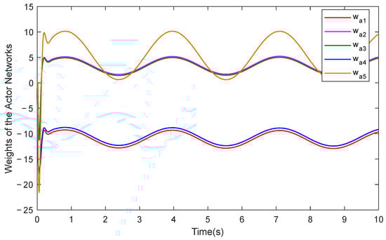
Figure 7. Actor network weights of RLPDTC.

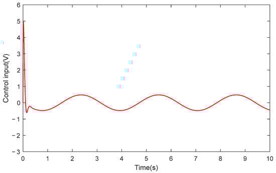
Figure 8. Control input signal of RLPDTC.

An explicit high-frequency sinusoidal disturbance, sin(10t), whose frequency is significantly higher than the system’s main dynamic bandwidth, was superimposed on the original uncertainty F to simulate a type of high-frequency uncertainty. As shown in Figure 9, the Actor–Critic network demonstrates a considerable ability to approximate this high-frequency disturbance. This confirms that, within the simulation environment, our intelligent compensation mechanism also possesses adaptability to uncertainties that change relatively quickly. As shown in Figure 10, after introducing these high-frequency uncertainties, the tracking error exhibits the expected, minor high-frequency fluctuations, but their amplitude is strictly confined within an acceptable engineering range. Importantly, the predefined-time convergence property is not compromised, and the global stability of the system is maintained. This result verifies the robustness of the proposed framework against specific high-frequency uncertainties.

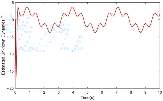
Figure 9. High-frequency uncertainties: estimation of RLPDTC.

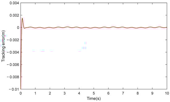
Figure 10. Tracking Error of RLPDTC Under High-frequency Uncertainty.

5. Conclusions

This paper proposes a novel predefined-time intelligent control framework for electro-hydraulic servo systems. By integrating a reinforcement learning strategy into the predefined-time backstepping design, the controller is capable of approximating and actively feedforward-compensating for unmodeled system dynamics. Consequently, the system exhibits significant robustness without requiring prior knowledge of uncertainty bounds, and the key compensation effect is verified in comparative simulations. Within the novel predefined-time control framework, the system convergence time can be explicitly specified by the user and remains independent of the initial system conditions. This is rigorously supported by stability proofs and simulation validations. Simulation results demonstrate that the proposed method achieves superior tracking accuracy and convergence speed compared to existing representative control methods. This study also acknowledges its limitations, as the controller design still relies noticeably on key system parameter information. Therefore, future work will focus on enhancing the intelligence of hydraulic control systems, specifically in terms of self-tuning control parameters and optimizing the controller design.

References

- Mattila, J.; Koivumaki, J.; Caldwell, D.G.; Semini, C. A survey on control of hydraulic robotic manipulators with projection to future trends. IEEE/ASME Trans. Mechatron. 2017, 22, 669–680. [Google Scholar] [CrossRef]
- Guo, Q.; Chen, Z. Neural adaptive control of single-rod electrohydraulic system with lumped uncertainty. Mech. Syst. Signal Process. 2021, 146, 106869. [Google Scholar] [CrossRef]
- Huang, Y.; Na, J.; Wu, X.; Gao, G. Approximation-free control for vehicle active suspensions with hydraulic actuator. IEEE Trans. Ind. Electron. 2018, 65, 7258–7267. [Google Scholar] [CrossRef]
- Liu, X.; Liu, W.; Zhou, C.; Huang, M. Probabilistic weighted support vector machine for robust modeling with application to hydraulic actuator. IEEE Trans. Ind. Inform. 2017, 13, 1723–1733. [Google Scholar] [CrossRef]
- Fallahi, M.; Zareinejad, M.; Baghestan, K.; Tivay, A.; Rezaei, S.M.; Abdullah, A. Precise position control of an electro-hydraulic servo system via robust linear approximation. ISA Trans. 2018, 80, 503–512. [Google Scholar] [CrossRef]
- Lu, K.; Feng, G.; Ding, B. Robust H-Infinity Tracking Control for a Valve-Controlled Hydraulic Motor System with Uncertain Parameters in the Complex Load Environment. Sensors 2023, 23, 9092. [Google Scholar] [CrossRef]
- Chen, C.-Y.; Li, T.-H.S.; Yeh, Y.-C.; Chang, C.-C. Design and implementation of an adaptive sliding-mode dynamic controller for wheeled mobile robots. Mechatronics 2009, 19, 156–166. [Google Scholar] [CrossRef]
- Yao, J.; Jiao, Z.; Yao, B. Robust control for static loading of electro-hydraulic load simulator with friction compensation. Chin. J. Aeronaut. 2012, 25, 954–962. [Google Scholar] [CrossRef]
- Zhou, J.; Hua, C.; Zhang, B.; Li, Y.; Zhang, Y. Performance Guaranteed Robust Tracking Control of Electro-Hydraulic Systems with Input Delays and Output Constraints. IEEE Trans. Ind. Electron. 2025, 72, 14469–14477. [Google Scholar] [CrossRef]
- Wang, S.; Na, J.; Ren, X. RISE-based asymptotic prescribed performance tracking control of nonlinear servo mechanisms. IEEE Trans. Syst. Man Cybern. Syst. 2018, 48, 2359–2370. [Google Scholar] [CrossRef]
- Liu, L.; Yue, X.; Wen, H.; Dai, H. RISE-based adaptive tracking control for Euler-Lagrange mechanical systems with matched disturbances. ISA Trans. 2023, 135, 94–104. [Google Scholar] [CrossRef]
- Cao, H.; Li, Y.; Liu, C.; Zhao, S. ESO-based robust and high-precision tracking control for aerial manipulation. IEEE Trans. Autom. Sci. Eng. 2023, 21, 2139–2155. [Google Scholar] [CrossRef]
- Tang, G.; Xue, W.; Huang, X.; Song, K. On error-driven nonlinear ESO based control design with application to air-fuel ratio control of engines. Control Eng. Pract. 2024, 143, 105808. [Google Scholar] [CrossRef]
- Xu, B.; Zhang, L.; Ji, W. Improved non-singular fast terminal sliding mode control with disturbance observer for PMSM drives. IEEE Trans. Transp. Electrif. 2021, 7, 2753–2762. [Google Scholar] [CrossRef]
- Wei, X.; Song, X.; Zhang, H.; Hu, X.; Li, X. Disturbance-observer-based tracking trajectory control of under-actuated surface vessel with input and output constraints. Appl. Math. Model. 2026, 153, 116598. [Google Scholar] [CrossRef]
- Ma, J.; Yao, Z.; Deng, W.; Yao, J. Fixed-time adaptive neural network compensation control for uncertain nonlinear systems. Neural Netw. 2025, 189, 107563. [Google Scholar] [CrossRef]
- Kharrat, M. Neural networks-based adaptive fault-tolerant control for stochastic nonlinear systems with unknown backlash-like hysteresis and actuator faults. J. Appl. Math. Comput. 2024, 70, 1995–2018. [Google Scholar] [CrossRef]
- Ma, B.; Liu, Z.; Zhao, W.; Yuan, J.; Long, H.; Wang, X.; Yuan, Z. Target tracking control of UAV through deep reinforcement learning. IEEE Trans. Intell. Transp. Syst. 2023, 24, 5983–6000. [Google Scholar] [CrossRef]
- Bai, W.; Chen, D.; Zhao, B.; D’Ariano, A. Reinforcement learning control for a class of discrete-time non-strict feedback multi-agent systems and application to multi-marine vehicles. IEEE Trans. Intell. Veh. 2024, 10, 3613–3625. [Google Scholar] [CrossRef]
- Wang, N.; Gao, Y.; Zhao, H.; Ahn, C.K. Reinforcement learning-based optimal tracking control of an unknown unmanned surface vehicle. IEEE Trans. Neural Netw. Learn. Syst. 2020, 32, 3034–3045. [Google Scholar] [CrossRef] [PubMed]
- Zheng, M.; Wu, Y.; Li, C. Reinforcement learning strategy for spacecraft attitude hyperagile tracking control with uncertainties. Aerosp. Sci. Technol. 2021, 119, 107126. [Google Scholar] [CrossRef]
- Liang, X.; Yao, Z.; Ge, Y.; Yao, J. Disturbance observer based actor-critic learning control for uncertain nonlinear systems. Chin. J. Aeronaut. 2023, 36, 271–280. [Google Scholar] [CrossRef]
- Yao, Z.; Liang, X.; Jiang, G.-P.; Yao, J. Model-based reinforcement learning control of electrohydraulic position servo systems. IEEE/ASME Trans. Mechatron. 2022, 28, 1446–1455. [Google Scholar] [CrossRef]
- Chen, J.; Du, X.; Lyu, L.; Fei, Z.; Sun, X.-M. Accurate Finite-Time Motion Control of Hydraulic Actuators with Event-Triggered Input. IEEE Trans. Autom. Sci. Eng. 2024, 21, 5826–5836. [Google Scholar] [CrossRef]
- Liang, X.; Yao, Z.; Deng, W.; Yao, J. Adaptive neural network finite-time tracking control for uncertain hydraulic manipulators. IEEE/ASME Trans. Mechatron. 2024, 30, 645–656. [Google Scholar] [CrossRef]
- Wang, C.; Wang, J.; Guo, Q.; Liu, Z.; Chen, C.L.P. Disturbance Observer-Based Fixed-Time Event-Triggered Control for Networked Electro-Hydraulic Systems with Input Saturation. IEEE Trans. Ind. Electron. 2025, 72, 1784–1794. [Google Scholar] [CrossRef]
- Chen, R.-Z.; Li, Y.-X.; Ahn, C.K. Reinforcement-learning-based fixed-time attitude consensus control for multiple spacecraft systems with model uncertainties. Aerosp. Sci. Technol. 2023, 132, 108060. [Google Scholar] [CrossRef]
- Cao, S.; Sun, L.; Jiang, J.; Zuo, Z. Reinforcement learning-based fixed-time trajectory tracking control for uncertain robotic manipulators with input saturation. IEEE Trans. Neural Netw. Learn. Syst. 2021, 34, 4584–4595. [Google Scholar] [CrossRef]
- Sánchez-Torres, J.D.; Gómez-Gutiérrez, D.; López, E.; Loukianov, A.G. A class of predefined-time stable dynamical systems. IMA J. Math. Control Inf. 2018, 35, i1–i29. [Google Scholar] [CrossRef]
- Xie, S.; Chen, Q. Predefined-Time Disturbance Estimation and Attitude Control for Rigid Spacecraft. IEEE Trans. Circuits Syst. II Express Briefs 2024, 71, 2089–2093. [Google Scholar] [CrossRef]
- Que, N.; Sun, H.; Deng, W.; Yao, J.; Zhao, X.; Hu, J.; Luo, M. Command Filter-Based Adaptive Predefined-Time Tracking Control for Uncertain Systems with Disturbance Compensation. Int. J. Robust Nonlinear Control 2025, 35, 6604–6618. [Google Scholar] [CrossRef]
Disclaimer/Publisher’s Note: The statements, opinions and data contained in all publications are solely those of the individual author(s) and contributor(s) and not of MDPI and/or the editor(s). MDPI and/or the editor(s) disclaim responsibility for any injury to people or property resulting from any ideas, methods, instructions or products referred to in the content. |
© 2025 by the authors. Licensee MDPI, Basel, Switzerland. This article is an open access article distributed under the terms and conditions of the Creative Commons Attribution (CC BY) license.