Event-Triggered Control for Discrete-Time Linear Systems Under Actuator and Sensor Constraints

Abstract

This paper focuses on designing an event-triggered dynamic output feedback controller for discrete-time linear systems subject to actuator and sensor constraints as well as external disturbances. A dynamic event-triggered condition with two generalized weighting parameters is introduced to regulate sensor-to-controller communication. By integrating generalized sector conditions, Lyapunov analysis, and linearization techniques, sufficient conditions are derived in terms of linear matrix inequalities, ensuring bounded closed-loop trajectories, prescribed $H_{\infty }$ performance, and asymptotic stability in the disturbance-free case. Furthermore, optimization problems are formulated to maximize the event-triggering rate while preserving the desired system performance. Simulation results show that, compared to time-triggered control, the event-triggered control effectively reduces the communication frequency, thereby significantly conserving communication resources. Compared with existing results, this work presents the first event-triggered dynamic output feedback scheme for discrete-time linear systems with dual saturation constraints. The inclusion of generalized weighting parameters and the use of generalized sector conditions allow the design to be carried out within a flexible local framework with reduced conservatism.

1. Introduction

Actuator saturation, inherent in nearly all feedback control systems due to physical limitations, introduces nonlinear behavior that can severely degrade performance and potentially destabilize the system [1,2,3,4,5]. Designing effective controllers for such systems requires explicitly accounting for these saturation constraints during stability analysis and synthesis. Common design approaches are performed within either the global/semi-global framework or the local framework [6,7,8]. For exponentially unstable open-loop systems, controller design is typically conducted within a regional framework. Within this framework, two principal methodologies have been established to address saturation nonlinearities: polytopic model representations [7,9] and modified sector conditions [6,10].

Sensor saturation represents another prevalent nonlinearity in control systems, arising when sensors reach their physical measurement limits. This phenomenon distorts output signals, yielding incomplete or erroneous controller feedback. Similar to actuator saturation, sensor saturation degrades stability margins and can potentially lead to system instability if unaddressed. Over past decades, substantial research efforts have addressed under sensor saturation constraints [11,12,13]. In particular, significant advances in controller synthesis have been achieved in [14,15] through explicit consideration of concurrent actuator and sensor saturations. This co-design approach acknowledges the coupled nature of dual saturation effects and their collective impact on overall system performance and stability.

Networked control systems (NCSs) constitute feedback control loops wherein sensors, controllers, and actuators communicate via a shared digital network, replacing traditional point-to-point connections. This structure offers significant advantages, including reduced wiring complexity, enhanced system flexibility, and simplified maintenance [16,17,18]. However, it introduces inherent challenges such as network-induced delays, data packet dropouts, limited bandwidth, and scheduling constraints [19,20,21,22,23]. To efficiently manage communication resource utilization while preserving desired system performance, event-triggered mechanisms (ETMs) have been developed, under which sensor data transmissions occur only when specific triggering conditions are violated, significantly reducing network resource usage [24,25,26,27]. Consequently, substantial analysis and synthesis frameworks have been sufficiently established for NCSs employing ETMs [28,29,30,31,32].

Over the past decade, significant advances have emerged for NCSs incorporating saturation constraints [33,34,35], with recent studies increasingly employed ETMs to address these challenges [36,37,38,39,40,41,42]. For instance, a static ETM has been utilized to solve the dynamic output feedback control problem for discrete-time LPV systems with actuator constraints [41]. The $H_{\infty }$ control problem has been examined for singularly perturbed systems subject to time delays and sensor saturations under a dynamic ETM [39]. Notably, concurrent sensor and actuator saturations have been tackled in designing the event-triggered dynamic output-feedback controller [43]. However, two limitations persist in existing research: (1) current dual-saturation treatments in [43] rely on non-strict inequalities rather than rigorous generalized sector-bound conditions; and (2) the results in [43] are exclusively confined to continuous-time domains, leaving discrete-time formulations underdeveloped.

To bridge the aforementioned gaps, this paper develops a novel event-triggered control framework for discrete-time systems simultaneously subject to actuator saturation, sensor saturation, and external disturbances. The main contributions are summarized as follows. (1) A unified co-design procedure is established for the dynamic output-feedback controller and the ETM. Furthermore, optimization problems are formulated to maximize the event-triggering rate (ETR), thereby explicitly balancing communication efficiency with prescribed control performance. (2) Unlike the approach in [39], two generalized weighting parameters are introduced in the event-triggering condition (ETC), which allows the derivation of LMI conditions without resorting to conservative bounding inequalities, thus reducing design conservatism. (3) In contrast to the continuous-time method in [43] that relies on non-strict inequalities, a discrete-time formulation is developed. It rigorously handles actuator and sensor saturations using generalized sector-bound conditions within a local framework, offering a more systematic and less conservative treatment for discrete-time NCSs.

Notation. ${\mathbb{R}}^n$: n-dimensional Euclidean space; $P>0(\ge 0)$: the symmetric and positive definite (positive semi-definite) matrix; I: the identity matrix of suitable dimension.

2. Problem Formulation

Consider the discrete-time linear system

$$\hfill \left\{\begin{array}{c}x(k+1)=Ax\left(k\right)+B{\mathrm{sat}}_u\left(u\right(k\left)\right)+B_{w}w\left(k\right),\hfill \\ y\left(k\right)={\mathrm{sat}}_y\left(Cx\right(k\left)\right),z\left(k\right)=C_{z}x\left(k\right),\hfill \end{array}\right.$$

(1)

where $x\left(k\right)\in {\mathbb{R}}^n$ is the system state, $u\left(k\right)\in {\mathbb{R}}^m$ is the control input, $y\left(k\right)\in {\mathbb{R}}^p$ is the measurement output, $z\left(k\right)\in {\mathbb{R}}^q$ is the controlled output, $w\left(k\right)\in {\mathbb{R}}^r$ is the disturbance input, A, B, $B_w$, C and $C_z$ are known constant matrices. The functions ${\mathrm{sat}}_u\left(u\right)=\mathrm{col}\{{\mathrm{sat}}_u\left(u_1\right),{\mathrm{sat}}_u\left(u_2\right),\dots ,{\mathrm{sat}}_u\left(u_m\right)\}$ and ${\mathrm{sat}}_y\left(y\right)=\mathrm{col}\{{\mathrm{sat}}_y\left(y_1\right),{\mathrm{sat}}_y\left(y_2\right),\dots ,{\mathrm{sat}}_y\left(y_p\right)\}$ represent actuator and sensor constraints, respectively, where

$$\begin{array}{cc}\hfill {\mathrm{sat}}_u\left(u_i\right)& =\mathrm{sign}\left(u_i\right)\min \{{\overline{u}}_i,|u_i\left|\right\},i=1,2,\dots ,m,\hfill \\ \hfill {\mathrm{sat}}_y\left(y_j\right)& =\mathrm{sign}\left(y_j\right)\min \{{\overline{y}}_j,|y_j\left|\right\},j=1,2,\dots ,p.\hfill \end{array}$$

Here, ${\overline{u}}_i$ and ${\overline{y}}_j$ denote the saturation levels.

In addition, the disturbance $w\left(k\right)$ is assumed to satisfy

$$\begin{array}{c}\hfill \sum _{k=0}^{+\infty }{w}^T\left(k\right)w\left(k\right)\le \delta ,\delta >0.\end{array}$$

(2)

In this paper, output signals are assumed to be transmitted through communication networks. To conserve communication resources, the ETM is employed. The triggering instants are denoted by $k_s$$(s=0,1,2,\dots )$, determined by the following ETC:

$$\begin{array}{cc}\hfill k_{s+1}=& \underset{k\in N}{\min }\{k|k>k_s,{\displaystyle \frac{1}{\vartheta }}\mu \left(k\right)+y^T\left(k\right){\Omega }_{y}y\left(k\right)-e^T\left(k\right){\Omega }_{e}e\left(k\right)\le 0\},k_0=0\hfill \end{array}$$

(3)

where $e\left(k\right)\triangleq y\left(k_s\right)-y\left(k\right)$, $\vartheta >0$ is a given scalar, ${\Omega }_y>0$, ${\Omega }_e>0$ are two matrices to be designed. The variable $\mu \left(k\right)$ in (3) evolves according to the dynamic equation

$$\begin{array}{c}\hfill \mu (k+1)=\lambda \mu \left(k\right)+y^T\left(k\right){\Omega }_{y}y\left(k\right)-e^T\left(k\right){\Omega }_{e}e\left(k\right)\end{array}$$

(4)

with initial condition $\mu \left(0\right)\ge 0$ and parameter $0<\lambda <1$.

Remark  1.

The triggering instants $k_s$$(s=0,1,2,\dots )$ are determined by the ETC (3) together with the Equation (4). The weighting parameters ${\Omega }_y$ and ${\Omega }_e$ in (3) and (4) can be obtained directly by solving the subsequent LMI-based optimization problems for given scalars $0<\lambda <1$ and $\vartheta >0$.

This paper focuses on designing an event-triggered dynamic output feedback controller with an anti-windup term:

$$\begin{array}{c}\hfill \left\{\begin{array}{c}{x}_c(k+1)=A_c{x}_c\left(k\right)+B_{c}y\left(k_l\right)+E_c({\mathrm{sat}}_u\left(u\left(k\right)\right)-u\left(k\right)),\hfill \\ u\left(k\right)=C_c{x}_c\left(k\right)+D_{c}y\left(k_s\right),t\in [k_s,k_{s+1}),s=0,1,2,\dots ,\hfill \end{array}\right.\end{array}$$

(5)

where $x_c\left(k\right)\in {\mathbb{R}}^{n_c}$ is the controller state, and $A_c$, $B_c$, $C_c$, $D_c$, $E_c$ are gain matrices.

Define the augmented state vector $\overline{x}\left(k\right)\triangleq \mathrm{col}\{x\left(k\right),x_c\left(k\right)\}$$\in {\mathbb{R}}^{\overline{n}}$ where $\overline{n}=n+n_c$, and introduce the following nonlinear terms:

$$\begin{array}{cc}\hfill {\phi }_u\left(k\right)\triangleq & {\mathrm{sat}}_u\left(u\left(k\right)\right)-u\left(k\right),{\phi }_y\left(k\right)\triangleq {\mathrm{sat}}_y\left(Cx\left(k\right)\right)-Cx\left(k\right).\hfill \end{array}$$

From (1) and (5), the closed-loop system is then given by

$$\begin{array}{c}\hfill \left\{\begin{array}{c}\overline{x}(k+1)=\overline{A}\overline{x}\left(k\right)+{\overline{B}}_u{\phi }_u\left(k\right)+{\overline{B}}_y{\phi }_y\left(k\right)\hfill \\ +{\overline{B}}_{y}e\left(k\right)+{\overline{B}}_{w}w\left(k\right),\hfill \\ y\left(k\right)={\overline{C}}_y\overline{x}\left(k\right)+{\phi }_y\left(k\right),z\left(k\right)={\overline{C}}_z\overline{x}\left(k\right),\hfill \\ u\left(k\right)={\overline{C}}_u\overline{x}\left(k\right)+D_c{\phi }_y\left(k\right)+D_{c}e\left(k\right),\hfill \end{array}\right.\end{array}$$

(6)

where

$$\begin{gathered} \overline{A}\triangleq \left[\begin{array}{cc}A+B{D}_{c}C\hfill & B{C}_c\\ B_{c}C& A_c\end{array}\right],{\overline{B}}_u\triangleq \left[\begin{array}{c}B\\ E_c\end{array}\right],{\overline{B}}_y\triangleq \left[\begin{array}{c}B{D}_c\\ B_c\end{array}\right], \\ {\overline{B}}_w\triangleq \left[\begin{array}{c}{B}_w\hfill \\ 0\end{array}\right],{\overline{C}}_y\triangleq \left[\begin{array}{cc}C& 0\end{array}\right],{\overline{C}}_z\triangleq \left[\begin{array}{cc}{C}_z& 0\end{array}\right],{\overline{C}}_u\triangleq \left[\begin{array}{cc}{D}_{c}C& C_c\end{array}\right]. \end{gathered}$$

Here, the initial conditions of the system (6) are denoted by ${\overline{x}}_0\triangleq \mathrm{col}\{x_0,x_{c0}\}$.

To address the nonlinear terms ${\phi }_y\left(k\right)$ and ${\phi }_u\left(k\right)$ in the system (6), we employ the modified sector conditions [6,10]. This requires the following two constraints:

$$\begin{array}{c}\hfill |v_i\left(k\right)|\le {\overline{u}}_i,i=1,2,\dots ,m,\end{array}$$

(7)

$$\begin{array}{c}\hfill |{\rho }_j\left(k\right)|\le {\overline{y}}_j,j=1,2,\dots ,p,\end{array}$$

(8)

where $v\left(k\right)=G_u\overline{x}\left(k\right)$, $\rho \left(k\right)=G_y\overline{x}\left(k\right)$, with $G_u$ and $G_y$ being $m\times \overline{n}$ and $p\times \overline{n}$ gain matrices, respectively. Then, for any $m\times m$ diagonal matrix $H_u>0$ and $p\times p$ diagonal matrix $H_y>0$, the following modified sector conditions hold [10]:

$$\begin{array}{cc}\hfill & -2{\phi }_u^T\left(k\right)H_u\left[{\phi }_u\left(k\right)+({\overline{C}}_u-G_u)\overline{x}\left(k\right)+D_c{\phi }_y\left(k\right)+D_{c}e\left(k\right)\right]\ge 0,\hfill \end{array}$$

(9)

$$\begin{array}{cc}\hfill & -2{\phi }_y^T\left(k\right)H_y\left[{\phi }_y\left(k\right)+({\overline{C}}_y-G_y)\overline{x}\left(k\right)\right]\ge 0.\hfill \end{array}$$

(10)

The main objectives of this paper are to design the event-triggered dynamic output feedback controller (5) that ensures the closed-loop system (6) exhibits: (1) bounded system states for all admissible initial conditions ${\overline{x}}_0$ and disturbances $w\left(k\right)$ satisfying (2); (2) satisfied $H_{\infty }$ performance requirement

$$\begin{array}{cc}\hfill & \sum _{k=0}^{+\infty }{z}^T\left(k\right)z\left(k\right)\le \gamma \sum _{k=0}^{+\infty }{w}^T\left(k\right)w\left(k\right)+\gamma V\left(0\right)(\gamma >0),\hfill \end{array}$$

(11)

where $V\left(k\right)$ denotes the Lyapunov function; (3) asymptotic stability in the absence of external disturbances ($w\left(k\right)\equiv 0$).

3. Main Results

To analyze the stability of the system (6), we consider the Lyapunov function

$$V\left(k\right)={\overline{x}}^T\left(k\right)P\overline{x}\left(k\right)+{\displaystyle \frac{1}{\vartheta }}\mu \left(k\right),P>0.$$

(12)

Theorem 1.

Given scalars $0<\lambda <1$ and $\vartheta >0$, suppose there exist $\overline{n}\times \overline{n}$ matrix $P>0$, $m\times \overline{n}$ matrix $G_u$, $p\times \overline{n}$ matrix $G_y$, $p\times p$ matrices ${\Omega }_y$, ${\Omega }_e$, $m\times m$ diagonal matrix $H_u>0$, $p\times p$ diagonal matrix $H_y>0$, and scalars $\delta >0$, $\gamma >0$, $\beta >0$ with $\beta \le 1/\delta$, such that

$$\begin{array}{cc}\hfill & \left[\begin{array}{cccc}{\Xi }_0& {\Xi }_1^T& {\Xi }_2^T& {\Xi }_3^T\\ \ast & -P& 0& 0\\ \ast & \ast & -\vartheta {\Omega }_y^{-1}& 0\\ \ast & \ast & \ast & -\gamma I\end{array}\right]<0,\hfill \end{array}$$

(13)

$$\begin{array}{cc}\hfill & \left[\begin{array}{cc}{\overline{u}}_i^2\beta & G_{ui}\\ \ast & P\end{array}\right]\ge 0,i=1,2,\dots ,m,\hfill \end{array}$$

(14)

$$\begin{array}{cc}\hfill & \left[\begin{array}{cc}{\overline{y}}_j^2\beta & G_{yj}\\ \ast & P\end{array}\right]\ge 0,j=1,2,\dots ,p,\hfill \end{array}$$

(15)

where $G_{ui}$ and $G_{yj}$ are the i-th row of the matrix $G_u$ and j-th row of the matrix $G_y$, respectively, and

$$\begin{array}{cc}\hfill {\Xi }_0=& \left[\begin{array}{cccccc}-P& {\Xi }_{12}& {\Xi }_{13}& 0& 0& 0\\ \ast & -2H_u& {\Xi }_{23}& {\Xi }_{24}& 0& 0\\ \ast & \ast & -2H_y& 0& 0& 0\\ \ast & \ast & \ast & {\Xi }_{44}& 0& 0\\ \ast & \ast & \ast & \ast & -I& 0\\ \ast & \ast & \ast & \ast & \ast & {\Xi }_{66}\end{array}\right],\hfill \\ \hfill {\Xi }_1=& \left[\begin{array}{cccccc}P\overline{A}& P{\overline{B}}_u& P{\overline{B}}_y& P{\overline{B}}_y& P{\overline{B}}_w& 0\end{array}\right],\hfill \\ \hfill {\Xi }_2=& \left[\begin{array}{cccccc}{\overline{C}}_y& 0& I& 0& 0& 0\end{array}\right],\hfill \\ \hfill {\Xi }_3=& \left[\begin{array}{cccccc}{\overline{C}}_z& 0& 0& 0& 0& 0\end{array}\right],\hfill \end{array}$$

with

$$\begin{array}{cc}\hfill {\Xi }_{12}& =(G_u^T-{\overline{C}}_u^T)H_u^T,{\Xi }_{13}=(G_y^T-{\overline{C}}_y^T)H_y^T,\hfill \\ \hfill {\Xi }_{23}& ={\Xi }_{24}=-H_u{D}_c,\hfill \\ \hfill {\Xi }_{44}& =-{\vartheta }^{-1}{\Omega }_e,{\Xi }_{66}={\vartheta }^{-1}(\lambda -1).\hfill \end{array}$$

Then: (1) The closed-loop system (6) has bounded trajectories for all ${\overline{x}}_0$ satisfying $V\left(0\right)\le 1/\beta -\delta$ and all disturbances satisfying (2); (2) The $H_{\infty }$ performance constraint (11) holds; (3) In the absence of disturbances, the asymptotic stability of system (6) is guaranteed for all ${\overline{x}}_0$ satisfying $V\left(0\right)\le 1/\beta$.

Proof. 

Denoting $\Delta V\left(k\right)\triangleq V(k+1)-V\left(k\right)$, and using Equations (4) and (6), inequalities (9) and (10), we obtain

$$\begin{gathered} \begin{array}{cc}\hfill & \Delta V\left(k\right)+(1/\gamma )z^T\left(k\right)z\left(k\right)-w^T\left(k\right)w\left(k\right)\hfill \\ \\ \hfill \le & {\overline{x}}^T(k+1)P\overline{x}(k+1)-{\overline{x}}^T\left(k\right)P\overline{x}\left(k\right)+[(\lambda -1)/\vartheta ]\mu \left(k\right)\hfill \\ \\ \hfill & -(1/\vartheta )e^T\left(k\right){\Omega }_{e}e\left(k\right)+(1/\vartheta ){[{\overline{C}}_y\overline{x}\left(k\right)+{\phi }_y\left(k\right)]}^T{\Omega }_y[{\overline{C}}_y\overline{x}\left(k\right)+{\phi }_y\left(k\right)]\hfill \\ \\ \hfill & -2{\phi }_u^T\left(k\right)H_u[{\phi }_u\left(k\right)+({\overline{C}}_u-G_u)\overline{x}\left(k\right)+D_c{\phi }_y\left(k\right)+D_{c}e\left(k\right)]\hfill \\ \\ \hfill & -2{\phi }_y^T\left(k\right)H_y\left[{\phi }_y\left(k\right)+({\overline{C}}_y-G_y)\overline{x}\left(k\right)\right]+(1/\gamma )z^T\left(k\right)z\left(k\right)-w^T\left(k\right)w\left(k\right)\hfill \\ \\ \hfill =& {\eta }^T\left(k\right)[{\Xi }_0+{\Xi }_1^{T}P{\Xi }_1+(1/\vartheta ){\Xi }_2^T{\Omega }_y{\Xi }_2+(1/\gamma ){\Xi }_3^T{\Xi }_3]\eta \left(k\right),\hfill \end{array} \end{gathered}$$

(16)

where $\eta \left(k\right)=\mathrm{col}\left\{\overline{x}\left(k\right),{\phi }_u\left(k\right),{\phi }_y\left(k\right),e\left(k\right),w\left(k\right),\sqrt{\mu \left(k\right)}\right\}$, and ${\Xi }_0$, ${\Xi }_1$, ${\Xi }_2$, ${\Xi }_3$ are defined in Theorem 1.

Applying the Schur complement to (13) yields

$$\begin{array}{c}\hfill {\Xi }_0+{\Xi }_1^{T}P{\Xi }_1+(1/\vartheta ){\Xi }_2^T{\Omega }_y{\Xi }_2+(1/\gamma ){\Xi }_3^T{\Xi }_3\le 0.\end{array}$$

(17)

Moreover, from (16), we have

$$\begin{array}{c}\hfill △V\left(k\right)+(1/\gamma )z^T\left(k\right)z\left(k\right)-w^T\left(k\right)w\left(k\right)<0.\end{array}$$

(18)

Summing both sides of (18) from 0 to $k-1$ gives

$$\begin{array}{c}\hfill V\left(k\right)+(1/\gamma )\sum _{l=0}^{k-1}{z}^T\left(l\right)z\left(l\right)\le \sum _{l=0}^{k-1}{w}^T\left(l\right)w\left(l\right)+V\left(0\right).\end{array}$$

(19)

Similarly, the Schur complement applied to (14) and (15) leads to the matrix inequalities

$$\begin{array}{c}\hfill G_{ui}^T{G}_{ui}\le {\overline{u}}_i^2\beta P,i=1,2,\dots ,m,\end{array}$$

(20)

$$\begin{array}{c}\hfill G_{yj}^T{G}_{yj}\le {\overline{y}}_j^2\beta P,j=1,2,\dots ,p.\end{array}$$

(21)

For all ${\overline{x}}_0$ with $V\left(0\right)\le 1/\beta -\delta$ and all $w\left(k\right)$ satisfying (2), we derive from (12) and (19)–(21) that

$$\begin{array}{cc}\hfill |v_i{\left(k\right)|}^2=& {\overline{x}}^T\left(k\right)G_{ui}^T{G}_{ui}\overline{x}\left(k\right)\le {\overline{u}}_i^2\beta {\overline{x}}^T\left(k\right)P\overline{x}\left(k\right)\hfill \\ \hfill \le & {\overline{u}}_i^2\beta V\left(k\right)\le {\overline{u}}_i^2,i=1,2,\dots ,m,\hfill \end{array}$$

(22)

$$\begin{array}{cc}\hfill |{\rho }_j{\left(k\right)|}^2=& {\overline{x}}^T\left(k\right)G_{yj}^T{G}_{yj}\overline{x}\left(k\right)\le {\overline{y}}_j^2\beta {\overline{x}}^T\left(k\right)P\overline{x}\left(k\right)\hfill \\ \hfill \le & {\overline{y}}_j^2\beta V\left(k\right)\le {\overline{y}}_j^2,j=1,2,\dots ,p.\hfill \end{array}$$

(23)

Therefore, the constraints (7) and (8) are guaranteed by (22) and (23). Furthermore, (12) and (19) imply ${\overline{x}}^{\mathsf{T}}\left(k\right)P\overline{x}\left(k\right)\le V\left(k\right)\le 1/\beta$, establishing bounded trajectories for the system (6). Taking $k\to \infty$ in (19) and noting $V\left(k\right)\ge 0$ verifies the $H_{\infty }$ performance requirement (11). For all ${\overline{x}}_0$ satisfying $V\left(0\right)\le 1/\beta$ in the disturbance-free case, the constraints (7) and (8) remain satisfied. Furthermore, the asymptotic stability of the closed-loop system (6) follows from $\Delta V\left(k\right)<0$ in (18). □

Next, we formulate the control design using LMIs. To facilitate this, we partition the matrices P and $P^{-1}$ as follows:

$$P=\left[\begin{array}{cc}X& M\\ M^T& \ast \end{array}\right],P^{-1}=\left[\begin{array}{cc}Y& N\\ N^T& \ast \end{array}\right],$$

(24)

where X, Y, M and N are matrices of compatible dimensions.

From the fact $P{P}^{-1}=I$, we obtain the relation

$$\begin{array}{c}\hfill M{N}^T=I-XY.\end{array}$$

(25)

Then, define the matrix $\Gamma \triangleq \left[\begin{array}{cc}Y& N\\ I& 0\end{array}\right]$, and partition $G_u$ and $G_y$ as $G_u=\left[G_{u1}{G}_{u2}\right]$ and $G_y=\left[G_{y1}{G}_{y2}\right]$, respectively. Moreover, introduce new following matrix variables:

$$\begin{array}{cc}\hfill {\overline{A}}_c\triangleq & M{A}_c{N}^T+XAY+M{B}_{c}CY+XB{C}_c{N}^T\hfill \\ \hfill & +XB{D}_{c}CY,{\overline{B}}_c\triangleq XB{\overline{D}}_c+M{B}_c,\hfill \end{array}$$

(26a)

$$\begin{array}{cc}\hfill {\overline{C}}_c\triangleq & D_{c}CY+C_c{N}^T,{\overline{D}}_c\triangleq D_c,{\overline{\Omega }}_y\triangleq {\Omega }_y^{-1},\hfill \end{array}$$

(26b)

$$\begin{array}{c}{\overline{E}}_c\triangleq XB{\overline{H}}_u+M{E}_c{\overline{H}}_u,{\overline{H}}_y\triangleq H_y^{-1},{\overline{H}}_u\triangleq H_u^{-1},\hfill \end{array}$$

(26c)

$$\begin{array}{c}{G}_1\triangleq G_{u1}Y+G_{u2}{N}^T,G_2\triangleq G_{u1},\hfill \end{array}$$

(26d)

$$\begin{array}{cc}\hfill G_3\triangleq & G_{y1}Y+G_{y2}{N}^T,G_4\triangleq G_{y1}.\hfill \end{array}$$

(26e)

Theorem  2.

Given scalars $0<\lambda <1$, $\vartheta >0$, and $p\times p$ diagonal matrix $H_y>0$, suppose there exist $n\times n$ matrices $X>0$, $Y>0$, $m\times n$ matrices $G_1$, $G_2$, $p\times n$ matrices $G_3$, $G_4$, $p\times p$ matrices ${\overline{\Omega }}_y>0$, ${\Omega }_e>0$, $m\times m$ diagonal matrix ${\overline{H}}_u>0$, $n\times n$ matrix ${\overline{A}}_c$, $n\times p$ matrix ${\overline{B}}_c$, $m\times n$ matrix ${\overline{C}}_c$, $m\times p$ matrix ${\overline{D}}_c$, $n\times m$ matrix ${\overline{E}}_c$, and scalars $\delta >0$, $\gamma >0$, $\beta >0$ with $\beta \le 1/\delta$, such that the following LMIs hold:

$$\begin{array}{cc}\hfill & \left[\begin{array}{ccccc}{\tilde{\Xi }}_0& {\tilde{\Xi }}_1^T& {\tilde{\Xi }}_2^T& {\tilde{\Xi }}_3^T& {\tilde{\Xi }}_4^T\\ \ast & -Y& -I& 0& 0\\ \ast & \ast & -X& 0& 0\\ \ast & \ast & \ast & -\vartheta {\overline{\Omega }}_y& 0\\ \ast & \ast & \ast & \ast & -\gamma I\end{array}\right]<0,\hfill \end{array}$$

(27)

$$\left[\begin{array}{ccc}{\overline{u}}_i^2\beta & G_{1i}& G_{2i}\\ *& Y& I\\ & I& X\end{array}\right]\ge 0,i=1,2,\dots ,m,$$

(28)

$$\begin{array}{cc}\hfill & \left[\begin{array}{ccc}{\overline{y}}_j^2\beta & G_{3j}& G_{4j}\\ \ast & Y& I\\ I& X\end{array}\right]\ge 0,j=1,2,\dots ,p,\hfill \end{array}$$

(29)

where $G_{1i}$, $G_{2i}$ are the i-th rows of $G_1$, $G_2$, respectively, while $G_{3j}$, $G_{4j}$ are the j-th rows of $G_3$, $G_4$, and

$$\begin{array}{cc}\hfill {\tilde{\Xi }}_0=& \left[\begin{array}{ccccccc}-Y& -I& {\tilde{\Xi }}_{13}& {\tilde{\Xi }}_{14}& 0& 0& 0\\ \ast & -X& {\tilde{\Xi }}_{23}& {\tilde{\Xi }}_{24}& 0& 0& 0\\ \ast & \ast & -2{\overline{H}}_u& {\tilde{\Xi }}_{34}& -{\overline{D}}_c& 0& 0\\ \ast & \ast & \ast & -2{\overline{H}}_y& 0& 0& 0\\ \ast & \ast & \ast & \ast & {\tilde{\Xi }}_{55}& 0& 0\\ \ast & \ast & \ast & \ast & \ast & -I& 0\\ \ast & \ast & \ast & \ast & \ast & \ast & {\tilde{\Xi }}_{77}\end{array}\right],\hfill \\ \hfill {\tilde{\Xi }}_1=& \left[\begin{array}{ccccccc}AY+B{\overline{C}}_c& A+B{\overline{D}}_{c}C& B{\overline{H}}_u& B{\overline{D}}_c{\overline{H}}_y& B{\overline{D}}_c& B_w& 0\end{array}\right],\hfill \\ \hfill {\tilde{\Xi }}_2=& \left[\begin{array}{ccccccc}{\overline{A}}_c& XA+{\overline{B}}_{c}C& {\overline{E}}_c& {\overline{B}}_c{\overline{H}}_y& {\overline{B}}_c& X{B}_w& 0\end{array}\right],\hfill \\ \hfill {\tilde{\Xi }}_3=& \left[\begin{array}{ccccccc}CY& C& 0& {\overline{H}}_y& 0& 0& 0\end{array}\right],\hfill \\ \hfill {\tilde{\Xi }}_4=& \left[\begin{array}{ccccccc}{C}_{z}Y& C_z& 0& 0& 0& 0& 0\end{array}\right],\hfill \end{array}$$

with

$$\begin{array}{cc}\hfill {\tilde{\Xi }}_{13}=& G_1^T-{\overline{C}}_c^T,{\tilde{\Xi }}_{14}=G_3^T-Y{C}^T,{\tilde{\Xi }}_{23}=G_2^T-C^T{\overline{D}}_c^T,\hfill \\ \hfill {\tilde{\Xi }}_{24}=& G_4^T-C^T,{\tilde{\Xi }}_{34}=-{\overline{D}}_c{\overline{H}}_y,{\tilde{\Xi }}_{55}=-{\vartheta }^{-1}{\Omega }_e,{\tilde{\Xi }}_{77}={\vartheta }^{-1}(\lambda -1).\hfill \end{array}$$

Then the conclusions of Theorem 1 hold. Moreover, the gain matrices of the controller (5) are given by

$$\begin{array}{c}\hfill \left\{\begin{array}{c}{A}_c=M^{-1}({\overline{A}}_c-XAY-M{B}_{c}CY-XB{C}_c{N}^T\hfill \\ -XB{D}_{c}CY)N^{-T},D_c={\overline{D}}_c,\hfill \\ C_c=({\overline{C}}_c-D_{c}CY)N^{-T},B_c=M^{-1}({\overline{B}}_c-XB{\overline{D}}_c),\hfill \\ E_c=M^{-1}({\overline{E}}_c-XB{\overline{H}}_u){\left({\overline{H}}_u\right)}^{-1}.\hfill \end{array}\right.\end{array}$$

Proof. 

Pre-and post-multiplying (13) by $\mathrm{diag}\{\Gamma ,{\overline{H}}_u,{\overline{H}}_y,$$I,I,I,\Gamma ,I,I\}$ and its transpose yields

$$\begin{array}{cc}\hfill & \left[\begin{array}{ccccccccc}{\overline{\Xi }}_{11}& {\overline{\Xi }}_{12}& {\overline{\Xi }}_{13}& 0& 0& 0& {\overline{\Xi }}_{17}& {\overline{\Xi }}_{18}& {\overline{\Xi }}_{19}\\ \ast & -2{\overline{H}}_u& {\overline{\Xi }}_{23}& -D_c& 0& 0& {\overline{\Xi }}_{27}& 0& 0\\ \ast & \ast & -2{\overline{H}}_y& 0& 0& 0& {\overline{\Xi }}_{37}& {\overline{H}}_y& 0\\ \ast & \ast & \ast & {\overline{\Xi }}_{44}& 0& 0& {\overline{\Xi }}_{47}& 0& 0\\ \ast & \ast & \ast & \ast & -I& 0& {\overline{\Xi }}_{57}& 0& 0\\ \ast & \ast & \ast & \ast & \ast & {\overline{\Xi }}_{66}& 0& 0& 0\\ \ast & \ast & \ast & \ast & \ast & \ast & {\overline{\Xi }}_{77}& 0& 0\\ \ast & \ast & \ast & \ast & \ast & \ast & \ast & -\vartheta {\overline{\Omega }}_y& 0\\ \ast & \ast & \ast & \ast & \ast & \ast & \ast & \ast & -\gamma I\end{array}\right]<0,\hfill \end{array}$$

(30)

where

$$\begin{array}{cc}\hfill {\overline{\Xi }}_{11}=& -\Gamma P{\Gamma }^T,{\overline{\Xi }}_{12}=\Gamma G_u^T-\Gamma {\overline{C}}_u^T,{\overline{\Xi }}_{13}=\Gamma G_y^T-\Gamma {\overline{C}}_y^T,\hfill \\ \hfill {\overline{\Xi }}_{17}=& \Gamma {\overline{A}}^{T}P{\Gamma }^T,{\overline{\Xi }}_{18}=\Gamma {\overline{C}}_y^T,{\overline{\Xi }}_{19}=\Gamma {\overline{C}}_z^T,{\overline{\Xi }}_{23}=-D_c{\overline{H}}_y,\hfill \\ \hfill {\overline{\Xi }}_{27}=& {\overline{H}}_u{\overline{B}}_u^{T}P{\Gamma }^T,{\overline{\Xi }}_{37}={\overline{H}}_y{\overline{B}}_y^{T}P{\Gamma }^T,{\overline{\Xi }}_{44}=-{\vartheta }^{-1}{\Omega }_e,\hfill \\ \hfill {\overline{\Xi }}_{47}=& {\overline{B}}_y^{T}P{\Gamma }^T,{\overline{\Xi }}_{57}={\overline{B}}_w^{T}P{\Gamma }^T,{\overline{\Xi }}_{66}={\vartheta }^{-1}(\lambda -1),{\overline{\Xi }}_{77}=-\Gamma P{\Gamma }^T.\hfill \end{array}$$

Using (25) and (26a)–(26e), it is seen that

$$\begin{gathered} \Gamma P{\Gamma }^T=\left[\begin{array}{cc}Y& I\\ I& X\end{array}\right],\Gamma G_u^T=\left[\begin{array}{c}{G}_1^T\\ G_2^T\end{array}\right],\Gamma G_y^T=\left[\begin{array}{c}{G}_3^T\\ G_4^T\end{array}\right], \\ \Gamma {\overline{C}}_u^T=\left[\begin{array}{c}{\overline{C}}_c^T\\ C^T{\overline{D}}_c^T\end{array}\right],\Gamma {\overline{C}}_y^T=\left[\begin{array}{c}Y{C}^T\\ C^T\end{array}\right],\Gamma {\overline{C}}_z^T=\left[\begin{array}{c}Y{C}_z^T\\ C_z^T\end{array}\right], \\ \Gamma {\overline{A}}^{T}P{\Gamma }^T=\left[\begin{array}{cc}Y{A}^T+{\overline{C}}_c^T{B}^T& {\overline{A}}_c^T\\ A^T+C^T{\overline{D}}_c^T{B}^T& A^{T}X+C^T{\overline{B}}_c^T\end{array}\right], \\ {\overline{H}}_u{\overline{B}}_u^{T}P{\Gamma }^T=\left[\begin{array}{cc}{\overline{H}}_u{B}^T& {\overline{E}}_c^T\end{array}\right],{\overline{B}}_w^{T}P{\Gamma }^T=\left[\begin{array}{cc}{B}_w^T& B_w^{T}X\end{array}\right], \\ {\overline{H}}_y{\overline{B}}_y^{T}P{\Gamma }^T=\left[\begin{array}{cc}{\overline{H}}_y{\overline{D}}_c^T{B}^T& {\overline{H}}_y{\overline{B}}_c^T\end{array}\right],{\overline{B}}_y^{T}P{\Gamma }^T=\left[\begin{array}{cc}{\overline{D}}_c^T{B}^T& {\overline{B}}_c^T\end{array}\right]. \end{gathered}$$

Therefore, the matrix inequality (30) is equivalent to (27).

Similarly, pre-and post-multiplying (14) and (15) by $\mathrm{diag}\{1,\Gamma \}$ and its transpose gives

$$\begin{array}{cc}\hfill \left[\begin{array}{cc}{\overline{u}}_i^2\beta & G_{ui}{\Gamma }^T\\ \ast & \Gamma P{\Gamma }^T\end{array}\right]& \ge 0,i=1,2,\dots ,m,\hfill \end{array}$$

(31)

$$\begin{array}{cc}\hfill \left[\begin{array}{cc}{\overline{y}}_j^2\beta & G_{yj}{\Gamma }^T\\ \ast & \Gamma P{\Gamma }^T\end{array}\right]& \ge 0,j=1,2,\dots ,p.\hfill \end{array}$$

(32)

Furthermore, we observe that (31) and (32) are equivalent to LMIs (28) and (29), respectively.

If the LMI (27) holds, it is seen that

$$\begin{array}{cc}\hfill & \left[\begin{array}{cc}Y& I\\ I& X\end{array}\right]>0.\hfill \end{array}$$

(33)

Applying the Schur complement to (33) yields the equivalent condition $Y-X^{-1}>0$. This implies $XY-I>0$, confirming that $I-XY$ is nonsingular. We can then compute the matrices M and N satisfying (25) via singular value decomposition. Finally, the controller gain matrices are recovered by solving the Equations (26a)–(26c). □

In this paper, Theorems 1 and 2 are established within a local framework. When $G_u=0$ and $G_y=0$, the sector conditions (9) and (10) reduce to global sector conditions. This yields the following control design criterion for the global framework.

Corollary  1.

Given scalar $0<\lambda <1$ and $p\times p$ diagonal matrix $H_y>0$, suppose there exist $n\times n$ matrices $X>0$, $Y>0$, $p\times p$ matrices ${\overline{\Omega }}_y>0$, ${\Omega }_e>0$, $m\times m$ diagonal matrix ${\overline{H}}_u>0$, $n\times n$ matrix ${\overline{A}}_c$, $n\times p$ matrix ${\overline{B}}_c$, $m\times n$ matrix ${\overline{C}}_c$, $m\times p$ matrix ${\overline{D}}_c$, $n\times m$ matrix ${\overline{E}}_c$, and scalar $\gamma >0$, such that the following LMIs are satisfied:

$$\begin{array}{cc}\hfill & \left[\begin{array}{ccccc}{\breve{\Xi }}_0& {\tilde{\Xi }}_1^T& {\tilde{\Xi }}_2^T& {\tilde{\Xi }}_3^T& {\tilde{\Xi }}_4^T\\ \ast & -Y& -I& 0& 0\\ \ast & \ast & -X& 0& 0\\ \ast & \ast & \ast & -\vartheta {\overline{\Omega }}_y& 0\\ \ast & \ast & \ast & \ast & -\gamma I\end{array}\right]\le 0,\hfill \end{array}$$

(34)

where ${\tilde{\Xi }}_1$, ${\tilde{\Xi }}_2$, ${\tilde{\Xi }}_3$, ${\tilde{\Xi }}_4$ are given in Theorem 2, and

$$\begin{array}{cc}\hfill {\breve{\Xi }}_0=& \left[\begin{array}{ccccccc}-Y& -I& -{\overline{C}}_c^T& -Y{C}^T& 0& 0& 0\\ \ast & -X& -C^T{\overline{D}}_c^T& -C^T& 0& 0& 0\\ \ast & \ast & -2{\overline{H}}_u& -{\overline{D}}_c{\overline{H}}_y& -{\overline{D}}_c& 0& 0\\ \ast & \ast & \ast & -2{\overline{H}}_y& 0& 0& 0\\ \ast & \ast & \ast & \ast & -{\vartheta }^{-1}{\Omega }_e& 0& 0\\ \ast & \ast & \ast & \ast & \ast & -I& 0\\ \ast & \ast & \ast & \ast & \ast & \ast & {\tilde{\Xi }}_{77}\end{array}\right].\hfill \end{array}$$

Then, (1) The $H_{\infty }$ performance constraint (11) is satisfied; (2) In the absence of disturbances, the system (6) is globally asymptotically stable. Moreover, the controller gain matrices can be computed according to Theorem 2.

Remark 2.

Note that the matrix $H_y$ must be preset in Theorem 2 and Corollary 1. Otherwise, the coupled effects of actuator and sensor saturations render the conditions non-LMIs. For low-dimensional matrix $H_y$, the linear search can be utilized to optimize system performance levels. For high-dimensional cases, iterative algorithms could be employed to achieve desirable performance.

Finally, we address the optimization problem in the absence of disturbances. For this scenario, the disturbance-related rows and columns can be removed from the LMI (27). Note that the initial conditions ${\overline{x}}_0$ satisfy $V\left(0\right)\le 1/\beta$. Without loss of generality, we set $\beta =1$. In addition, we assume that the initial conditions lie within the ellipsoid

$$\begin{array}{cc}\hfill \epsilon (P,1)\triangleq & \{{\overline{x}}_0\in {\mathbb{R}}^{\overline{n}}:{\overline{x}}_0^{T}P{\overline{x}}_0\le 1\}.\hfill \end{array}$$

(35)

Here, we specifically consider the case $x_{c0}=0$. In this case,

$${\overline{x}}_0^{T}P{\overline{x}}_0={\left[\begin{array}{c}{x}_0\\ x_{c0}\end{array}\right]}^T\left[\begin{array}{cc}X& M\\ M^T& \ast \end{array}\right]\left[\begin{array}{c}{x}_0\\ x_{c0}\end{array}\right]=x_0^{T}X{x}_0.$$

Correspondingly, the initial conditions $x_0$ belong to the set

$$\begin{array}{cc}\hfill \epsilon (X,1)\triangleq & \{x_0\in {\mathbb{R}}^n:x_0^{T}X{x}_0\le 1\}.\hfill \end{array}$$

(36)

By minimizing the trace of X, one can obtain the optimized estimate of admissible initial conditions. However, this may lead to an extremely high ETR, rendering the ETM ineffective. Following [8], we select the reference set

$$\begin{array}{c}\hfill {\chi }_0\triangleq \{x_0\in {\mathbb{R}}^n:x_0^{T}S{x}_0\le 1,S>0\},\end{array}$$

(37)

ensuring $\alpha {\chi }_0\subset \epsilon (X,1)$ for a given $\alpha >0$. This inclusion is guaranteed by

$$\begin{array}{c}\hfill {\displaystyle \frac{1}{{\alpha }^2}}S-X\ge 0.\end{array}$$

(38)

We observe that a “large” ${\Omega }_y$ and “small” ${\Omega }_e$ typically correspond to the low ETR [40,41]. Recalling that ${\overline{\Omega }}_y\triangleq {\Omega }_y^{-1}$, we can formulate the following ETR-oriented optimization problem over the set $\epsilon (X,1)$:

$$\begin{array}{cc}\hfill & Prob.1.\underset{X,Y,{\overline{H}}_u,G_1,G_2,G_3,G_4,{\overline{A}}_c,{\overline{B}}_c,{\overline{C}}_c,{\overline{D}}_c,{\overline{E}}_c,{\overline{\Omega }}_y,{\Omega }_e}{min}\mathrm{tr}\left({\overline{\Omega }}_y+{\Omega }_e\right),\hfill \\ \hfill & \mathrm{s}.\mathrm{t}.\mathrm{LMIs}\left(27\right)-\left(29\right)\mathrm{and}\left(40\right).\hfill \end{array}$$

Remark 3.

Following [39], one may set ${\Omega }_e=\Omega >0$ and ${\Omega }_y=\sigma \Omega$, where $\sigma >0$ is a given scalar. For a fixed $\sigma >0$, the parameter α can be optimized to maximize the admissible set $\epsilon (X,1)$. However, this formulation results in the simultaneous presence of Ω and ${\Omega }^{-1}$ in the derived condition. To resolve this issue, this paper adopts independent generalized weighting parameters ${\Omega }_e$ and ${\Omega }_y$. This design avoids the $\Omega /{\Omega }^{-1}$ coexistence problem altogether, thereby enabling the direct derivation of LMI conditions without resorting to conservative bounding inequalities. Finally, we note that the parameter α can be efficiently optimized via a linear search.

For the disturbance case, we consider zero initial conditions where $\beta$ in (28) and (29) can be replaced by $\overline{\delta }=1/\delta$. Minimizing $\overline{\delta }$ yields the maximum disturbance tolerance level ${\delta }_M$. Given $\delta \le {\delta }_M$, we can obtain the minimum $H_{\infty }$ performance level ${\gamma }_m$. Note that the minimum $\gamma$ typically results in extremely high ETR. Hence, for a given $\gamma \ge {\gamma }_m$, we formulate the optimization problem about the ETR

$$\begin{array}{cc}\hfill & Prob.2.\underset{X,Y,{\overline{H}}_u,G_1,G_2,G_3,G_4,{\overline{A}}_c,{\overline{B}}_c,{\overline{C}}_c,{\overline{D}}_c,{\overline{E}}_c,{\overline{\Omega }}_y,{\Omega }_e}{min}\mathrm{tr}\left({\overline{\Omega }}_y+{\Omega }_e\right),\hfill \\ \hfill & \mathrm{s}.\mathrm{t}.\mathrm{LMIs}\left(27\right)-\left(29\right).\hfill \end{array}$$

Remark 4.

Over the past decade, serval significant advances have emerged for NCSs subject to saturation constraints under ETMs [37,39,40,41,42]. Despite this progress, concurrent sensor and actuator saturations remain largely overlooked, with [43] representing a notable exception. However, the dual-saturation treatment in [43] relies on non-strict inequalities rather than rigorous generalized sector-bound conditions. Furthermore, its results remain confined exclusively to continuous-time domains. Addressing these gaps, this paper develops event-triggered control for discrete-time NCSs simultaneously subject to actuator and sensor saturations. Crucially, unlike [43], our approach employs sector-bound conditions within a local framework to establish the proposed results.

4. Numerical Examples

Example 1.

Consider the discrete-time system (1) with parameters

$$\begin{gathered} A=\left[\begin{array}{cc}1.05& 0.07\\ -0.07& 1.05\end{array}\right],B=B_w=\left[\begin{array}{c}-0.1\\ 0.05\end{array}\right], \\ C=C_z=\left[\begin{array}{cc}-1& 1\end{array}\right],{\overline{u}}_1=2,{\overline{y}}_1=2. \end{gathered}$$

We first consider the disturbance-free case with $w\left(k\right)\equiv 0$. Selecting the parameters $\vartheta =10$, $\lambda =0.5$, $H_y=7$, $\alpha =1.1$, $S=I$, and solving the optimization problem Prob. 1, we obtain the following controller gain matrices and triggering parameters:

$$\begin{gathered} A_c=\left[\begin{array}{cc}0.1001& 0.0004\\ -0.0003& 0.0013\end{array}\right],B_c=\left[\begin{array}{c}-0.1227\\ 0.0004\end{array}\right],\hfill & \\ {E}_c=\left[\begin{array}{c}0.0651\\ -0.0005\end{array}\right],C_c=\left[\begin{array}{cc}-12.9653& 0.0217\end{array}\right], \\ {D}_c=-2.7839,{\Omega }_y=0.0578,{\Omega }_e=2.8612.\hfill \end{gathered}$$

Additionally, we have the matrix X associated with the set $\epsilon (X,1)$:

$$\begin{array}{c}\hfill X=\left[\begin{array}{cc}0.2011& -0.1089\\ -0.1089& 0.8075\end{array}\right].\end{array}$$

Using the derived parameters with $x_0={[-2.050.23]}^T\in \epsilon (X,1)$, we simulate the closed-loop system’s state trajectory, saturated control and output signals, and the event-triggering instants. Figure 1 shows the effective stabilization of the inherently unstable system. Figure 2 reveals simultaneous actuator and sensor saturations during transients, explicitly capturing constrained dynamics. Figure 3 confirms the ETM’s efficacy in reducing network resource consumption through condition-based data transmission.

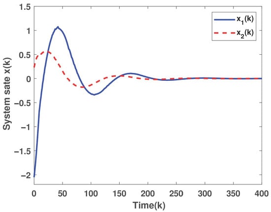
Figure 1. State trajectory of the closed-loop system.

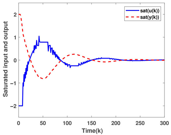
Figure 2. Saturated control input and measurement output.

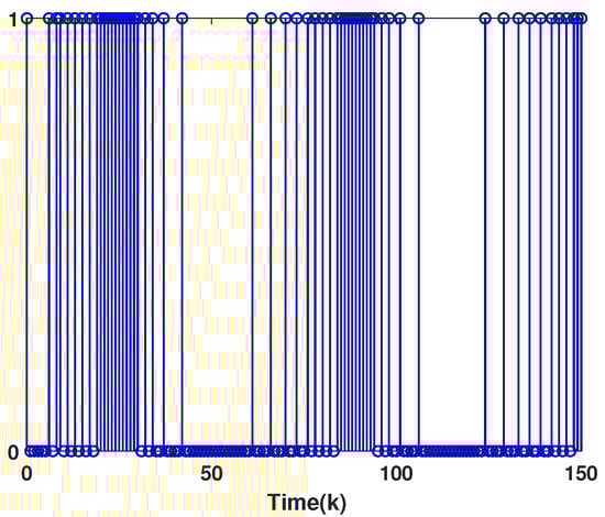
Figure 3. Triggering instants (1 → triggered, 0 → no triggered).

In Table 1, we list the event-triggering numbers and corresponding rates for different $\alpha$ over the time interval $[0,150]$. In the simulation, one sets $x_0={[-1.60.2]}^T\in \epsilon (X,1)$. As shown in the table, the number and the ETR are significantly reduced under the ETM-based design. Noting that the parameter $\alpha$ relates to the size of the admissible set of initial conditions, it can be observed that a larger admissible set generally leads to a higher ETR.

Table 1. Numbers and ETRs for different $\alpha$.

$\mathit{\alpha }$	0.8	0.9	1.0	1.05	1.1
Number	24	41	44	50	59
ETR (%)	15.89	27.15	29.14	33.11	39.07

Next, we address the scenario involving disturbances. By selecting parameters $\vartheta =10$, $\lambda =0.5$, $H_y={10}^{-4}$, and solving the optimization problem for $\delta$, we obtain ${\delta }_M=15.0657$. Then, choosing $\delta =10\le {\delta }_M$ solving the optimization problem for $\gamma$ yields ${\gamma }_m=4.6855$. However, directly implementing these $\delta$ and $\gamma$ values would render the ETM ineffective. To optimize the ETR, we set $\gamma =10$ (where $\gamma \ge {\gamma }_m$) and solve Prob. 2, obtaining

$$\begin{gathered} A_c=\left[\begin{array}{cc}0.8038& -0.1345\\ -0.0063& 0.0009\end{array}\right],B_c=\left[\begin{array}{c}-1.2129\\ 0.0090\end{array}\right],\hfill & \\ {C}_c=\left[\begin{array}{cc}0.0478& 0.0353\end{array}\right],E_c=\left[\begin{array}{c}4.1387\\ -0.8701\end{array}\right],\hfill & \\ {D}_c=-1.0004,{\Omega }_y=0.1231,{\Omega }_e=46.7965. \end{gathered}$$

Simulation using these parameters demonstrates that only 51 data packets are released over the interval $[0,100]$, confirming the ETM’s effectiveness in conserving network resources. In the simulation, $w\left(k\right)$ is set as $w\left(0\right)=w\left(1\right)=\sqrt{5}$ with $w\left(k\right)=0$ for $k\ge 2$.

Example 2.

The state-space representation of an inverted pendulum is given by [44]

$$\dot{x}\left(t\right)=\left[\begin{array}{cc}0& 1\\ {\displaystyle \frac{3(\mathbf{M}+\mathbf{m})\mathbf{g}}{\mathbf{l}(4\mathbf{M}+\mathbf{m})}}& 0\end{array}\right]x\left(t\right)+\left[\begin{array}{c}0\\ {\displaystyle \frac{3}{\mathbf{n}(4\mathbf{M}+\mathbf{m})}}\end{array}\right]u\left(t\right).\hfill$$

Let the parameters be $\mathbf{M}=8.0\mathrm{kg}$, $\mathbf{m}=2.0\mathrm{kg}$, $\mathbf{n}=0.8\mathrm{m}$, $\mathbf{g}=9.8\mathrm{m}/{\mathrm{s}}^2$, with a sampling time of $T_s=30\mathrm{ms}$. The discretized model of the system can then be expressed as [44]

$$x(k+1)=\left[\begin{array}{cc}1.0078& 0.0301\\ 0.5202& 1.0078\end{array}\right]x\left(k\right)+\left[\begin{array}{c}-0.0001\\ -0.0053\end{array}\right]u\left(k\right).\hfill$$

The system measurement output is $y\left(k\right)=\left[11\right]x\left(k\right)$. Furthermore, it is assumed that the system is subject to actuator and sensor saturations with ${\overline{u}}_1=50$ and ${\overline{y}}_1=1$.

Let $\vartheta =10$, $\lambda =0.5$, $H_y={10}^{-4}$, $\alpha =0.4$, $S=I$, and solve Prob. 1 to obtain

$$\begin{array}{l}{A}_c=\left[\begin{array}{cc}1.0263& 0.0129\\ -0.0107& -0.0002\end{array}\right],B_c=\left[\begin{array}{c}0.1470\\ -0.0015\end{array}\right],\hfill \\ C_c=\left[\begin{array}{cc}-66.2250& 1.2718\end{array}\right],D_c=-139.8100,\hfill \\ {\Omega }_y=0.3755,{\Omega }_e=12.5690,\hfill \\ E_c={10}^{-3}\left[\begin{array}{c}-0.8751\\ -0.3152\end{array}\right],X=\left[\begin{array}{cc}6.2175& 0.3498\\ 0.3498& 2.4841\end{array}\right].\hfill \end{array}$$

Using the above parameters with $x_0={\left[0.370.19\right]}^T\in \epsilon (X,1)$, we plot the closed-loop system’s state trajectory, saturated control input and measurement output, as well as data-triggering instants. Figure 4 confirms that closed-loop stabilization is successfully achieved. Figure 5 shows that the actuator experiences saturation during the initial period. Finally, Figure 6 demonstrates that the ETM effectively reduces the number of data transmissions.

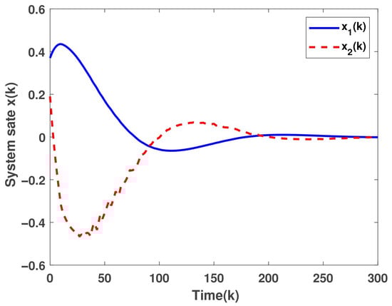
Figure 4. State trajectory of the closed-loop system.

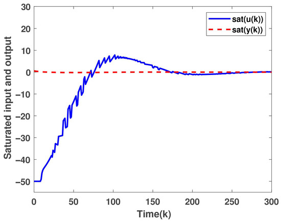
Figure 5. Saturated control input and measurement output.

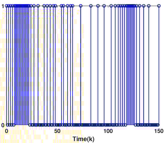
Figure 6. Triggering instants (1 → triggered, 0 → no triggered).

5. Conclusions

This paper has investigated the co-design of an event-triggered dynamic output feedback controller for discrete-time linear systems under dual saturation constraints. A dynamic ETM incorporating generalized weighting parameters is proposed, and sufficient LMI-based conditions are established using a Lyapunov approach combined with generalized sector conditions. Convex optimization problems are further formulated to maximize the ETR under guaranteed closed-loop performance. Numerical simulations demonstrate that the proposed scheme effectively reduces communication frequency while preserving desirable system performance. The developed framework offers a practical design tool for NCSs operating under bandwidth limitations and physical saturation constraints, with direct applications in self-balancing robotic platforms such as two-wheeled autonomous vehicles and legged robots. Future research focus on: (1) extending the approach to time-delay systems and multi-agent systems [18,26,32]; (2) incorporating actuator rate constraints alongside amplitude saturation [3]; and (3) developing adaptive and neural network-based strategies for nonlinear systems with unknown parameters [5,45].

References

- Chen, H.; Zhou, P.; Yang, R.; Chen, Y. Trajectory tracking control by PCH method for AUVs with input saturations. Int. J. Syst. Sci. 2025, 56, 3512–3527. [Google Scholar] [CrossRef]
- Ding, L.; Sun, W. Predefined time fuzzy adaptive control of switched fractional-order nonlinear systems with input saturation. Int. J. Netw. Dyn. Intell. 2023, 2, 100019. [Google Scholar] [CrossRef]
- Jin, X.; Qin, J.; Shi, Y.; Zheng, W.X. Auxiliary fault tolerant control with actuator amplitude saturation and limited rate. IEEE Trans. Syst. Man Cybern. Syst. 2017, 48, 1816–1825. [Google Scholar] [CrossRef]
- Liang, Y.; Xie, M.; Zhang, J.; Ming, Z.; Gao, Z. Integral reinforcement learning-based stochastic guaranteed cost control for time-varying systems with asymmetric saturation actuators. Actuators 2025, 14, 506. [Google Scholar] [CrossRef]
- Zhang, H.; Xiang, Z. Finite-time robust adaptive simultaneous stabilisation of nonlinear time-delay systems with actuator saturation. Int. J. Syst. Sci. 2024, 55, 49–67. [Google Scholar] [CrossRef]
- Tarbouriech, S.; Garcia, G.; Gomes da Silva, J.-M., Jr.; Queinnec, I. Stability and Stabilization of Linear Systems with Saturating Actuators; Springer: London, UK, 2011. [Google Scholar]
- Zhou, B.; Lin, Z.; Duan, G. A parametric Lyapunov equation approach to the design of low gain feedback. IEEE Trans. Autom. Control 2008, 53, 1548–1554. [Google Scholar] [CrossRef]
- Zhou, B. Analysis and design of discrete-time linear systems with nested actuator saturations. Syst. Control Lett. 2013, 62, 871–879. [Google Scholar] [CrossRef]
- Chen, Y.; Wang, Z. Local stabilization for discrete-time systems with distributed state delay and fast-varying input delay under actuator saturations. IEEE Trans. Autom. Control 2021, 66, 1337–1344. [Google Scholar] [CrossRef]
- Chen, Y.; Wang, Z.; Shen, B.; Han, Q.-L. Local stabilization for multiple input-delay systems subject to saturating actuators: The continuous-time case. IEEE Trans. Autom. Control 2022, 67, 3090–3097. [Google Scholar] [CrossRef]
- Bu, X.; Hou, Z.; Yu, Q.; Yang, Y. Quantized data driven iterative learning control for a class of nonlinear systems with sensor saturation. IEEE Trans. Syst. Man Cybern. Syst. 2020, 50, 5119–5129. [Google Scholar] [CrossRef]
- Turner, M.C.; Tarbouriech, S. Anti-windup compensation for systems with sensor saturation: A study of architecture and structure. Int. J. Control 2009, 82, 1253–1266. [Google Scholar] [CrossRef]
- Yang, F.; Li, Y. Set-membership filtering for systems with sensor saturation. Automatica 2009, 45, 1896–1902. [Google Scholar] [CrossRef]
- Garcia, G.; Tarbouriech, S.; Gomes da Silva, J.M., Jr.; Eckhard, D. Finite L2 gain and internal stabilisation of linear systems subject to actuator and sensor saturations. IET Control Theory Appl. 2009, 3, 799–812. [Google Scholar] [CrossRef]
- Wang, Z.; Ho, D.W.C.; Dong, H.; Gao, H. Robust H∞ finite-horizon control for a Class of stochastic nonlinear time-varying systems subject to sensor and actuator saturations. IEEE Trans. Autom. Control. 2010, 55, 1716–1722. [Google Scholar] [CrossRef]
- Hespanha, J.P.; Naghshtabrizi, P.; Xu, Y. A survey of recent results in networked control systems. Proc. IEEE 2007, 95, 138–162. [Google Scholar] [CrossRef]
- Lu, Z.; Guo, G. Control and communication scheduling co-design for networked control systems: A survey. Int. J. Syst. Sci. 2023, 54, 189–203. [Google Scholar] [CrossRef]
- Talebi, S.P.; Werner, S.; Huang, Y.-F.; Gupta, V. Distributed algebraic Riccati equations in multi-agent systems. In Proceedings of the 2022 European Control Conference, London, UK, 12–15 July 2022; pp. 1810–1817. [Google Scholar]
- Chen, Y.; Zhang, K.; Zhao, Y. Synchronization control for delayed neural networks under Round-Robin protocol and input saturations. Neurocomputing 2025, 645, 130474. [Google Scholar] [CrossRef]
- Ding, D.; Wang, Z.; Han, Q.-L.; Wei, G. Neural-network-based output-feedback control under Round-Robin scheduling protocols. IEEE Trans. Cybern. 2019, 49, 2372–2384. [Google Scholar] [CrossRef]
- Jin, F.; Ma, L.; Zhao, C.; Liu, Q. State estimation in networked control systems with a real-time transport protocol. Syst. Sci. Control Eng. 2024, 12, 2347885. [Google Scholar] [CrossRef]
- Li, C.; Liu, Y.; Gao, M.; Sheng, L. Fault-tolerant formation consensus control for time-varying multi-agent systems with stochastic communication protocol. Int. J. Netw. Dyn. Intell. 2024, 3, 100004. [Google Scholar] [CrossRef]
- Wang, W.; Ma, L.; Rui, Q.; Gao, C. A survey on privacy-preserving control and filtering of networked control systems. Int. J. Syst. Sci. 2024, 55, 2269–2288. [Google Scholar] [CrossRef]
- Girard, A. Dynamic triggering mechanisms for event-triggered control. IEEE Trans. Autom. Control 2015, 60, 1992–1997. [Google Scholar] [CrossRef]
- Peng, C.; Li, F. A survey on recent advances in event-triggered communication and control. Inform. Sci. 2018, 457, 113–125. [Google Scholar] [CrossRef]
- Ge, C.; Ma, L.; Xu, S. Distributed fixed-time leader-following consensus for multi-agent systems: An event-triggered mechanism. Actuators 2024, 13, 40. [Google Scholar] [CrossRef]
- Yue, D.; Tian, E.; Han, Q.-L. A delay system method for designing event-triggered controllers of networked control systems. IEEE Trans. Autom. Control 2013, 58, 475–481. [Google Scholar] [CrossRef]
- Dai, D.; Li, J.; Song, Y.; Yang, F. Event-based recursive filtering for nonlinear bias-corrupted systems with amplify-and-forward relays. Syst. Sci. Control Eng. 2024, 12, 2332419. [Google Scholar] [CrossRef]
- Liu, X.; Zeng, P.; Deng, F.; Wu, Z.-H.; Li, M. Event-triggered L2-L∞ control for discrete-time Markov jump systems with DoS attacks and exogenous disturbance. Int. J. Syst. Sci. 2024, 55, 16–32. [Google Scholar] [CrossRef]
- Qian, W.; Wu, Y.; Shen, B. Novel adaptive memory event-triggered-based fuzzy robust control for nonlinear networked systems via the differential evolution algorithm. IEEE/CAA J. Autom. Sin. 2024, 11, 1836–1848. [Google Scholar] [CrossRef]
- Yang, J.; Chen, Y.; Ma, L.; Yang, J. Event-triggered regional stabilization for T-S fuzzy systems subject to communication delays and actuator saturations. J. Franklin. Inst. 2024, 361, 106653. [Google Scholar] [CrossRef]
- Zhang, R.; Liu, H.; Liu, Y.; Tan, H. Dynamic event-triggered state estimation for discrete-time delayed switched neural networks with constrained bit rate. Syst. Sci. Control Eng. 2024, 12, 2334304. [Google Scholar] [CrossRef]
- Chen, Y.; Zhao, Y.; Gu, Z.; Yang, X. Anti-windup design for networked time-delay systems subject to saturating actuators under round-robin protocol. Appl. Math. Comput. 2025, 499, 129413. [Google Scholar] [CrossRef]
- Huang, K.; Pan, F. Fault detection for nonlinear networked control systems with sensor saturation and random faults. IEEE Access 2020, 8, 92541–92551. [Google Scholar] [CrossRef]
- Yang, H.; Xia, Y.; Yuan, H.; Yan, J. Quantized stabilization of networked control systems with actuator saturation. Int. J. Robust Nonlinear Control 2016, 26, 3595–3610. [Google Scholar] [CrossRef]
- Chen, Y.; Liu, H.; Hu, J.; Lin, H. Dynamic event-triggered regional synchronization for discrete-time delayed dynamical networks: Dealing with saturating actuators. Neurocomputing 2025, 653, 131179. [Google Scholar] [CrossRef]
- Liu, D.; Yang, G.-H. Event-triggered non-fragile control for linear systems with actuator saturation and disturbances. Inform. Sci. 2018, 429, 1–11. [Google Scholar] [CrossRef]
- Luo, L.; Chen, Y.; Jia, J.; Zhao, K.; Jia, J. Event-triggered anti-windup strategy for time-delay systems subject to saturating actuators. AIMS Math. 2024, 9, 27721–27738. [Google Scholar] [CrossRef]
- Ma, L.; Wang, Z.; Cai, C.; Alsaadi, F.E. A dynamic event-triggered approach to H∞ control for discrete-time singularly perturbed systems with time-delays and sensor saturations. IEEE Trans. Syst. Man Cybern. Syst. 2020, 51, 6614–6625. [Google Scholar] [CrossRef]
- Moreira, L.G.; Groff, L.B.; Gomes da Silva, J.M., Jr. Event-triggered state-feedback control for continuous-time plants subject to input saturation. J. Control Autom. Elec. Syst. 2016, 27, 473–484. [Google Scholar] [CrossRef]
- Souza, C.D.; Tarbouriech, S.; Leite, V.J.S.; Castelan, E.B. Co-design of an event-triggered dynamic output feedback controller for discrete-time LPV systems with constraints. J. Franklin. Inst. 2022, 359, 697–718. [Google Scholar] [CrossRef]
- Zuo, Z.; Guan, S.; Wang, Y.; Li, H. Dynamic event-triggered and self-triggered control for saturated systems with anti-windup compensation. J. Franklin. Inst. 2017, 354, 7624–7642. [Google Scholar] [CrossRef]
- Li, L.; Zou, W.; Fei, S. Event-based dynamic output-feedback controller design for networked control systems with sensor and actuator saturations. J. Franklin. Inst. 2017, 354, 4331–4352. [Google Scholar] [CrossRef]
- Zhang, J.; Peng, C.; Zheng, M. Improved results for linear discrete-time systems with an interval time-varying input delay. Int. J. Syst. Sci. 2016, 47, 492–499. [Google Scholar] [CrossRef]
- Jin, X.; Lu¨, S.; Yu, J. Adaptive NN-based consensus for a class of nonlinear multi-agent systems with actuator faults and faulty networks. IEEE Trans. Neural Netw. Learn. Syst. 2021, 33, 3474–3486. [Google Scholar] [CrossRef] [PubMed]
Disclaimer/Publisher’s Note: The statements, opinions and data contained in all publications are solely those of the individual author(s) and contributor(s) and not of MDPI and/or the editor(s). MDPI and/or the editor(s) disclaim responsibility for any injury to people or property resulting from any ideas, methods, instructions or products referred to in the content. |
© 2025 by the authors. Licensee MDPI, Basel, Switzerland. This article is an open access article distributed under the terms and conditions of the Creative Commons Attribution (CC BY) license (https://creativecommons.org/licenses/by/4.0/).