Dynamic Mechanistic–Data-Driven Hybrid Modeling of the Main Distributing Valve in a Hydroturbine Governor

Abstract

The main distributing valve (MDV) plays a core role in hydraulic amplification and precise control within the hydro-turbine governing system, and its spool position dynamics directly affect the regulation quality and stability of the hydro-turbine generator unit. However, developing a high-fidelity dynamic model of the MDV remains challenging, as existing methods typically rely on linearization assumptions and fail to fully account for system uncertainties, resulting in limited accuracy and poor cross-condition stability. To address this issue, this paper proposes a mechanistic–data-driven hybrid modeling method. Firstly, a modular modeling strategy is adopted to accurately construct a nonlinear mechanism-based model (MBM) that conforms to the actual industrial system. Secondly, to address the unknown dynamics not captured by the MBM, a Bayesian optimization-enhanced Light Gradient Boosting Machine (BO-LightGBM) model is developed. Then, a cascade–additive architecture is employed to achieve effective integration of the two. Finally, verification experiments are conducted under various dynamic processes based on the actual operating data of the governor. The results show that the proposed hybrid model significantly outperforms the other five comparison models in terms of accuracy and stability while retaining physical interpretability. This provides a more practically valuable solution for the dynamic modeling and simulation of hydroturbine actuators.

1. Introduction

As the penetration rate of renewable energy in power systems continues to rise, the volatility and uncertainty of power grids have increased significantly, placing higher demands on the operational stability and dynamic regulation capability of power systems [1,2]. Hydropower, with its excellent regulation performance, plays an irreplaceable role in mitigating the output fluctuations of renewable energy, maintaining power grid frequency stability, and ensuring the balance between power supply and demand [3,4,5,6]. The hydro-turbine governing system (HTGS) is the core control unit of hydroelectric generating units, typically consisting of a microcomputer regulator, an electro-hydraulic servo system, and a controlled object [7,8]. As a hydraulic amplifier in the servo system [9], the dynamic performance of the main distributing valve (MDV)—including displacement response speed, accuracy, and stability—exerts a decisive impact on the control quality of the HTGS [10,11]. Therefore, constructing a high-precision dynamic model of the MDV position is a crucial link in identifying potential instability risks of HTGS, optimizing the system’s regulation quality, and ensuring power grid frequency stability.

Currently, most studies incorporate the MDV into the modeling framework as a component module of the HTGS [12,13]. The HTGS is a complex and nonlinear system [14,15]; researchers often focus on its overall modeling while ignoring or simplifying the nonlinear characteristics and dynamic response process of the MDV. This may affect the accuracy of the overall model in describing the dynamic behavior of the actual system under high-precision regulation or complex operating conditions. For instance, Lu et al. [16] considered the delay link and amplitude limiting link, established a nonlinear governing system model with different control modes, but neglected the nonlinear characteristics of the MDV. To reduce the overall complexity of the model and facilitate subsequent analysis, previous studies [8,17] simplified the MDV model into a linear model and established the transfer function model of the governor. Some scholars also conduct modeling research on the MDV or hydraulic servo system as independent objects, aiming to reveal their internal working mechanisms and dynamic characteristics more accurately. For example, Zhou et al. [18] established a linear model of the governor’s MDV device based on the structure and working principle; Wu et al. [19] established a mechanistic model of the MDV using hydraulic simulation software and studied its response speed characteristics; Xia et al. [20] built a simulation model of the electro-hydraulic servo system based on the hydraulic simulation modules provided by SimHydraulics software; Yan et al. [21] added a speed limiting link to the linear model of the servo system to establish a nonlinear model; Milic et al. [22] used Linear Fractional Transformation (LFT) to describe the uncertainty of model parameters in the servo system.

However, despite these efforts, most existing models still rely on linear simplifications, which limit their ability to accurately represent the system’s complex dynamic behavior. Stosiak et al. [23] further demonstrated that the dynamic response of a directional control valve exhibits pronounced nonlinearities—especially when the spool is overdriven or subjected to external vibrations—resulting in pressure pulsations and oscillatory behaviors that cannot be represented by linear models. These findings highlight the necessity of incorporating nonlinear dynamic characteristics when modeling valve systems.

In practical engineering applications, the accuracy of the models is often affected by various factors [24]. For example, time-varying parameters, individual differences in valves, and changes in component performance over time [25] will all increase model errors, thereby affecting the accuracy and reliability of simulation results.

Benefiting from the rapid development of machine learning algorithms, mechanistic–data-driven hybrid modeling methods have received increasing attention in the modeling of complex industrial systems and demonstrated significant advantages [26,27,28,29,30]. For example, aiming at the problems of poor modeling accuracy and significant uncertainty of traditional mechanistic models, Zhang et al. [31] propose a hybrid modeling method combining neural networks and mechanistic models, which not only achieves high-precision modeling but also overcomes the defect of weak adaptability of single models. Another example is given in [32], which realizes the complementary advantages of the mechanism-based approach and the data-driven approach by fusing them, enhancing the accuracy and physical interpretability of the model.

In view of this, to characterize the dynamic behavior of the governor’s MDV and accurately simulate the position response process of the valve spool, this paper proposes a mechanistic–data-driven hybrid modeling method. The main work is as follows:

(1)

Based on the structural characteristics and working mechanism of the MDV, a modular modeling strategy is adopted to construct a mechanism-based model (MBM) framework covering electromechanical-hydraulic multi-domain coupling. By accurately mapping the physical interaction relationships of each module, the physical interpretability of the model is fundamentally ensured.

(2)

A Bayesian optimization-enhanced Light Gradient Boosting Machine (BO-LightGBM) model is developed, aiming to efficiently learn the complex dynamic characteristics and system uncertainties that cannot be explained by the MBM.

(3)

The MBM serves as the physical backbone of the entire system, reducing the BO-LightGBM model’s dependence on learning full-scale physical features. The effective integration of mechanism knowledge and data information is achieved through a cascade–additive approach, making up for the deficiency of the MBM in describing complex nonlinear factors.

(4)

Based on the actual operating dataset of the governor, comparative experiments are conducted under 4 typical dynamic processes—start-up, load increasing, shutdown, and load rejection—to verify the simulation accuracy and adaptability of the proposed modeling method in practical engineering scenarios.

2. Modular Modeling Method Based on the Mechanism of the MDV

2.1. Structure and Control Principle of the Servo System

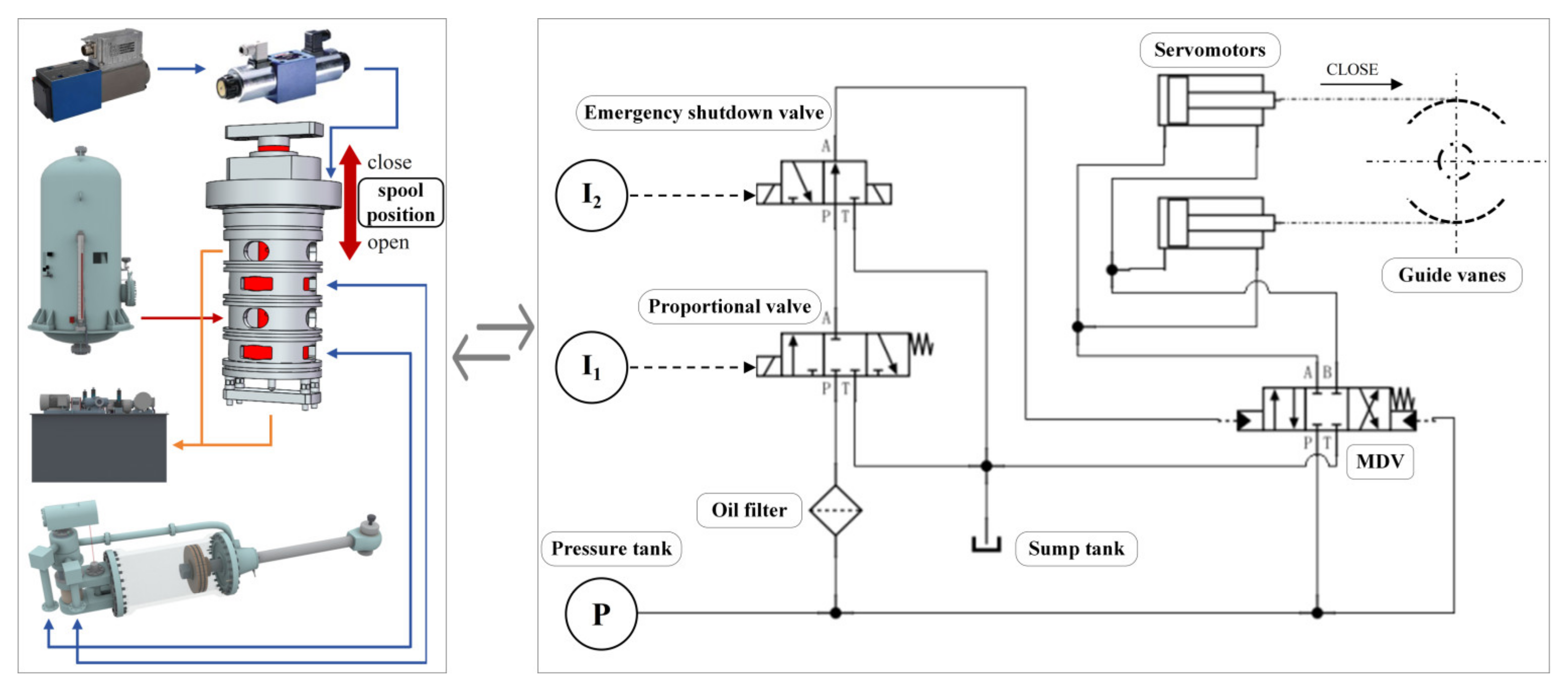
The MDV device is a core component of the governor’s servo system, typically composed of components such as the MDV, electro-hydraulic converter, emergency shutdown valve (ESV), and oil filter [33]. The MDV, also known as a control valve, is a distributing valve that controls the actuation of the servomotor (a hydraulic actuator that drives the hydro-turbine guide vanes via linear displacement).

The structure of the servo system, which employs a proportional valve as the main electro-hydraulic converter, is shown in Figure 1. In the system, the main pressure oil from the oil pressure supply unit is divided into two paths upon entering the MDV: one path directly enters the main pressure chamber and constant-pressure chamber of the MDV, while the other passes sequentially through the proportional valve and ESV before entering the control chamber of the MDV. The pressure difference between the control chamber and the constant-pressure chamber generates a net force on the MDV spool (piston), driving its displacement and enabling precise control of the spool position. As the MDV spool moves, the opening areas and on-off states of the valve ports change, directing the high-pressure oil into either the rodless or the rod chamber of the servomotor [34,35]. The hydraulic pressure difference drives the servomotor in linear motion, which, through linkages and levers, actuates the hydro-turbine guide vane position. Meanwhile, the servomotor position serves as a feedback signal to the system and, together with the opening command, controls the position of the MDV spool.

Figure 1. Structure of the governor servo system.

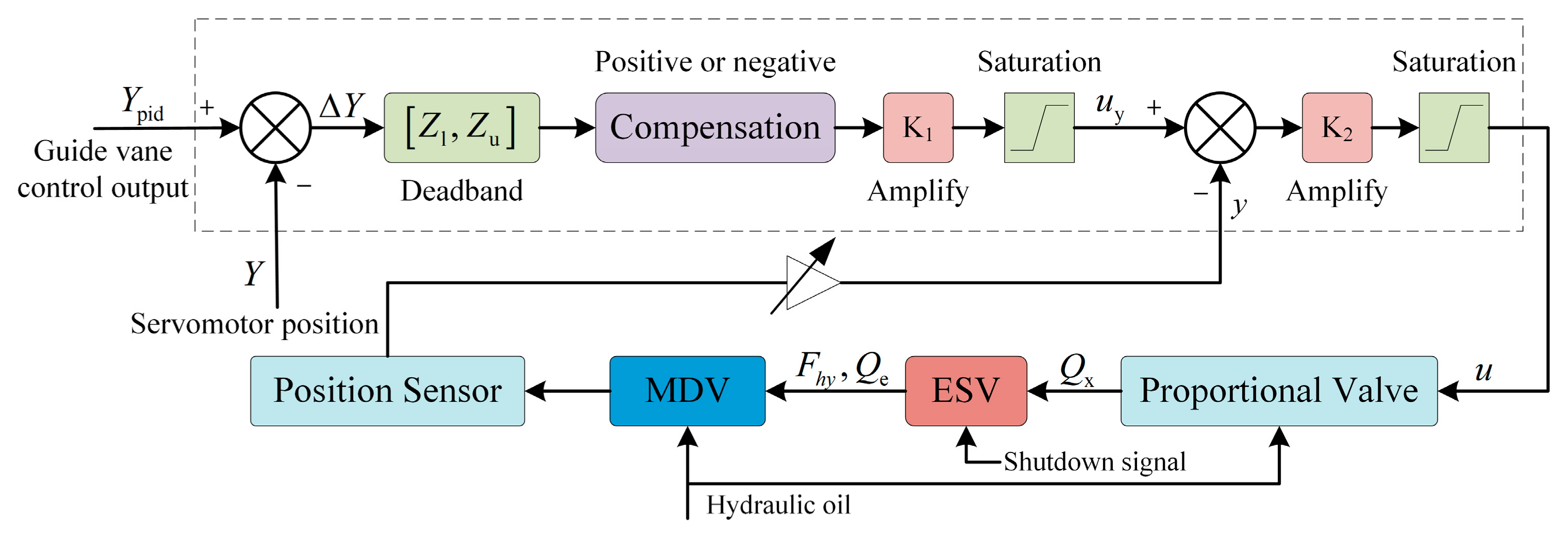
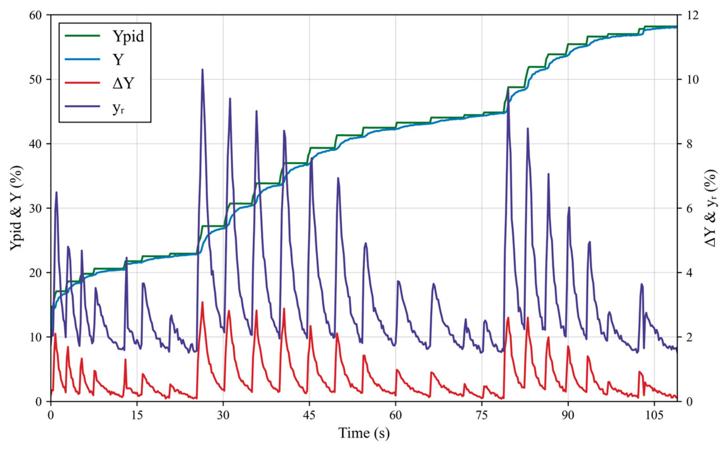
As shown in Figure 2, after comparing the opening command signal $Y_{\mathrm{p}\mathrm{i}\mathrm{d}}$ with the position feedback signal $Y$ of the servomotor, the microcomputer regulator obtains the difference $∆Y$ between them, which forms the basic input signal for the system’s closed-loop control. The dynamic response of the MDV to these control input variations during the load-increasing process is illustrated in Figure 3, showing how the valve spool reacts to changes in the control signal in real time. The signal then undergoes processes such as deadband, compensation, amplification, and amplitude limiting to generate the position control signal for the MDV:

$$u_{\mathrm{c}}(t)=\left\{\begin{array}{ll}{K}_1(Y_{\mathrm{pid}}(t)-Y(t))+C_{\mathrm{p}},\hfill & Y_{\mathrm{pid}}(t)-Y(t)\ge Z_{\mathrm{u}}\hfill \\ K_1(Y_{\mathrm{pid}}(t)-Y(t))+C_{\mathrm{n}},\hfill & Y_{\mathrm{pid}}(t)-Y(t)\le Z_{\mathrm{l}}\hfill \\ 0,\hfill & Z_{\mathrm{l}}<Y_{\mathrm{pid}}(t)-Y(t)<Z_{\mathrm{u}}\hfill \end{array}\right.$$

(1)

$$u_{\mathrm{y}}(t)=\mathrm{sat}(u_{\mathrm{c}}(t))$$

(2)

where $K_1$ is the large-loop gain coefficient, $C_{\mathrm{p}}$ is the positive compensation coefficient, $C_1$ is the negative compensation coefficient, $Z_{\mathrm{u}}$ is the upper limit of the deadband, $Z_{\mathrm{l}}$ is the lower limit of the deadband, and $\mathrm{s}\mathrm{a}\mathrm{t}\left(x\right)$ is the saturation function.

Figure 2. Automatic regulation principle of the MDV.

Figure 3. Dynamic response of the MDV to control input variations.

The saturation function limits the input within a specified range and is defined as:

$$\mathrm{sat}(x)=\left\{\begin{array}{ll}{x}_{\min },\hfill & x\le x_{\min }\hfill \\ x,\hfill & x_{\min }<x<x_{\max }\hfill \\ x_{\max },\hfill & x\ge x_{\min }\hfill \end{array}\right.$$

(3)

Next, the summation and amplification module compares $u_{\mathrm{y}}\left(t\right)$ with the MDV position feedback signal $y\left(t\right)$, amplifies the difference, and generates the control signal for driving the proportional valve:

$$u(t)=\mathrm{sat}(K_2(u_{\mathrm{y}}(t)-{\displaystyle \frac{y(t)}{y_{\mathrm{r}}}})+I_{\mathrm{r}})$$

(4)

where $K_2$ is the small-loop gain coefficient, $I_r$ is the current reference value of the proportional valve, and $y_r$ is the position reference value of the MDV.

Finally, the proportional valve converts the input electrical control signal $u\left(t\right)$ into a hydraulic signal, which acts on the control end of the MDV, thereby establishing a pressure difference between the control chamber and the constant-pressure chamber.

2.2. Mechanism Modeling of the Proportional Valve

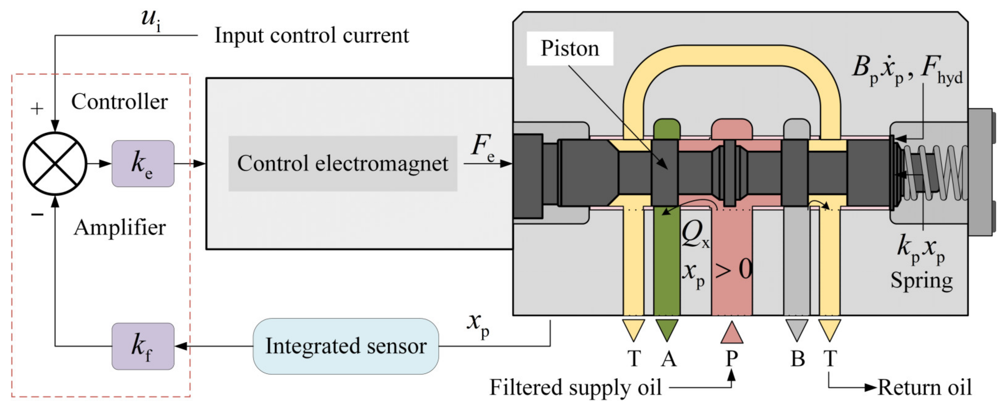
To establish the mathematical model of the proportional valve, its internal structure and working principle are illustrated in Figure 4. The valve is primarily composed of a valve body, piston, electromagnet, and an internal displacement sensor. By applying a continuously varying electrical signal (current or voltage) to the electromagnet, the valve can precisely and proportionally control its output flow. Meanwhile, the piston displacement is measured in real time by an integrated sensor and fed back to the amplifier, forming a closed-loop system for accurate valve positioning.

Figure 4. Schematic diagram of the proportional valve with an integrated amplifier and internal displacement sensor.

During operation, the piston is driven by the electromagnetic force generated by the electromagnetic coil within the electromagnet and is simultaneously subjected to other forces, including the spring force, viscous damping, and hydraulic forces. Among the hydraulic forces, the steady-state flow-induced component is considered in this work, while the transient hydrodynamic forces arising from rapid momentum changes in the fluid jet are neglected, as their magnitude is comparatively small under typical operating conditions [36,37]. Accordingly, the force balance equation of the proportional valve piston can be expressed as:

$$F_{\mathrm{e}}=m_{\mathrm{p}}{\ddot{x}}_{\mathrm{p}}+B_{\mathrm{p}}{\dot{x}}_{\mathrm{p}}+k_{\mathrm{p}}{x}_{\mathrm{p}}+F_{\mathrm{hyd}}$$

(5)

where $F_{\mathrm{e}}$ denotes the output force of the electromagnetic coil, $x_{\mathrm{p}}$ is the displacement of the proportional valve piston, $m_{\mathrm{p}}$ is the mass of the proportional valve piston, $k_{\mathrm{p}}$ is the stiffness of the spring, $B_{\mathrm{p}}$ is the viscous damping coefficient, and $F_{\mathrm{h}\mathrm{y}\mathrm{d}}$ is the steady-state hydraulic force.

$$F_{\mathrm{e}}=k_{\mathrm{e}}(u_{\mathrm{i}}-k_{\mathrm{f}}{x}_{\mathrm{p}})$$

(6)

$$F_{\mathrm{hyd}}=2C_{\mathrm{d}}{C}_{\mathrm{\nu }}{w}_{\mathrm{p}}\Delta p\cos \theta x_{\mathrm{p}}$$

(7)

where $k_{\mathrm{e}}$ is the electromagnet gain, $u_{\mathrm{i}}$ is the input current, $k_{\mathrm{f}}$ is the feedback coefficient of the position sensor, $C_{\mathrm{d}}$ is the flow coefficient, $C_{\mathrm{v}}$ is the flow velocity coefficient, ${\omega }_{\mathrm{p}}$ is the valve port area gradient, $∆p$ is the pressure difference across the valve port, and $\theta$ is the jet angle.

The steady-state hydraulic flow force model shown in Equation (7) follows the widely used formulation in proportional valve research [38]. When the pressure change is small, $2C_{\mathrm{d}}{C}_{\mathrm{\nu }}{w}_{\mathrm{p}}\Delta p\cos \theta$ can be approximately regarded as a constant, which we define as the hydraulic force stiffness coefficient $K_{\mathrm{h}}$. Therefore, we can obtain

$$F_{\mathrm{hyd}}\approx K_{\mathrm{h}}{x}_{\mathrm{p}}$$

(8)

Here, we define the equivalent stiffness as

$$K_{\mathrm{eq}}=k_{\mathrm{p}}+K_{\mathrm{h}}+k_{\mathrm{e}}{k}_{\mathrm{f}}$$

(9)

Thus, Equation (5) is simplified to

$$k_{\mathrm{e}}{u}_{\mathrm{i}}=m_{\mathrm{p}}{\ddot{x}}_{\mathrm{p}}+B_{\mathrm{p}}{\dot{x}}_{\mathrm{p}}+K_{\mathrm{eq}}{x}_{\mathrm{p}}$$

(10)

Performing Laplace transform on this second-order differential equation, the piston displacement-current transfer function can be obtained:

$$G(s)={\displaystyle \frac{K{\omega }_{\mathrm{n}}^2}{s^2+2\xi {\omega }_{\mathrm{n}}s+{\omega }_{\mathrm{n}}^2}}$$

(11)

where $K={\displaystyle \frac{k_e}{K_{eq}}}$, $\zeta ={\displaystyle \frac{B_p}{2\sqrt{m_p{K}_{eq}}}}$, and ${\omega }_n=\sqrt{{\displaystyle \frac{K_{eq}}{m_p}}}$.

The hydraulic part of the proportional valve adopts a spool valve structure. In this study, a zero neutral overlap condition is assumed, meaning that the spool lands align exactly with the orifice edges at the neutral position, so the valve ports are fully closed without positive or negative overlap. Under this assumption, the relative motion of the spool with respect to the valve sleeve forms a rectangular throttling orifice, through which the flow rate and direction of the hydraulic oil are regulated and can be expressed as

$$Q_{\mathrm{v}}=\left\{\begin{array}{cc}{C}_{\mathrm{d}}{\omega }_{\mathrm{p}}{x}_{\mathrm{p}}\sqrt{2\left(P_{\mathrm{p}}-P_{\mathrm{a}}\right)/\rho },& x_{\mathrm{p}}\ge 0\\ C_{\mathrm{d}}{\omega }_{\mathrm{p}}{x}_{\mathrm{p}}\sqrt{2\left(P_{\mathrm{a}}-P_{\mathrm{t}}\right)/\rho },& x_{\mathrm{p}}<0\end{array}\right.$$

(12)

where $P_{\mathrm{p}}$ is the oil pressure of the pressure tank, $P_{\mathrm{t}}$ is the return oil pressure, $P_a$ is the pressure at port A of the proportional valve, $P_b$ is the pressure at port B of the proportional valve, and $\rho$ is the density of the hydraulic oil.

When the pressure difference is 35 bar, the rated flow rate of the proportional valve is $Q_{\mathrm{n}}$, and the flow rate under other pressure differences can be considered as

$$Q_{\mathrm{x}}=\left\{\begin{array}{cc}{Q}_{\mathrm{n}}{x}_{\mathrm{p}}\sqrt{{\displaystyle \frac{P_{\mathrm{p}}-P_{\mathrm{a}}}{3.5}}},& x_{\mathrm{p}}\ge 0\\ Q_{\mathrm{n}}{x}_{\mathrm{p}}\sqrt{{\displaystyle \frac{P_{\mathrm{a}}-P_{\mathrm{t}}}{3.5}}},& x_{\mathrm{p}}<0\end{array}\right.$$

(13)

2.3. Mechanism Modeling of the Emergency Shutdown Valve

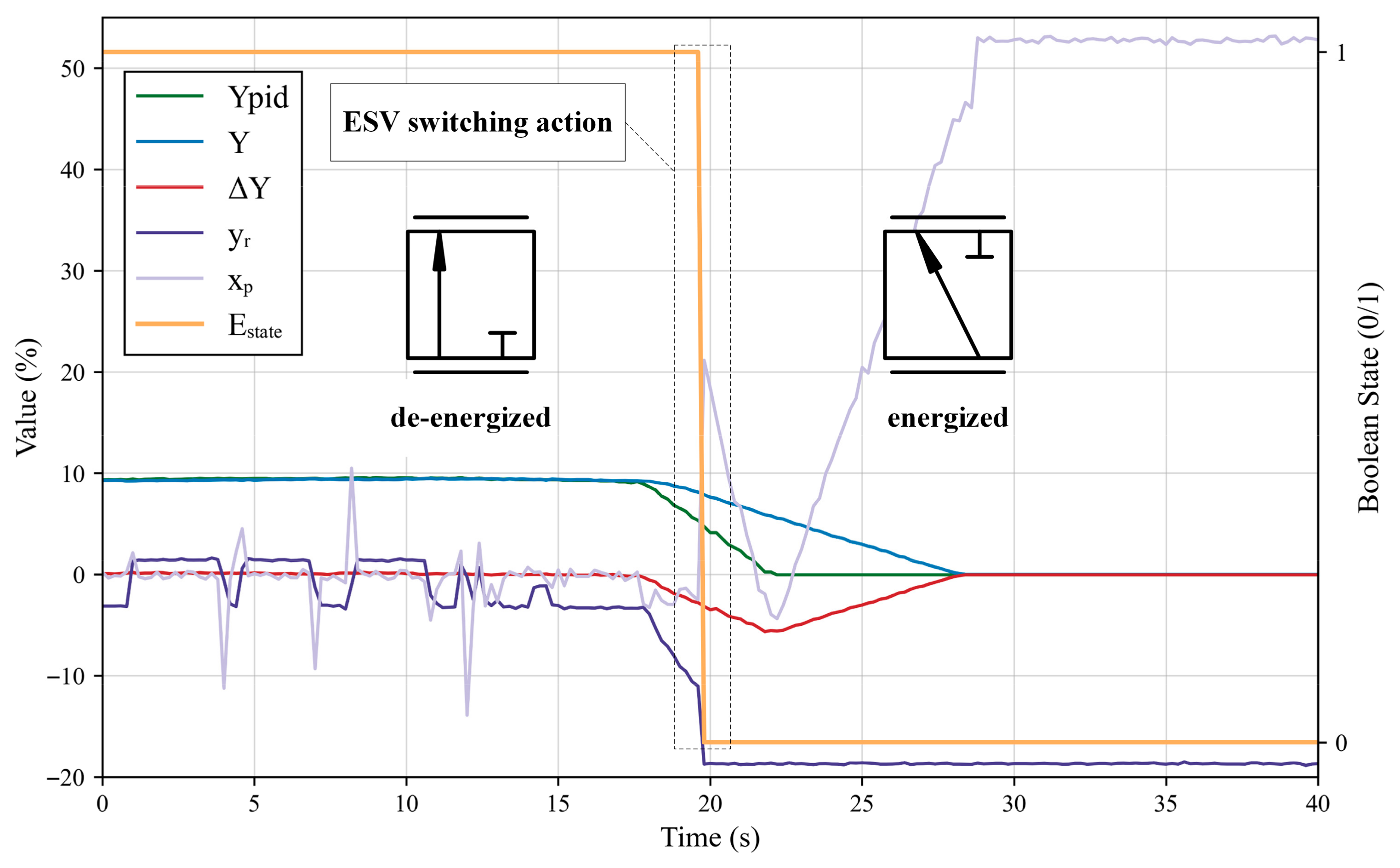
The Emergency Shutdown Valve (ESV) is positioned between the proportional valve (PV) and the MDV, serving as a critical component in the safety command execution chain. Under normal operating conditions, the ESV remains in its de-energized (rest) state, allowing the control oil from the proportional valve to act on the control chamber of the MDV, thereby maintaining the guide vane position as commanded by the governor. When the emergency shutdown solenoid valve receives a shutdown signal, its piston switches position immediately: the control oil from the proportional valve is cut off, and at the same time, the control chamber of the MDV is connected to the return oil, leading to the rapid closure of the guide vanes, as shown in Figure 5.

Figure 5. Time-domain responses of control signals and MDV position during the shutdown process.

The ESV is a 2-position 3-way solenoid directional valve, whose main function is to switch fluid paths. Ignoring the dynamic characteristics of the solenoid valve, the flow rate through the ESV can be described by the following function:

$$Q_{\mathrm{e}}=\left\{\begin{array}{ll}{C}_{\mathrm{d}}{A}_{\mathrm{e}}\sqrt{2(P_{\mathrm{e}}-P_{\mathrm{t}})/\rho },\hfill & E_{\mathrm{state}}=0\hfill \\ Q_{\mathrm{x}},\hfill & E_{\mathrm{state}}=1\hfill \end{array}\right.$$

(14)

where $A_e$ is the flow area of the ESV port, and $P_{\mathrm{e}}$ is the inlet pressure of the ESV.

2.4. Mechanism Modeling of the MDV

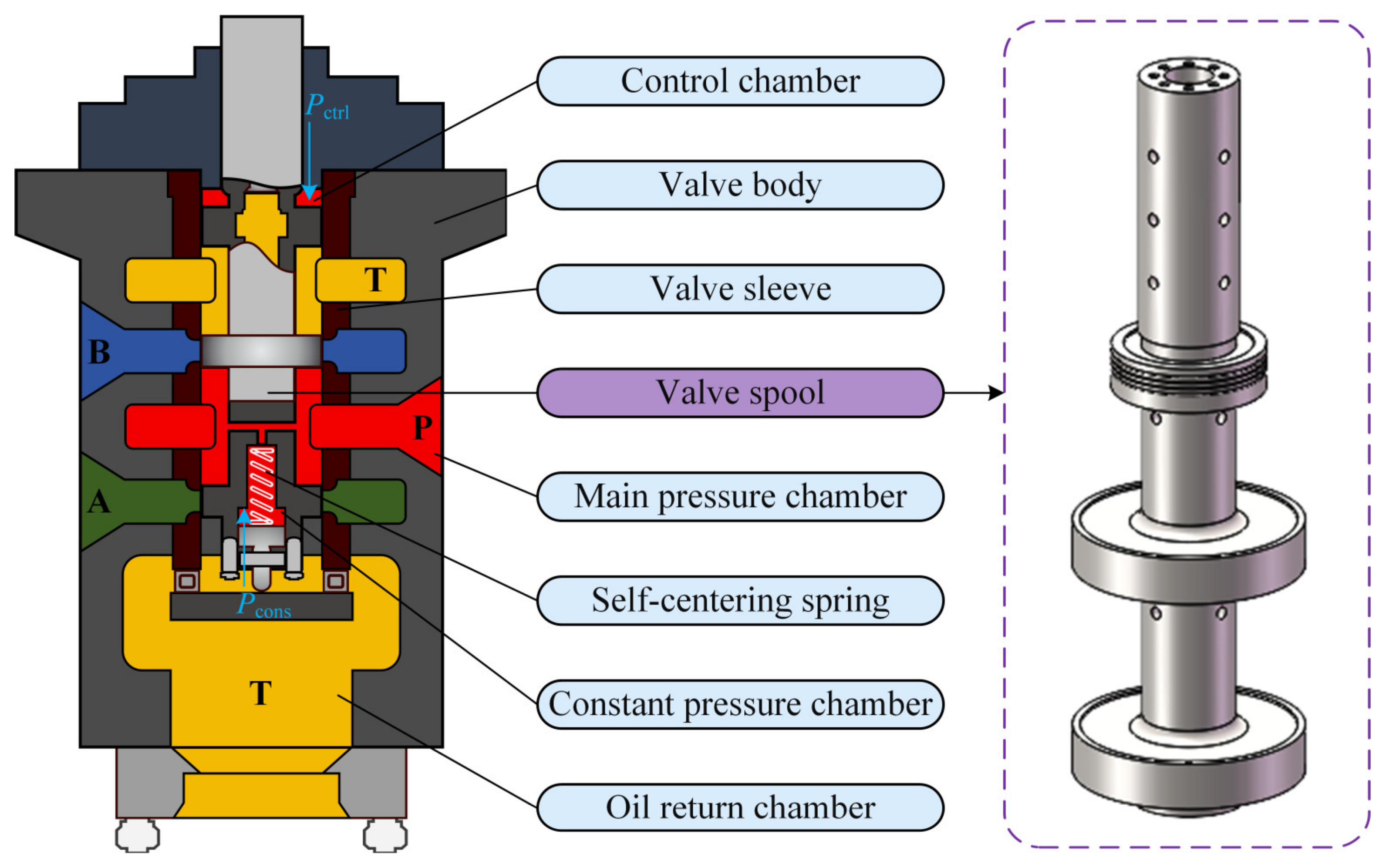
The MDV can be considered analogous to an oversized 3-position, 4-way directional valve with O-type function. Its primary components include the valve body, valve spool, valve sleeve, and a self-centering mechanism. As illustrated in Figure 6, the valve body houses the spool and sleeve, while the self-centering mechanism ensures that the spool returns to the neutral position when no pilot pressure is applied. In the neutral state, the spool lands slightly overlap the orifice edges, fully blocking all flow paths and ensuring a leakage-free closed state. When pilot pressure is applied to either side of the spool, the corresponding throttling area opens, directing high-pressure oil to the appropriate servomotor chamber while allowing return flow from the opposite chamber. Figure 6 also highlights the relative positions of the pilot pressure ports and internal flow passages, providing a clear view of the overall composition and functional layout of the MDV.

Figure 6. Composition and structure of the MDV.

Building on the structural and functional description of the MDV, the spool is subjected to multiple forces during operation, including inertia, viscous damping, hydraulic force, spring force, and gravity. These forces collectively determine the dynamic behavior of the spool, which can be captured using Newton’s second law. Accordingly, the motion of the spool can be described by the following differential equation:

$$F_{\mathrm{hy}}=m{\ddot{x}}_{\mathrm{m}}+B{\dot{x}}_{\mathrm{m}}+F_{\mathrm{k}}-mg$$

(15)

where $x_{\mathrm{m}}$ is the displacement of the MDV spool, $m$ is the mass of the spool, $g$ is the gravitational acceleration, $B$ is the viscous damping coefficient, $F_{\mathrm{k}}$ is the spring force, and $F_{\mathrm{h}\mathrm{y}}$ represents the hydraulic force acting on the spool.

The hydraulic force is generated by the pressure difference between the control chamber and the constant-pressure chamber, and can be expressed as

$$F_{\mathrm{hy}}=P_{\mathrm{ctrl}}{A}_{\mathrm{ctrl}}-P_{\mathrm{cons}}{A}_{\mathrm{cons}}$$

(16)

where $A_{\mathrm{c}\mathrm{t}\mathrm{r}\mathrm{l}}$ is the effective acting area of the control chamber, $A_{\mathrm{c}\mathrm{o}\mathrm{n}\mathrm{s}}$ is the effective acting area of the constant-pressure chamber, $P_{\mathrm{c}\mathrm{t}\mathrm{r}\mathrm{l}}$ is the pressure of the control chamber, and $P_{\mathrm{c}\mathrm{o}\mathrm{n}\mathrm{s}}$ is the pressure of the constant-pressure chamber.

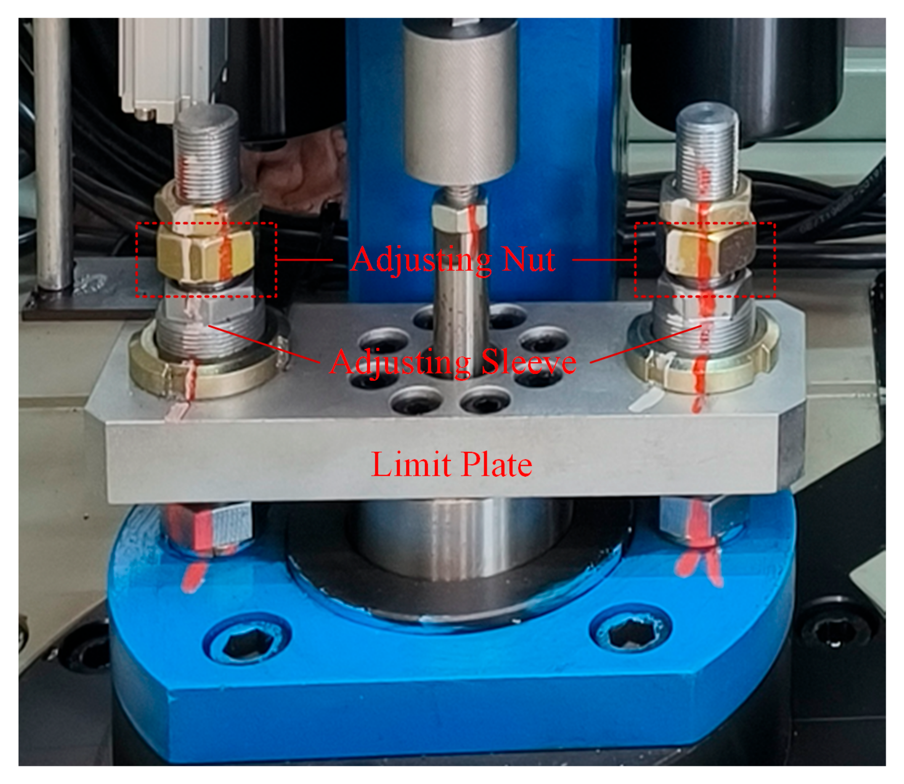
As shown in Figure 7, the stroke of the MDV is limited by the adjusting nut and adjusting sleeve, which means the spool position is constrained within the interval $\left[x_{\mathrm{m}\mathrm{i}\mathrm{n}},x_{\mathrm{m}\mathrm{a}\mathrm{x}}\right]$. In this work, the spool displacement is modeled within this range, ensuring that the simulation remains physically realistic and consistent with the actual mechanical constraints of the valve.

Figure 7. Limit plate, adjusting nut and adjusting sleeve of the MDV.

The self-centering spring is a unidirectional-acting spring with a pre-compression amount. When the piston moves in the positive direction, the spring force increases as the compression amount increases; when moving in the negative direction, the spring force decreases with the release of pre-compression until it disappears:

$$F_{\mathrm{k}}=\left\{\begin{array}{ll}k({\delta }_0+y),\hfill & y>-{\delta }_0\hfill \\ 0,\hfill & y\le -{\delta }_0\hfill \end{array}\right.$$

(17)

where ${\delta }_0$ is the pre-compression amount, $k$ is the self-centering spring stiffness.

For the control chamber of the MDV, considering the flow rate with oil compressibility and leakage loss, according to the flow continuity equation, we can obtain

$$Q_{\mathrm{e}}=A_{\mathrm{ctrl}}{\displaystyle \frac{d{x}_{\mathrm{m}}}{dt}}+C_{\mathrm{l}}(P_{\mathrm{ctrl}}-P_{\mathrm{cons}})+{\displaystyle \frac{V_0+A_{\mathrm{ctrl}}{x}_{\mathrm{m}}}{\beta }}{\displaystyle \frac{d{P}_{\mathrm{ctrl}}}{dt}}$$

(18)

where $C_{\mathrm{l}}$ is the leakage coefficient, $V_0$ is the post-valve line volume, and $\beta$ is the oil bulk modulus.

Based on Equations (15)–(18), the nonlinear state-space model of the MDV is established as

$$\left\{\begin{array}{l}{\dot{x}}_1=x_2\hfill \\ {\dot{x}}_2={\displaystyle \frac{1}{m}}(P_{\mathrm{ctrl}}{A}_{\mathrm{ctrl}}-P_{\mathrm{cons}}{A}_{\mathrm{cons}}+mg-F_{\mathrm{k}}-B{x}_2)\hfill \\ {\dot{x}}_3={\displaystyle \frac{\beta }{V_0+A_{\mathrm{ctrl}}{x}_1}}(Q_{\mathrm{e}}-A_{\mathrm{ctrl}}{x}_2-C_{\mathrm{l}}(P_{\mathrm{ctrl}}-P_{\mathrm{cons}}))\hfill \end{array}\right.$$

(19)

where $x_1$ is the displacement of the MDV spool, $x_2$ is the velocity of the MDV spool, and $x_3$ is the pressure in the MDV control chamber.

Finally, using the Runge–Kutta method, under given initial conditions and inputs, the trajectory of state variables changing with time is calculated through computer step-by-step iteration, thereby obtaining the mechanism-based simulation results of the MDV position.

3. Data-Driven Modeling Method and Model Hybridization Strategy

3.1. Lightweight Gradient Boosting Machine

Lightweight Gradient Boosting Machine (LightGBM) is a Gradient Boosting Decision Tree (GBDT) framework developed by Microsoft. Compared with the traditional GBDT algorithm, it significantly optimizes training efficiency, memory consumption, and model accuracy through innovative technical means [39]. It performs particularly well in industrial-scale large data processing scenarios, with its main optimizations reflected in the following aspects:

1.

Histogram Algorithm

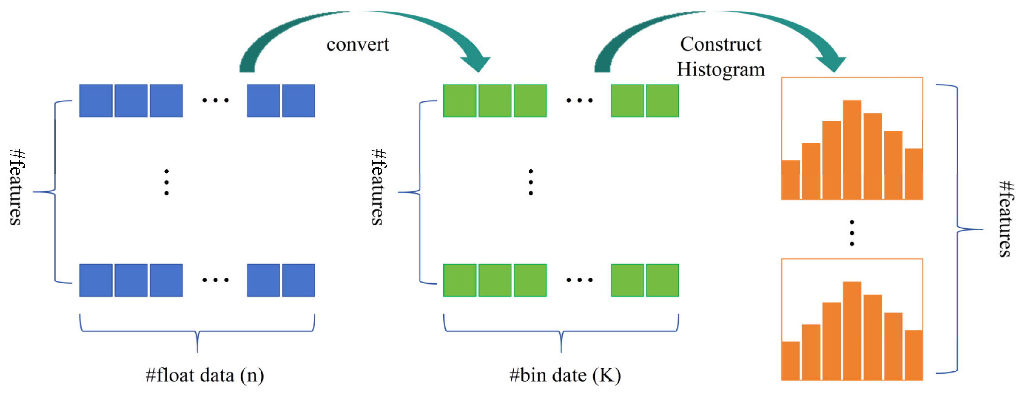
LightGBM uses the histogram algorithm instead of the pre-sorted method. As shown in Figure 8, LightGBM discretizes continuous features into K bins and constructs feature histograms, reducing the complexity of finding split points from O(number of data × number of features) to O(K × number of features). Furthermore, it further accelerates calculations through histogram difference technology—allowing histograms of leaf nodes to be generated by computing the difference between the histograms of parent nodes and sibling nodes, which greatly reduces the amount of computation.

Figure 8. Schematic diagram of the histogram-based algorithm in LightGBM.

2.

Leaf-wise Strategy

As shown in Figure 9, different from the traditional Level-wise strategy, LightGBM adopts the Leaf-wise strategy. Each time, it selects the leaf node with the maximum split gain from all current leaf nodes for splitting. Compared with Level-wise, under the same number of splits, Leaf-wise can reduce errors more effectively. However, it may lead to overfitting; therefore, it is necessary to introduce a maximum depth constraint [40] to balance model complexity and generalization ability.

Figure 9. Schematic diagram of the leaf-wise tree growth strategy in LightGBM.

3.

Gradient-based One-Side Sampling (GOSS)

In GBDT, the magnitude of a sample’s gradient reflects its importance for model training. Samples with small gradients have been well-fitted by the model and contribute little to model updates; in contrast, samples with large gradients are those the model has not yet fully learned and are more important for model updates. Targeting the difference in sample importance, the GOSS algorithm retains samples with large gradients, randomly samples small-gradient samples, and multiplies these sampled small-gradient samples by a weight of ${\displaystyle \frac{1-a}{b}}$ to correct distribution bias [41]. This reduces the amount of computation while maintaining the balance of data distribution.

4.

Exclusive Feature Bundling (EFB)

In practical machine learning tasks, there are often a large number of sparse features, and many of these features are exclusive—meaning they never take non-zero values simultaneously. Leveraging this characteristic, the EFB algorithm bundles exclusive features into a single new feature, thereby reducing the number of features and lowering computational complexity.

3.2. Bayesian Optimization

Bayesian optimization (BO) is a global optimization method based on probabilistic models. Its core idea is to quantify the uncertainty of the objective function through a probabilistic model and combine it with an intelligent sampling strategy to approximate the optimal solution with as few evaluation times as possible [42].

BO mainly consists of three key components:

1.

Surrogate Model

The surrogate model is used to approximate the true objective function $f\left(x\right)$ follows based on previously observed samples. BO assumes that $f\left(x\right)$ follows a certain probability distribution and employs a probabilistic model to capture both the predicted mean and the associated uncertainty. The most commonly used surrogate model is the Gaussian Process (GP), which provides not only an estimate of the function value at unobserved points but also a measure of confidence through its predictive variance. The GP model can be expressed as

$$f(x)~GP(m(x),k(x,x^{\prime }))$$

(20)

where $m\left(x\right)$ is the mean function, $k(x,x^{\prime })$ is the covariance function.

By leveraging the conditional distribution property of GP, the posterior mean and variance can be calculated:

$${\mu }_{*}=k_{*}^T{(K+{\sigma }_n^{2}I)}^{-1}y$$

(21)

$${\sigma }_{*}^2=k(x_{*},x_{*})-k_{*}^T{(K+{\sigma }_n^{2}I)}^{-1}{k}_{*}$$

(22)

where $k_{*}$ is the covariance vector between the new point and the training points, $K$ is the covariance matrix$(K_{ij}=k(x_i,x_j))$.

2.

Acquisition Function

Based on the prediction results of the surrogate model, BO determines the next evaluation point through an Acquisition Function—specifically, the point that maximizes the acquisition function. Acquisition functions are typically functions for which the optimal value is easy to compute, such as the Expected Improvement (EI) function:

$${\alpha }_{\mathrm{EI}}(\mathrm{x})=\left\{\begin{array}{ll}(f(x^{+})-\mu (x))\Phi (Z)+\sigma (x)\varphi (Z)\hfill & \sigma (x)>0\hfill \\ 0\hfill & \sigma (x)=0\hfill \end{array}\right.$$

(23)

where $Z={\displaystyle \frac{f\left(x^{+}\right)-\mu \left(x\right)}{\sigma \left(x\right)}}$, $\mathrm{\Phi }\left(Z\right)$ is the Cumulative Distribution Function, and $\varphi \left(Z\right)$ is the Probability Density Function.

$$\Phi (Z)={\displaystyle {\int }_{-\infty }^Z\frac{1}{\sqrt{2\pi }}}{e}^{-{\displaystyle \frac{t^2}{2}}}dt$$

(24)

$$\varphi (Z)={\displaystyle \frac{1}{\sqrt{2\pi }}}{e}^{-{\displaystyle \frac{Z^2}{2}}}$$

(25)

3.

Iterative Update

At each iteration, the selected point $x_{\mathrm{n}+1}$ is evaluated on the true objective function $f\left(x\right)$, and the resulting value $f\left(x_{\mathrm{n}+1}\right)$, is added to the historical dataset. The surrogate model is then updated, and a new point is selected based on the acquisition function. This iterative cycle continues until the stopping criterion is reached, after which the point yielding the best observed $f\left(x\right)$ is reported.

3.3. BO-LightGBM Data-Driven Model

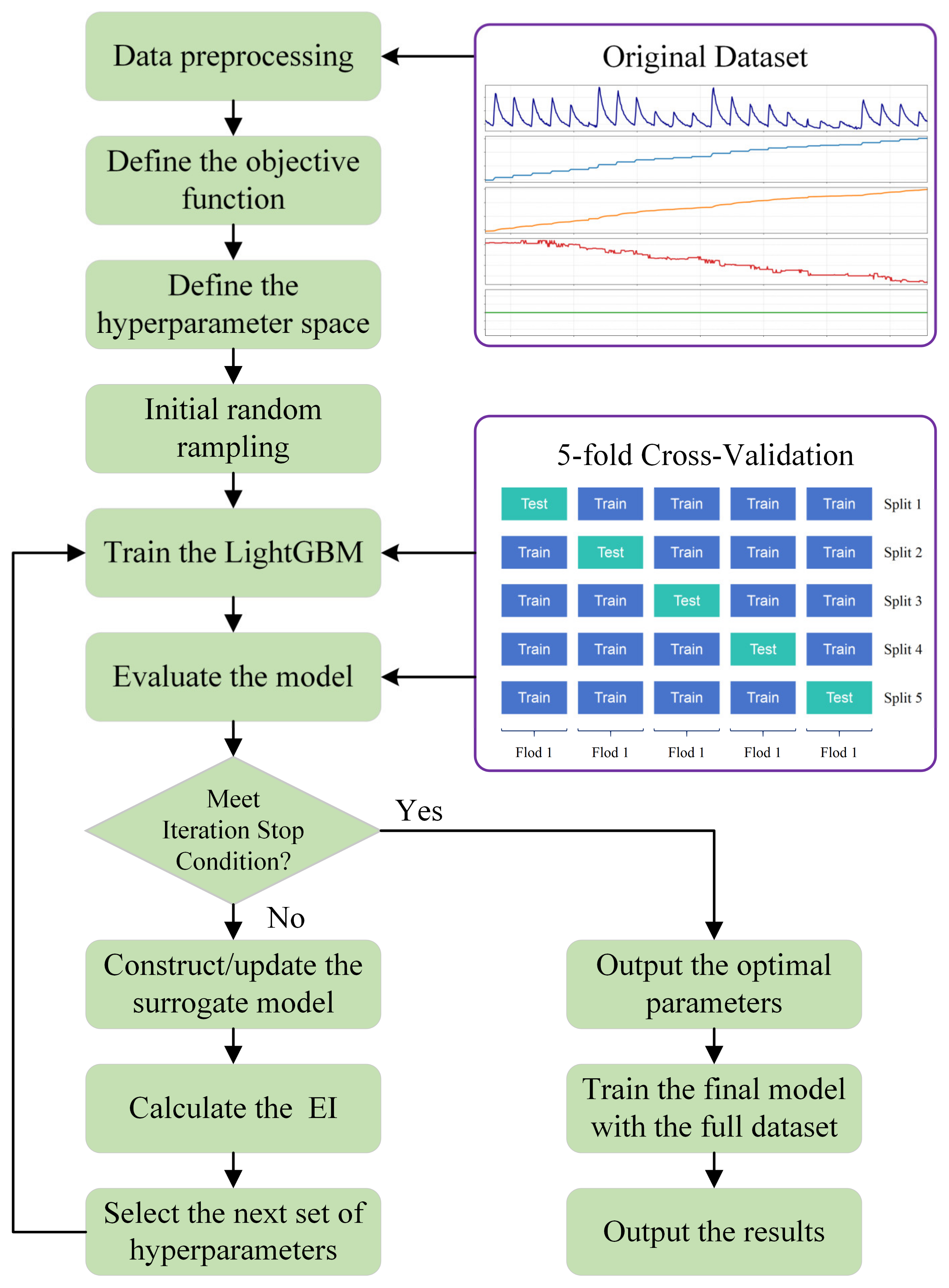
In the construction of machine learning models, the selection of hyperparameters directly affects model performance [43]. Traditional hyperparameter optimization methods (such as grid search and random search) either lead to a sharp increase in computational cost due to exhaustive attempts or suffer from low efficiency due to the lack of utilization of historical information, making it difficult to adapt to the complex parameter space of LightGBM. In contrast, BO can quantify the uncertainty of parameter values by establishing a probabilistic surrogate model of the objective function, and dynamically balance exploration and exploitation based on the acquisition function, thereby efficiently locating the optimal parameter combination within a limited number of iterations. In this paper, Bayesian optimization is employed to adaptively tune the hyperparameters of LightGBM, thereby constructing the BO-LightGBM model for enhanced learning efficiency and prediction accuracy. The model development process is illustrated in Figure 10, and the specific steps are as follows:

Figure 10. Construction process of the BO-LightGBM model.

(1)

First, clean the original data to handle missing values, outliers, and duplicate values in the data; divide the cleaned dataset into a training set and a test set according to the characteristics of time series; construct effective features based on industrial mechanisms as the input variables of the model.

(2)

Based on the characteristics of industrial data and the requirements for model robustness, select the L1 loss as the objective function. The model is validated using 5-Fold Time Series Cross-Validation to simulate real-world application scenarios and avoid evaluation bias caused by data leakage.

(3)

Define the search space for the core hyperparameters of LightGBM, including learning_rate, max_depth, num_leaves, etc.

(4)

Train the LightGBM model based on the hyperparameters generated by initial random sampling to provide initial data for the subsequent construction of the surrogate model.

(5)

Use MAE (Mean Absolute Error) as the core evaluation metric to evaluate the performance of the LightGBM model corresponding to each group of hyperparameters on the validation set. Record the MAE value of the validation set corresponding to each group of hyperparameters to form a historical evaluation dataset of “hyperparameters-performance”.

(6)

Construct/update the surrogate model based on historical evaluation results. Select the next group of hyperparameters that are most likely to improve performance through the EI, and use this group of hyperparameters to train a new LightGBM model.

(7)

Repeat steps 5–6 until the preset stopping condition is met (reaching the maximum number of iterations or convergence of model performance). After terminating the iteration process, output the optimal parameters.

(8)

Retrain the model on the full training set using the optimal parameters to form the final model.

3.4. Cascade–Additive Hybrid Model

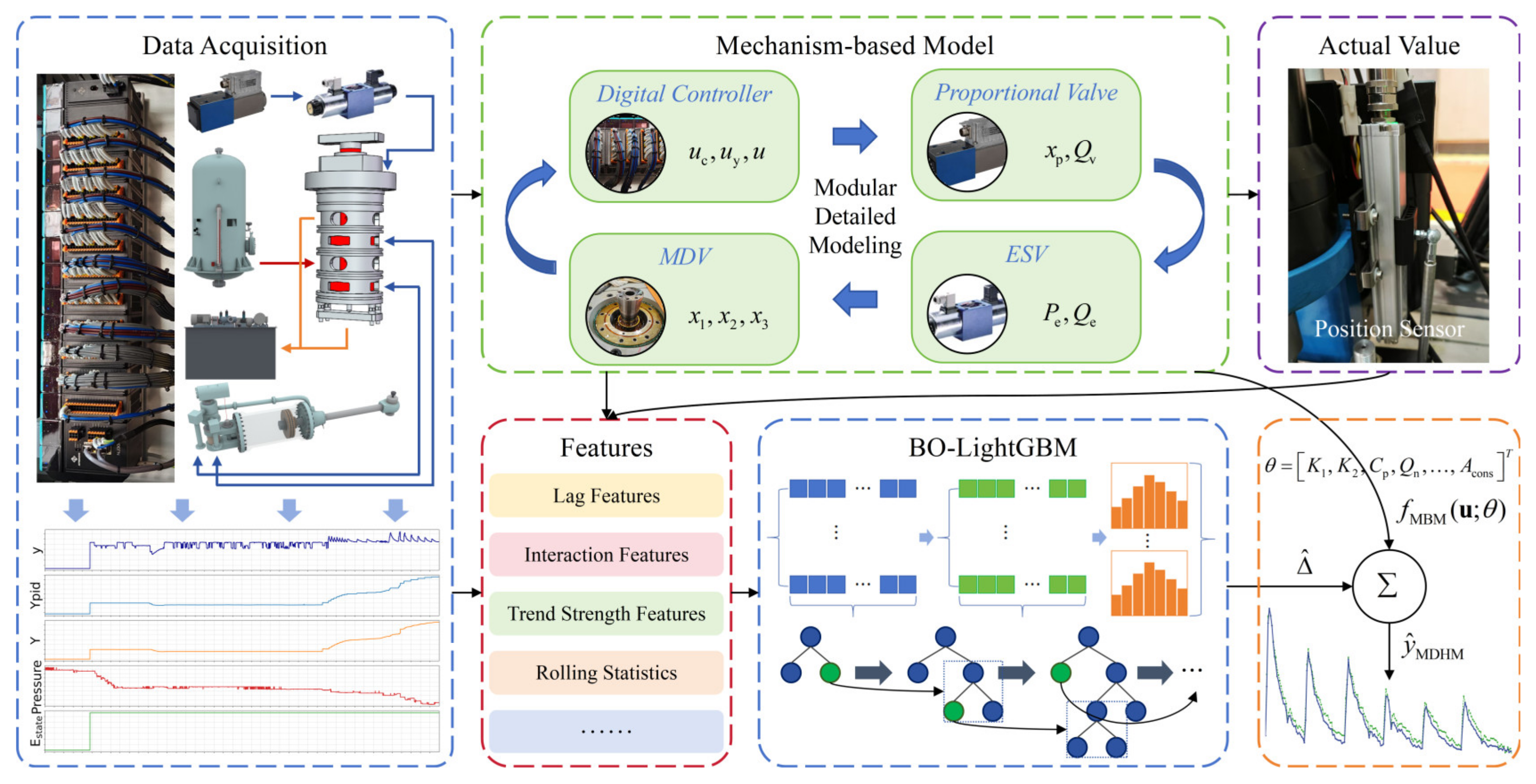
The hybrid architectures integrating mechanism-based and data-driven models can generally be categorized into three representative forms: Series architecture [44], Parallel architecture [45], and embedded architecture [46]. Given the high physical clarity of the MBM developed in this study, a cascade–additive hybrid strategy, regarded as an enhanced form of the series architecture, is adopted to strengthen the synergy between the mechanistic and data-driven components, accurately capture operation-specific error patterns—namely, regions where the MBM exhibits notably increased prediction errors under certain operating conditions—and ensure the physical interpretability and traceability of the simulation results. On this basis, a mechanistic–data-driven hybrid model (MDHM) is developed for the MDV position, as illustrated in Figure 11.

Figure 11. Cascade–additive, mechanistic–data-driven hybrid architecture.

Four types of data—the hydraulic pressure of the pressure tank, the guide vane control output, the guide vane opening, and the ESV state—are used as input variables for the MBM to obtain a preliminary estimate of the MDV position. The deviation between the MBM outputs and the actual measurements characterizes the complex dynamic characteristics and uncertainties that cannot be explained by the MBM:

$${\Delta }_i=y_i-f_{\mathrm{MBM}}(u_i;\theta )$$

(26)

where $y_i$ is the actual value of the i-th sample, $f_{\mathrm{M}\mathrm{B}\mathrm{M}}(u_i,\theta )$ represents the MBM output of the i-th sample, $u_i$ is the input vector of the i-th sample, and $\theta$ denotes the parameter vector of the MBM.

To further improve the overall model accuracy, the BO-LightGBM model is introduced on the physical basis of the MBM to specifically learn the deviation, dynamically capturing the unmodeled dynamics and system uncertainties. The input features used in the BO-LightGBM model consist of original time-series features, the output of the MBM, and their derived features, as summarized in Table 1. The original features provide basic information on system inputs, while interaction features—constructed from combinations of original features—capture nonlinear dependencies between variables. Lag and rolling features account for system inertia, delayed effects, and short-term dynamic trends. The MBM output serves as a physical baseline, allowing the model to focus on residual errors, and trend strength features quantify the persistence and intensity of dynamic trends, capturing cumulative effects. Together, this feature set enables the BO-LightGBM model to efficiently learn unmodeled dynamics and system uncertainties, complementing the mechanistic knowledge provided by the MBM.

Table 1. Input features of the data-driven model.

Feature Type	Feature Name
Original features	Pressure of the pressure tank
	Guide vane control output
	Guide Vane Opening
	ESV state
MBM output	MBM-simulated position
Interaction features	Opening deviation
Lag features	Opening deviation-lag
	MBM-simulated position-lag
	MBM simulation deviation-lag
Trend strength features	Opening deviation-trend strength
	MBM-simulated position-trend strength
Rolling mean	Opening deviation-rolling mean
	MBM-simulated position-rolling mean
	MBM simulation deviation-rolling mean
Rolling maximum	Opening deviation-rolling max
	MBM-simulated position-rolling max
	MBM simulation deviation-rolling max
Rolling standard deviation	Opening deviation-rolling Std
	MBM-simulated position-rolling Std
	MBM simulation deviation-rolling Std

Finally, by additively combining the mechanistic simulation result and the learned compensation term, the final simulated output of the MDHM is obtained as

$${\widehat{y}}_i=f_{\mathrm{MBM}}(u_i;\theta )+{\widehat{\Delta }}_i$$

(27)

where ${\widehat{∆}}_i$ represents the compensation generated by the BO-LightGBM for the i-th sample.

4. Case Study and Result Analysis

4.1. Data Preparation and Model Parameterization

4.1.1. Data Preparation

The data used in this study were obtained from the governor of a large hydropower plant, including oil pressure of the pressure tank, guide vane control output, guide vane opening, ESV state, and MDV position, with a sampling interval of 0.2 s. The dataset covers three typical operating scenarios—start-up, shutdown, and load regulation—as well as one extreme scenario, namely load rejection. Prior to modeling, the data were carefully preprocessed: outliers and missing values were identified and removed, and physically implausible measurements were corrected to ensure data quality. Following this cleaning procedure, a total of 23,293 valid samples were obtained. For constructing the data-driven model, the dataset was divided into a training set and a test set at a ratio of 7:3, and 5-fold cross-validation was performed within the training set.

4.1.2. Parameter Configuration of the MBM

Based on the characteristics of the parameters and their actual availability, this paper comprehensively adopts multiple methods, such as experimental determination, consulting design data, and empirical value estimation, to determine the values of the core parameters of the MBM. The detailed parameter configuration is presented in Table 2. Due to confidentiality requirements, only representative mechanistic parameters are presented, while several sensitive parameters are not disclosed but were used consistently in the modeling and validation to ensure the reliability of the results.

Table 2. Core parameters of the MBM.

Parameter	Symbol	Value	Description
Large-loop gain coefficient	$K_1$	3	Tuning value
Small-loop gain coefficient	$K_2$	0.3	Tuning value
Positive compensation coefficient	$C_{\mathrm{p}}$	-	Confidential
Negative compensation coefficient	$C_1$	-	Confidential
Gain coefficient (second-order system)	$K$	1	Derived from the Bode diagram
Natural frequency (second-order system)	$\zeta$	326.7 rad/s	Derived from the Bode diagram
Damping ratio (second-order system)	${\omega }_n$	0.6	Derived from the Bode diagram
Return oil pressure	$P_{\mathrm{t}}$	5 bar	Empirical value
Rated flow of the proportional valve	$Q_n$	40 min/L	Obtained from the product manual
Density of hydraulic oil	$\rho$	880 kg/m3	Typical density of No. 46 hydraulic oil
Bulk modulus of hydraulic oil	$\beta$	1500 Mpa	Selected from the typical range
Mass of the MDV spool	$m$	-	Confidential
Self-centering spring stiffness	$k$	7453 N/m	Experimentally measured
Viscous damping coefficient	$B$	5000 N·s/m	Selected from the typical range
Lower limit of MDV spool position	$x_{\mathrm{m}\mathrm{i}\mathrm{n}}$	−18.80%	Normalized with respect to rated value
Upper limit of MDV spool position	$x_{\mathrm{m}\mathrm{a}\mathrm{x}}$	12.05%	Normalized with respect to rated value
Control chamber area	$A_{\mathrm{c}\mathrm{t}\mathrm{r}\mathrm{l}}$	-	Confidential
Constant-pressure chamber area	$A_{\mathrm{c}\mathrm{o}\mathrm{n}\mathrm{s}}$	-	Confidential

Preliminary variation tests and physical reasoning indicate that uncertainties in the empirically determined parameters primarily affect the MBM output, while their impact on the final hybrid model is limited, as the BO-LightGBM module compensates for residual dynamics.

4.1.3. Hyperparameter Optimization of the BO-LightGBM

Bayesian optimization was employed to perform hyperparameter tuning for improved model performance. The maximum number of iterations was set to 50 to achieve a trade-off between optimization accuracy and computational cost. The hyperparameter search space covered three key dimensions relevant to LightGBM performance: (i) model complexity, controlling the depth and number of trees and thus affects the model’s capacity to fit nonlinear relationships; (ii) regularization parameters, constraining model complexity and mitigate overfitting, ensuring good generalization across diverse operating conditions; and (iii) sampling strategies, enhancing robustness through introducing randomness during tree construction. The specific parameter ranges and tuning results are summarized in Table 3.

Table 3. Hyperparameter search ranges and optimal results.

Hyperparameter	Description	Search Range	Optimal Value
learning_rate	Step size shrinkage	0.001–0.1	0.022
num_leaves	Maximum number of leaves in one tree	20–300	161
max_depth	Maximum depth of a tree	3–25	17
min_data_in_leaf	Minimum number of data points in a leaf	10–100	33
lambda_l1	L1 regularization coefficient	0–10	10
lambda_l2	L2 regularization coefficient	0–10	3.475
feature_fraction	Fraction of features used for each tree	0.5–1	0.642
bagging_fraction	Fraction of data used for each iteration	0.5–1	1
bagging_freq	Frequency of performing bagging	0–10	3

4.2. Results and Discussion

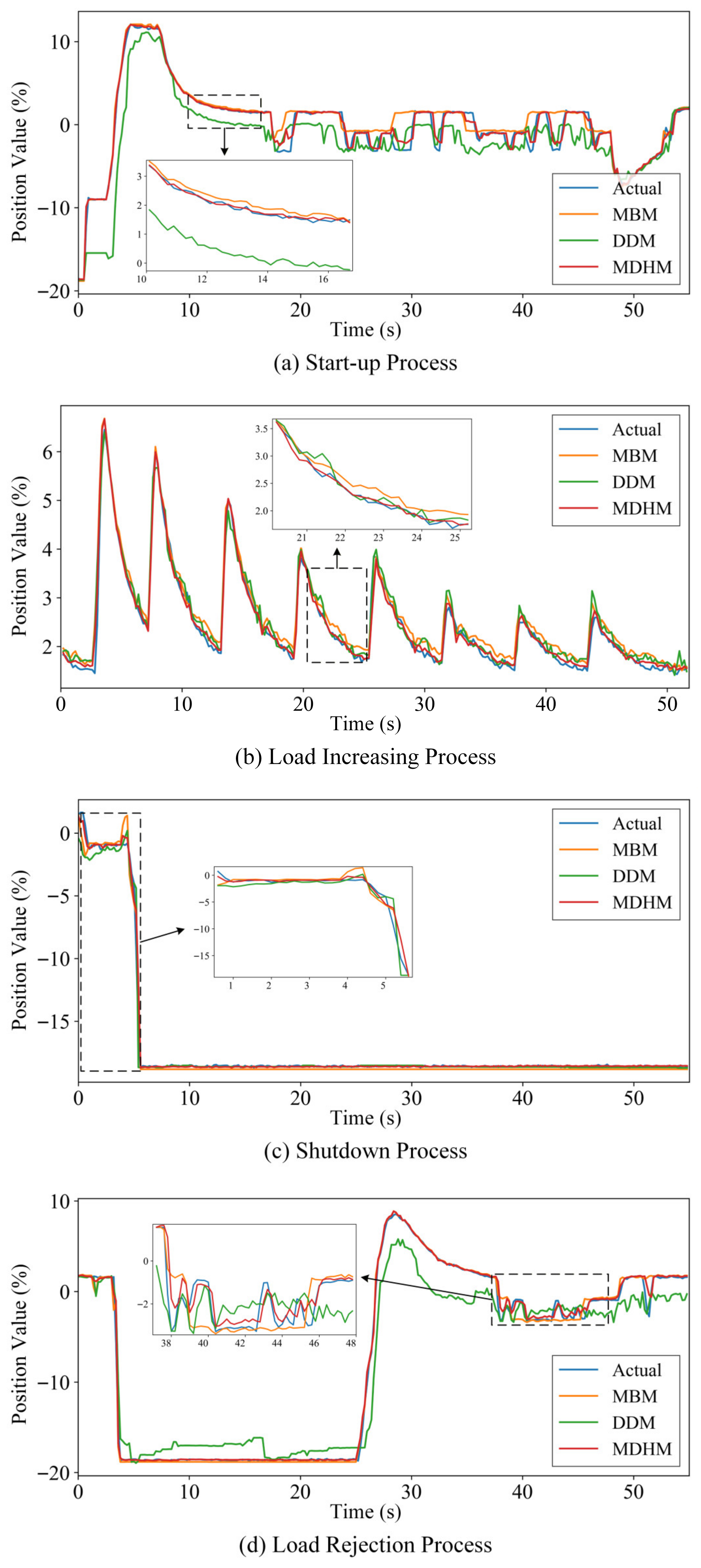
To verify the effectiveness of the proposed MDHM, tests were conducted under four dynamic operating conditions, including startup, load increasing, shutdown, and load rejection. The model is also compared with the MDM and standalone data-driven model (DDM). The simulation results of different models under these dynamic processes are shown in Figure 12.

Figure 12. Comparison of models under four dynamic processes.

For a comprehensive evaluation of the model performance, three commonly used indicators, namely the Mean Absolute Error (MAE), Root Mean Square Error (RMSE), and Coefficient of Determination (R²), were adopted. The formulas are expressed as follows:

$$MAE={\displaystyle \frac{1}{n}}{\displaystyle \sum _{i=1}^n\left|y_i-{\widehat{y}}_i\right|}$$

(28)

$$RMSE=\sqrt{{\displaystyle \frac{1}{n}}{\displaystyle \sum _{i=1}^n{(y_i-{\widehat{y}}_i)}^2}}$$

(29)

$$R^2=1-{\displaystyle \frac{{\displaystyle \sum _{i=1}^n{(y_i-{\widehat{y}}_i)}^2}}{{\displaystyle \sum _{i=1}^n{(y_i-\overline{y})}^2}}}$$

(30)

where $y_i$ and ${\widehat{y}}_i$ denote the actual and simulated values, respectively, $n$ is the number of samples, and $\overline{y}$ represents the mean of the actual values.

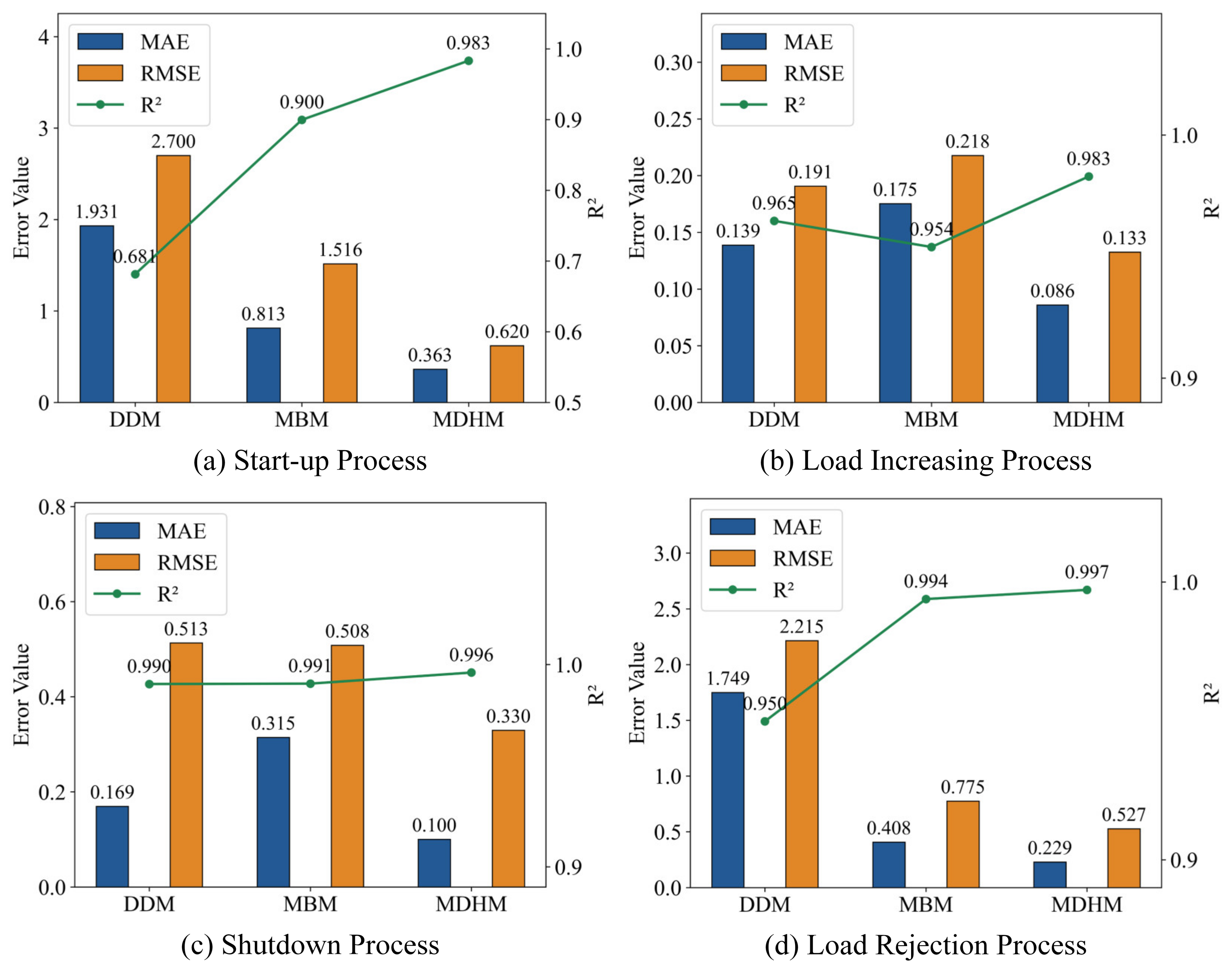
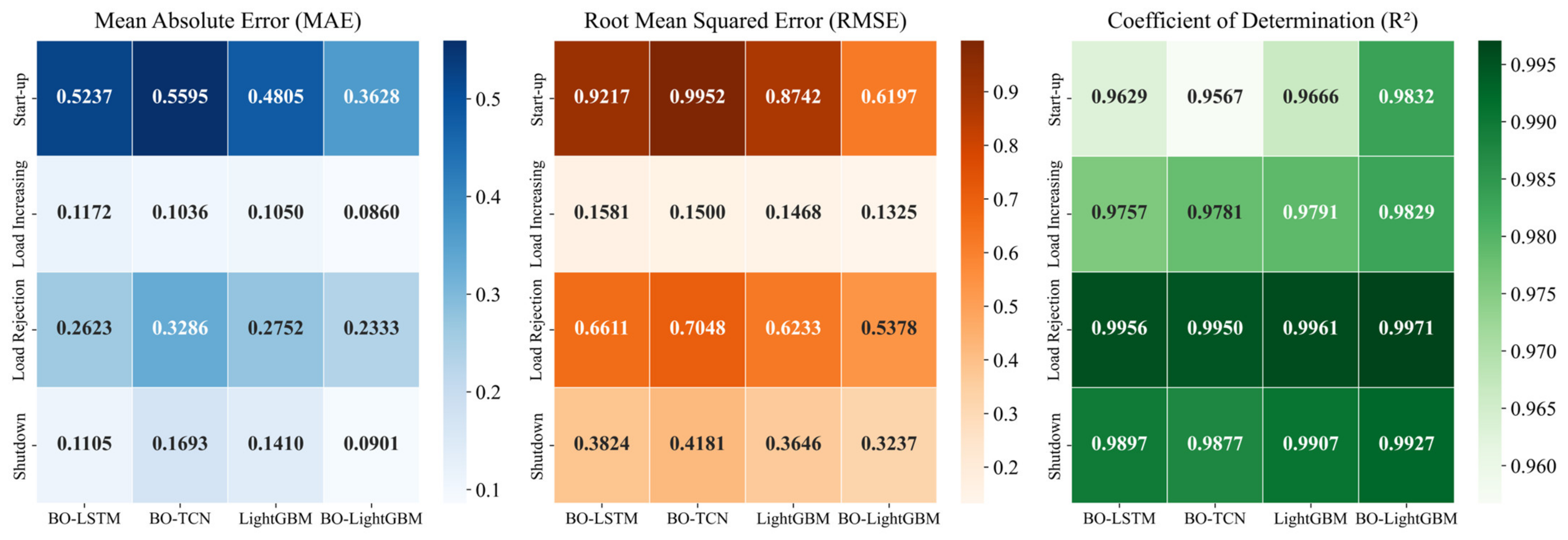
The computed results of these metrics are presented in Figure 13.

Figure 13. Comparison of model performance based on MAE, RMSE, and R² metrics.

The results show that the MDM can generally reflect the main motion characteristics and dynamic response trends of the MDV spool, and exhibits good stability within a certain range. However, its simulation results still present considerable deviations. In particular, the model performance degrades significantly within the range of −3.5% to 2%. This is mainly because many parameters in the mechanistic model (e.g., damping coefficients) are difficult to determine accurately, often relying on empirical settings or offline identification, and because some influencing factors are simplified or neglected during the modeling process.

The DDM performs well during the load-increasing process; however, it exhibits limited stability, especially during the startup and load-rejection processes, where the deviations between the simulated and actual values are relatively large, resulting in unsatisfactory overall performance. This phenomenon arises primarily from the model’s strong dependence on training samples—its learning process is constrained by both the quantity of available data and the biased coverage of specific operating conditions (e.g., load increase) within the training dataset.

Across all test conditions, the MDHM demonstrates the best overall performance, with an average R² as high as 0.990 and no performance degradation observed under any dynamic process. Compared with the MDM and DDM, the MAE of the MDHM is reduced by 43.9–68.3% and 38.1–86.9%, respectively, while the RMSE decreases by 32.0–59.1% and 30.4–77.0%, respectively. Notably, the advantages of the MDHM are not confined to any specific operating condition, which stands in sharp contrast to the DDM—whose MAE increases sharply during the start-up and load rejection processes despite acceptable performance in load increasing and shutdown scenarios—and the MDM, which performs only moderately across all dynamic processes. These results indicate that the proposed hybrid model effectively integrates the strengths of both mechanistic and data-driven approaches, significantly enhancing stability and simulation accuracy, and making it more suitable for complex and variable real-world operating conditions.

4.3. Verification of the Superiority of the BO-LightGBM

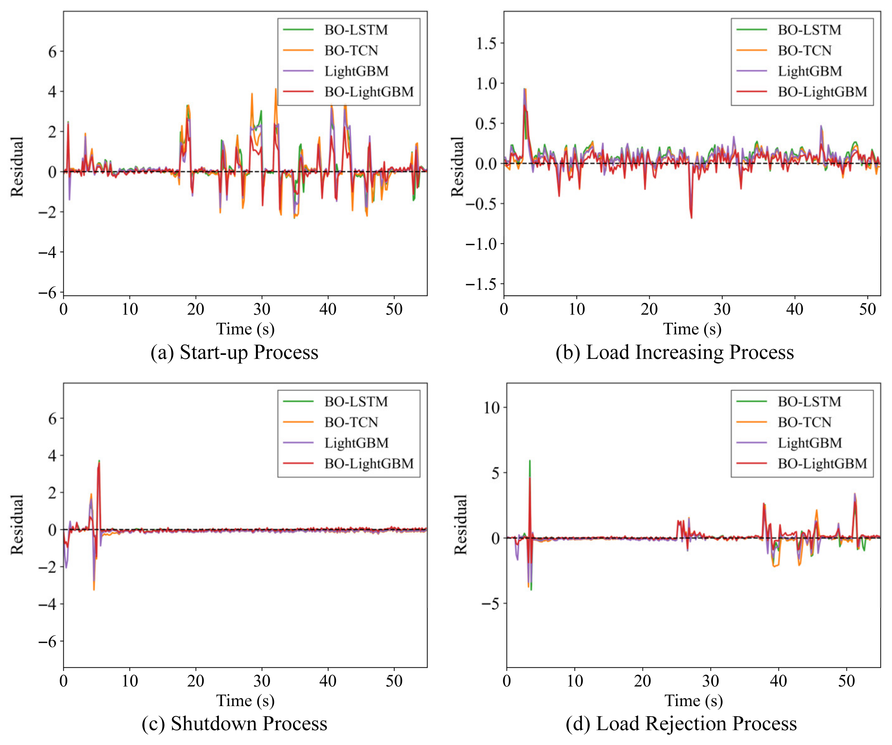
To further verify the effectiveness of the proposed BO-LightGBM, three data-driven models were selected for comparison: a manually tuned LightGBM, a BO-optimized LSTM (BO-LSTM), and a BO-optimized Temporal Convolutional Network (BO-TCN). Using the training dataset described in Section 4.1, hybrid models were constructed with each method under the same input features and evaluation metrics. Their performance was evaluated on an identical test dataset. Figure 14 shows the residual comparison of different models, defined as the differences between simulated and actual values.

Figure 14. Comparison of residuals for different models.

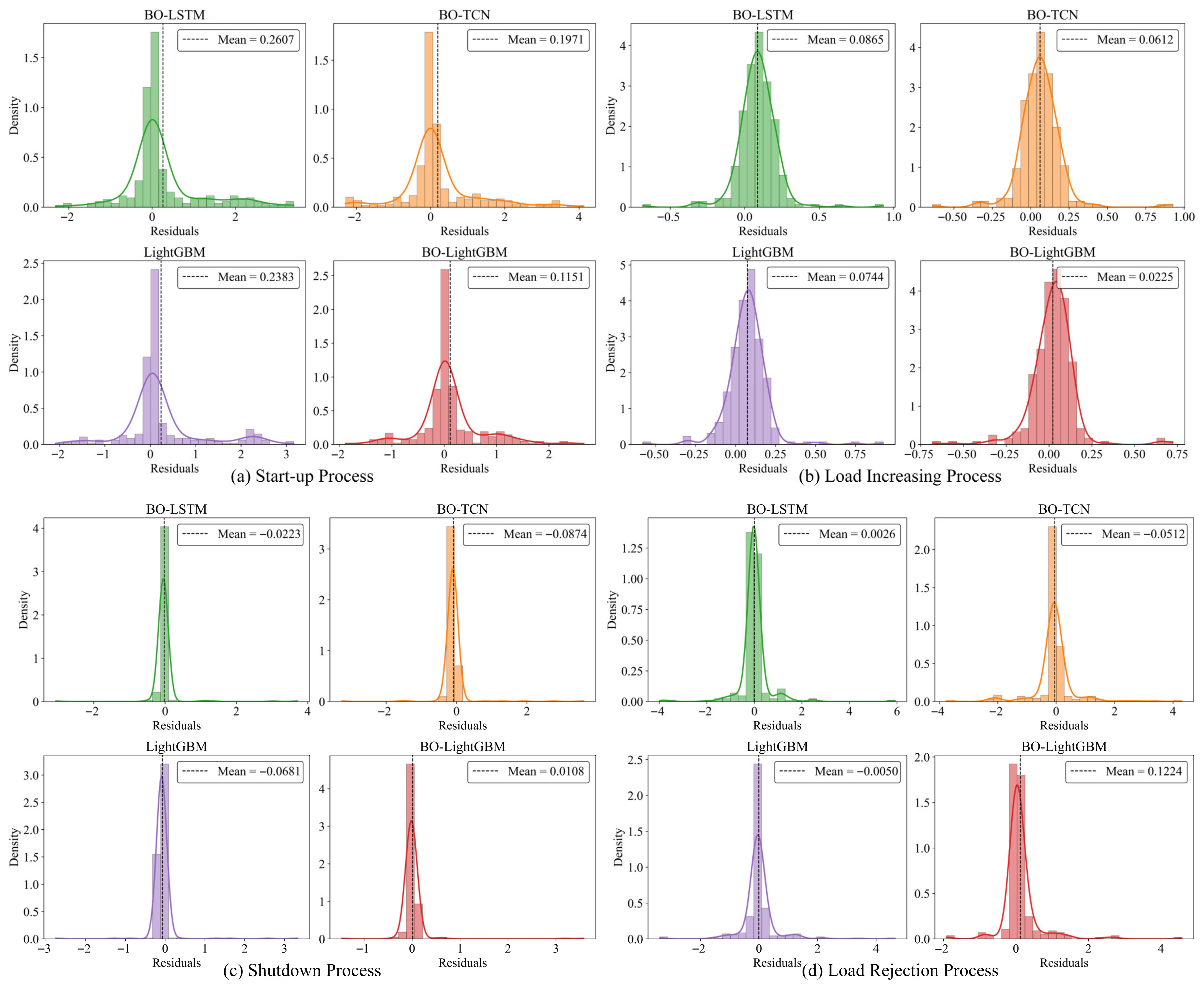
Figure 15 further presents the residual distribution of each hybrid model in the form of histograms with kernel density estimation (KDE). From this figure, it can be observed that during the start-up, load increasing, and shutdown processes, the residual distribution of the hybrid model based on BO-LightGBM is closest to the ideal state, characterized by a mean value approaching zero and small fluctuations, indicating that it performs best under these three operating conditions. Under extreme conditions such as load rejection, the model tends to slightly overestimate the results; however, the deviations are minor, and most residuals remain concentrated around zero. In contrast, other models exhibit wider residual distributions, indicating that the BO-LightGBM hybrid model possesses superior stability.

Figure 15. Histogram with KDE of residuals.

Figure 16 presents a heatmap summarizing the performance metrics of different hybrid models under various operating conditions. It can be observed that the BO-LightGBM hybrid model performs best across all operating conditions, and the overall performance ranking of the hybrid models is as follows: BO-LightGBM > LightGBM > BO-LSTM > BO-TCN. This ranking can be explained as follows. LightGBM inherently has an advantage in handling structured tabular data, and the “multivariable coupling” characteristics of industrial time-series data are well aligned with the “multi-feature fusion mechanism” of LightGBM. Furthermore, Bayesian optimization, through Gaussian process modeling and the expected improvement criterion, efficiently explores the hyperparameter space and identifies the optimal parameter combinations suited to the current task.

Figure 16. Performance metrics heatmap of different hybrid models.

Although BO-LSTM specifically models time-series dependencies through its internal gating mechanism, its performance is slightly inferior to that of LightGBM. This is because the long-term complex dependencies in the data are not significant, and it may also be due to the fact that the existing data scale fails to fully stimulate the deep time-series modeling potential of the LSTM network. BO-TCN, on the other hand, extracts temporal features through causal and dilated convolutions. However, its fixed convolutional mechanism does not align well with the non-stationary and dynamically dependent characteristics of industrial time-series data, resulting in lower overall accuracy.

In summary, the above results demonstrate from multiple perspectives the effectiveness and superiority of the BO-LightGBM hybrid model in the task of simulating the position of the MDV.

5. Conclusions and Future Work

In this paper, a mechanistic–data-driven hybrid modeling approach is proposed to accurately simulate the dynamic response process of the MDV. The main research conclusions are as follows:

(1)

By in-depth exploration of the internal operating principles of the governor’s servo system, a nonlinear MBM was constructed. This model comprehensively characterizes the spool’s key motion features and dynamic response behavior, demonstrating good stability under complex dynamic conditions and providing a solid physical foundation for subsequent hybrid modeling.

(2)

A BO-LightGBM model was proposed to specifically learn the complex behaviors and uncertainties that cannot be captured by the MBM. Through a cascade–additive hybrid framework, the method achieves complementary advantages between physical prior knowledge and data-driven learning capability, significantly improving prediction accuracy without compromising physical interpretability.

(3)

The effectiveness and superiority of the proposed hybrid model were validated through comparative experiments under multiple operating conditions. The hybrid model demonstrated the best performance across the three tested typical dynamic processes and one extreme condition, achieving maximum MAE reductions of 68.3% and 86.9% compared with the mechanism-based and data-driven models, respectively. Further comparison results indicate that employing BO-LightGBM as the data-driven module in the hybrid framework yields higher accuracy and stability in simulating the MDV position.

The proposed model in this study is custom-developed around the core scenario of a digital twin system, aiming to accurately replicate the individual characteristics of a specific MDV. It effectively addresses the limitations of traditional models under nonlinear and time-varying operating conditions while maintaining good generalizability for broader applications.

Future research will focus on three main directions: (1) Investigating deeper mechanism–data fusion strategies and exploring more dynamically interactive fusion frameworks. (2) Incorporating uncertainty quantification into the hybrid modeling framework, for example, by exploiting the probabilistic characteristics of the Bayesian optimization surrogate model or by introducing techniques such as quantile regression or ensemble-based uncertainty estimation within the data-driven component. Enhancing the model with uncertainty information will enable risk-aware prediction and further improve the reliability of digital-twin applications in safety-critical hydropower scenarios. (3) Establishing adaptive learning mechanisms that enable the model to dynamically adjust to equipment aging, operational drifts, and evolving system behaviors over time, thereby ensuring sustained accuracy, robustness, and responsiveness in digital twin implementations.

References

1. Ellabban, O.; Abu-Rub, H.; Blaabjerg, F. Renewable energy resources: Current status, future prospects and their enabling technology. Renew. Sustain. Energy Rev. 2014, 39, 748–764. [Google Scholar] [CrossRef]
2. Shu, Y.; Chen, G.; He, J.; Zhang, F. Building a New Electric Power System Based on New Energy Sources. Strateg. Study CAE 2021, 23, 61–69. [Google Scholar] [CrossRef]
3. Xu, B.B.; Zhang, J.J.; Egusquiza, M.; Chen, D.Y.; Li, F.; Behrens, P.; Egusquiza, E. A review of dynamic models and stability analysis for a hydro-turbine governing system. Renew. Sustain. Energy Rev. 2021, 144, 110880. [Google Scholar] [CrossRef]
4. Yang, W.J.; Norrlund, P.; Bladh, J.; Yang, J.D.; Lundin, U. Hydraulic damping mechanism of low frequency oscillations in power systems: Quantitative analysis using a nonlinear model of hydropower plants. Appl. Energy 2018, 212, 1138–1152. [Google Scholar] [CrossRef]
5. Mitchell, C. Momentum is increasing towards a flexible electricity system based on renewables. Nat. Energy 2016, 1, 6. [Google Scholar] [CrossRef]
6. Chang, M.K.; Eichman, J.D.; Mueller, F.; Samuelsen, S. Buffering intermittent renewable power with hydroelectric generation: A case study in California. Appl. Energy 2013, 112, 1–11. [Google Scholar] [CrossRef]
7. Kumari, R.; Prabhakaran, K.K.; Desingu, K.; Chelliah, T.R.; Sarma, S.V.A. Improved Hydroturbine Control and Future Prospects of Variable Speed Hydropower Plant. IEEE Trans. Ind. Appl. 2021, 57, 941–952. [Google Scholar] [CrossRef]
8. Zhang, N. Study on Nonlinear Model Parameter Identification and Control Optimization of Pumped Storage Unit Governing System. Ph.D. Thesis, Huazhong University of Science and Technology, Wuhan, China, 2019. [Google Scholar]
9. Wu, J.; Zhou, B.; Li, Z.; He, L.; Xu, D. Static Characteristic Simulations of Giant Main Distributing Valve. Hydropower Pumped Storage 2012, 36, 24–26. [Google Scholar]
10. Liu, H.; Chang, Z.; Lu, Z.; Pi, C.; Yang, G. Technical Modification of Displacement Sensor for Main Distribution Valve of Governor in Xiangjiaba Hydropower Plant. China Rural Water Hydropower 2020, 138–142. Available online: https://irrigate.whu.edu.cn/EN/Y2020/V0/I2/138 (accessed on 25 September 2025).
11. Tu, Y.; Zhang, Q. Research on intelligent diagnosis method of governor hydraulic tracking fault. Yangtze River 2022, 53, 184–187. [Google Scholar] [CrossRef]
12. Calinoiu, C.; Vasiliu, D.; Radu, P.; Vasiliu, N.; Cristinel, I.P. Sizing and tuning speed governors for turbines by AMESIM. In Proceedings of the European Simulation and Modelling Conference (ESM 2013), Lancaster University, Lancaster, UK, 23–25 October 2013; pp. 220–226. [Google Scholar]
13. Fang, H.Q.; Chen, L.; Dlakavu, N.; Shen, Z.Y. Basic Modeling and simulation tool for analysis of hydraulic transients in hydroelectric power plants. IEEE Trans. Energy Convers. 2008, 23, 834–841. [Google Scholar] [CrossRef]
14. Tian, Y.Q.; Wang, B.; Chen, P.; Yang, Y. Finite-time Takagi-Sugeno fuzzy controller design for hydraulic turbine governing systems with mechanical time delays. Renew. Energy 2021, 173, 614–624. [Google Scholar] [CrossRef]
15. Li, C.S.; Zhou, J.Z.; Xiao, J.; Xiao, H. Hydraulic turbine governing system identification using T S fuzzy model optimized by chaotic gravitational search algorithm. Eng. Appl. Artif. Intell. 2013, 26, 2073–2082. [Google Scholar] [CrossRef]
16. Lu, X.D.; Li, C.S.; Chang, H.; Wang, H.; Zhu, Z.W.; Liu, D.; Tan, X.Q.; Xu, R.L. Primary frequency regulation performance in hydropower systems: Precise quantification and holistic enhancement under wide-range operation. Appl. Energy 2025, 389, 21. [Google Scholar] [CrossRef]
17. Xiao, Y.; Liu, W.; Wang, G.; Xia, C.; Li, Z.; Yu, D.; Ma, C. Source-grid Coordination of Hydraulic Turbine Governing System. Power Syst. Technol. 2021, 45, 1852–1861. [Google Scholar] [CrossRef]
18. Zhou, B.; Wu, J.; Shao, B. Main Distributing Valve Linear Modeling and Performance Analysis. Water Sci. Eng. Technol. 2014, 25–27. [Google Scholar] [CrossRef]
19. Wu, J.; Su, Y.; Zhang, J.; Zhu, R.; Yu, H. Simulation on the Response Speed of Main Distributing Valve. Hydraul. Pneum. Seals 2013, 33, 30–32. [Google Scholar] [CrossRef]
20. Xia, L.; Wang, Y.; Liu, M.; Jie, S. Simulation and analysis of faults in the electro-hydraulic servo system of hydraulic turbine governor based on SimHydraulics. China Meas. Test 2022, 48, 105–112. [Google Scholar]
21. Yan, N.; Feng, C.; Huang, C. Modeling and Identification Method of Electro-hydraulic Servo System for Hydro Turbine Governor. Water Resour. Power 2019, 37, 166–169+82. [Google Scholar] [CrossRef]
22. Milic, V.; Situm, Z.; Essert, M. Robust H∞ position control synthesis of an electro-hydraulic servo system. ISA Trans. 2010, 49, 535–542. [Google Scholar] [CrossRef]
23. Stosiak, M.; Karpenko, M.; Ivannikova, V.; Maskeliunaite, L. The impact of mechanical vibrations on pressure pulsation, considering the nonlinearity of the hydraulic valve. J. Low Freq. Noise Vib. Act. Control 2025, 44, 706–719. [Google Scholar] [CrossRef]
24. Wu, W.; Wei, C.H.; Zhou, J.J.; Hu, J.B.; Yuan, S.H. Numerical and experimental nonlinear dynamics of a proportional pressure-regulating valve. Nonlinear Dyn. 2021, 103, 1415–1425. [Google Scholar] [CrossRef]
25. Yao, J.Y. Model-based nonlinear control of hydraulic servo systems: Challenges, developments and perspectives. Front. Mech. Eng. 2018, 13, 179–210. [Google Scholar] [CrossRef]
26. Wang, Q.; Li, F.; Tang, Y.; Xu, Y. Integrating Model-Driven and Data-Driven Methods for Power System Frequency Stability Assessment and Control. IEEE Trans. Power Syst. 2019, 34, 4557–4568. [Google Scholar] [CrossRef]
27. Song, H.D.; Liu, X.J.; Song, M.Q. Comparative study of data-driven and model-driven approaches in prediction of nuclear power plants operating parameters. Appl. Energy 2023, 341, 14. [Google Scholar] [CrossRef]
28. Luo, W.C.; Hu, T.L.; Ye, Y.X.; Zhang, C.R.; Wei, Y.L. A hybrid predictive maintenance approach for CNC machine tool driven by Digital Twin. Robot. Comput.-Integr. Manuf. 2020, 65, 16. [Google Scholar] [CrossRef]
29. Guo, Y.H.; Wang, N.B.; Shao, S.Q.; Huang, C.Q.; Zhang, Z.T.; Li, X.Q.; Wang, Y.D. A review on hybrid physics and data-driven modeling methods applied in air source heat pump systems for energy efficiency improvement. Renew. Sustain. Energy Rev. 2024, 204, 14. [Google Scholar] [CrossRef]
30. Li, F.; Wang, Q.; Hu, J.; Tang, Y. Combined Data-driven and Knowledge-driven Methodology Research Advances and Its Applied Prospect in Power Systems. Proc. CSEE 2021, 41, 4377–4390. [Google Scholar] [CrossRef]
31. Zhang, Z.Y.; Wang, H.; Tang, M.; Zhang, J.; Hu, X.H. Hybrid mechanism and data driven approach for high-precision modeling of gas flow regulation systems of VFDR. Complex Intell. Syst. 2025, 11, 23. [Google Scholar] [CrossRef]
32. Tian, H.; Zhao, H.R.; Liu, C.Y.; Chen, J.; Wu, Q.W.; Terzija, V. A dual-driven linear modeling approach for multiple energy flow calculation in electricity-heat system. Appl. Energy 2022, 314, 16. [Google Scholar] [CrossRef]
33. Wang, Z.; Zhu, T.; Chen, Z.; Xi, B.; Jia, X. Design of mechanical structure and hydraulic system of tubular turbine governor. Chin. J. Eng. Des. 2020, 27, 753–764. [Google Scholar] [CrossRef]
34. Kosek, M.; Downar, D.; Sliwinski, P. Hydraulic valve design methodology for hydro turbine control system. Flow Meas. Instrum. 2024, 100, 14. [Google Scholar] [CrossRef]
35. Kosek, M.; Sliwinski, P. Shaping the flow characteristics of a proportional directional valve. Sci. Rep. 2025, 15, 24. [Google Scholar] [CrossRef] [PubMed]
36. Chen, L.; Zhang, C.; Jin, B.; Yuan, T.B. Simulation and experimental research on steady flow force compensation for a servo proportional valve. Flow Meas. Instrum. 2023, 94, 102457. [Google Scholar] [CrossRef]
37. Li, R.C.; Sun, Y.H.; Wu, X.W.; Zhang, P.; Li, D.F.; Lin, J.H.; Xia, Y.H.; Sun, Q.Y. Review of the Research on and Optimization of the Flow Force of Hydraulic Spool Valves. Processes 2023, 11, 2183. [Google Scholar] [CrossRef]
38. Cristofori, D.; Vacca, A. The Modeling of Electrohydraulic Proportional Valves. J. Dyn. Syst. Meas. Control-Trans. Asme 2012, 134, 021008. [Google Scholar] [CrossRef]
39. Ke, G.L.; Meng, Q.; Finley, T.; Wang, T.F.; Chen, W.; Ma, W.D.; Ye, Q.W.; Liu, T.Y. LightGBM: A Highly Efficient Gradient Boosting Decision Tree. In Proceedings of the 31st Annual Conference on Neural Information Processing Systems (NIPS), Long Beach, CA, USA, 4–9 December 2017. Advances in Neural Information Processing Systems 30 (NIPS 2017). [Google Scholar]
40. González, S.; García, S.; Del Ser, J.; Rokach, L.; Herrera, F. A practical tutorial on bagging and boosting based ensembles for machine learning: Algorithms, software tools, performance study, practical perspectives and opportunities. Inf. Fusion 2020, 64, 205–237. [Google Scholar] [CrossRef]
41. Bentéjac, C.; Csörgo, A.; Martínez-Muñoz, G. A comparative analysis of gradient boosting algorithms. Artif. Intell. Rev. 2021, 54, 1937–1967. [Google Scholar] [CrossRef]
42. Shahriari, B.; Swersky, K.; Wang, Z.Y.; Adams, R.P.; de Freitas, N. Taking the Human Out of the Loop: A Review of Bayesian Optimization. Proc. IEEE 2016, 104, 148–175. [Google Scholar] [CrossRef]
43. Yang, L.; Shami, A. On hyperparameter optimization of machine learning algorithms: Theory and practice. Neurocomputing 2020, 415, 295–316. [Google Scholar] [CrossRef]
44. Cheng, C.H.; Huang, K.K.; Zhou, C.; Li, Y.G. Series Dynamic Hybrid Model Based on Material Conservation and Neural Networks for Oxidation Leaching Process. In Proceedings of the IEEE International Conference on Recent Advances in Systems Science and Engineering (RASSE), Shanghai University, Shanghai, China, 12–14 December 2021. [Google Scholar]
45. Hu, J.; Tang, Y.; Li, F.; Wang, Q.; Zhao, X. Performance Analysis on Parallel Mode of Data-Physical Fusion Model in Power System. Autom. Electr. Power Syst. 2022, 46, 15–24. [Google Scholar]
46. Zhang, H.Y.; Jiang, S.L.; Gao, D.F.; Sun, Y.W.; Bai, W.X. A Review of Physics-Based, Data-Driven, and Hybrid Models for Tool Wear Monitoring. Machines 2024, 12, 833. [Google Scholar] [CrossRef]
Disclaimer/Publisher’s Note: The statements, opinions and data contained in all publications are solely those of the individual author(s) and contributor(s) and not of MDPI and/or the editor(s). MDPI and/or the editor(s) disclaim responsibility for any injury to people or property resulting from any ideas, methods, instructions or products referred to in the content.
Article Metrics
Citations
Article Access Statistics
Multiple requests from the same IP address are counted as one view.