Abstract
The accurate prediction of the behaviour of piles is a particularly important stage of structural design. The dependence of pile settlement and load is often very important for soil–structure interaction in the design of structures. The distribution of stresses and deformations to the structures above also depends partly on the pile settlement. Therefore, the correct assessment of this stage is important in order to have the correct parameters of the building calculation scheme. Before starting the design of building foundation structures and above-ground structures, geological surveys are carried out. When designing according to Eurocodes, a certain number of field tests must be carried out to verify the design assumptions. The pile static load tests provide load and settlement curves. There are several most common ways to describe these curves in mathematical expressions. And the more these expressions correspond to the results of real tests, the more accurately the behaviour of pile foundations can be described. Based on the real results of pile tests, an analysis of methods for describing pile behaviour is performed. The article presents the most popular methods used to describe load–settlement: quadratic hyperbolics, power law, exponential and rectangular hyperbolics. A statistical analysis of the accuracy of the methods is presented. The accuracy of the four methods studied was determined based on the statistical analysis, and their reliability was discussed. The most suitable dependence for practical design was then proposed.
1. Introduction
Nowadays, design procedures are focused on the rational design of sustainable buildings. The effectiveness of a structural solution depends on the reliability of the design procedures and the initial data. Foundation structures are very important structural elements, which could affect behaviour of the above-ground load-bearing structures as well. The interpretation accuracy of the behaviour of foundations directly affects the analysis results of the structures [1,2]. Therefore, accurate description of behaviour of foundation is an important stage and must be carried out with great precision.
One of the most popular foundation solutions are pile foundations. They are most effective where soils are weaker and more deformable. According to the requirements of the Eurocodes, it is necessary to verify the suitability of the method by conducting field pile tests. And only if the test results correspond to the design results, it can be assumed that the design assumptions were correct. When conducting field tests, a load-deformation curve is always obtained [2,3,4].
European standards define the scope of different types of pile testing. Standards specify the applicable circumstances and types of tests. It is generally used in conjunction with Eurocode 7 to define design factors, limit state criteria and correlation with characteristic values from test results. Standard ISO 22477-1:2018 [5] provides specification for execution of static axial pile load tests to check that piles behave as designed and to determine the resistance of the pile. Test piles should be constructed in a similar manner to working piles—the same installation method, machinery and materials. Test piles should be of the same diameter as working piles. There are recommended time periods between the installation and the testing of the pile. The requirements for applying the test load and measuring the results are set out in ISO 22477-1:2018. The test must also be carried out strictly in accordance with the test program. Shocks or vibrations are not allowed when applying the test load. The test report must provide the required results and interpretative results. Processing test results and comparing the behaviour of test piles with design assumptions is a very important stage of design according to Eurocodes.
By having characteristic load–deformation curves for specific soil situations, designers can characterise the pile stiffness [6]. The stiffness of piles can be used in the calculation scheme to obtain more accurate and realistic results for the calculation of building structures [4].
The more complex the frame structure is, the more difficult it is to predict the influence of support settlements on the behaviour of the whole structure. To avoid human mistakes and inaccurate predictions, supports can be described by assigning load–settlement curves to them, in other words, by assigning the stiffness of the supports to any load magnitude. This would accurately describe the response of the building structure to support settlements [7,8]. At the same time, the supports in the calculation scheme would also have more exact loads from the building structures supported above. This gives designers and researchers a more realistic result of the behaviour of the foundation structures and the structures above them.
When analysing the bearing capacity of a pile foundation using graphical methods, a pile load–settlement diagram is also employed [9]. Describing the process mathematically reduces the likelihood of human error, as some of the operations can be expressed in mathematical terms.
The aim of this study was to analyse individual methods for describing load–deformation curves. Normative documents do not specify which methods should be used. The article presents statistical analysis that was performed to determine which methods are more suitable. The results show the accuracy of existing methods. More accurate approximation methods allow for more reliable and, accordingly, more safe solutions.
2. Theoretical Approach for the Description of Settlements of Piles
One of the best methods for analysing the behaviour of a pile loaded with axial force is static pile tests. However, the load–settlement graph of a static test is not a smooth curve, but a dotted line, where a straight line is drawn between individual observation points. The observed points are the settlement value for a specific load. The segment connecting two adjacent observation points would mean that the settlement amount increases proportionally with increasing of the load.
The use of the load–settlement graph in modelling the behaviour of buildings requires a mathematical expression that would describe the behaviour of the pile with a smooth curve. Also, by applying mathematical methods, such a curve can be more easily analysed to find the bearing capacity of the pile base. In the literature [10,11], various dependencies can be found that are applied to the description of the load–settlement of the pile. However, which of the proposed mathematical expressions is the most accurate is usually decided by the similarity of the graphs.
The article presents the four most popular and practically used methods for describing load–deformation curves: the quadratic hyperbolics curve [12], power law distribution [13,14], the exponential shape of curve [10], rectangular hyperbolas [9,11].
- 1.
- The quadratic hyperbolics curve [12] has recently been introduced by Lastiasih et al. (2013):where s—settlement of pile top mm, Q—the compression load, kN and A, B, C, D are constants. The value of A represents the load when settlement approaching infinity, the value of B represents the slope of a straight line tangent to the curve after reaching the peak, the value of C represents the parameter of parabolic curve at the peak, and the value of D represents the slope of straight line tangent to the curve at the beginning of the curve [12].
- 2.
- Power law distributions occur in many situations of scientific interest and have significant consequences for our understanding of natural and man-made phenomena [13]. For the power law method, Xing Zheng Wu, Jun-Xia Xin, 2019 [14], the load–settlement relationship for piles can be written aswhere s—settlement of pile top, mm, Q—the compression load, kN, C1 and n are the power law curve constants. The constant C1 characterises the slope of the curve and its value is always positive. The constant n controls the curvature of the curve, and it must be smaller than 1. This function is one of the most accessible to use, as it can be found even in the simplest mathematical tools (e.g., Excel—trendline).
- 3.
- The exponential shape of the curve recalls a well-known function in the branch of biology, which represents the growth of a living individual as a function of time. In the same way, the load–settlement curve can be represented by the following formula [10]:where s—settlement of pile top mm, Q—the compression load, kN, C2 and k are constants.
- 4.
- Stress–strain curves for many soils can be approximated reasonably accurately by rectangular hyperbolas [9]. On this basis, Chin, F.V. (1970) [11] proposed to describe the pile settlement curve by the follwing equation:where s—settlement of pile top mm, Q—the compression load, kN, C3 and C4 are constants, which in the graph, whose axes are s/Q and s, respectively, mean the intercept of the C3 line on the s/Q axis, the slope of the C4 line (1 in C4), as shown in Figure 1.
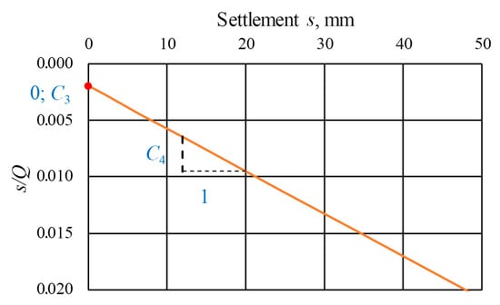 Figure 1. Graphical interpretation of the C3 and C4 constants.
From this equation, according to Chin (1970) [11], the limiting bearing capacity of the pile can be found, which is defined by the value to which the hyperbola asymptotically approaches
Both exponential shape functions (Method 1) and rectangular hyperbolas (Method 4) are highly suitable for describing phenomena where the variable asymptotically approaches a limiting value (asymptote). This would correspond to the graphs from static pile load tests when the s/D ratio is large and the end bearing capacity of the pile is low.
In Figure 2, all types of curves are presented, which are adapted to the results of the pile No 1 static load test.
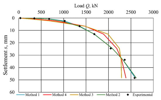
Figure 2.
Comparison of method and experimental test curves (Pile No 1).
In order to find out which of the curve types would be best suited to describe the behaviour of piles, a statistical analysis was performed based on the available static pile tests.
3. Analysis and Evaluation of Statistical Data
The field testing program was conducted between 2019 and 2025 at various active construction sites throughout Lithuania. All static load tests were performed by Geotechnikos grupė II Ltd in strict accordance with the requirements specified in the ISO 22477-1:2018 standards for geotechnical investigation and testing. The study involved the analysis of load–settlement curves (Appendix A) for 23 CFA-type piles. The specimen lengths ranged from 3 to 25 m, with diameters varying between 0.4 and 1.02 m. The piles were constructed using C25/30 grade concrete and reinforced with spatial cages fabricated from S500 class steel. Specific geometric properties, as well as the maximum applied test loads for each pile, are summarised in Table 1.

Table 1.
Experimental data of piles tested.
Vertical loads were applied to the pile head using one or more hydraulic jacks. Prior to the main testing sequence, a preliminary seating load ranging from 10 to 65 kN was applied to verify the functional integrity of the loading and measurement systems. The applied load was monitored via calibrated pressure gauges integrated into the hydraulic system, ensuring a measurement accuracy within 1% of the test load. The number of loading and unloading stages for each test is provided in Table 1.
Pile head displacements were recorded using a configuration of two or four VWDT-5004 vibrating wire displacement transducers Figure 3 (Geosense, UK), featuring a 50 mm stroke and a precision of ±0.1% of the full scale. The duration of each loading and unloading stage was governed by the observed displacement rates:
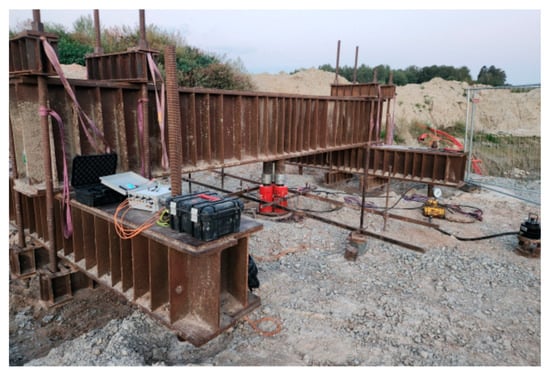
Figure 3.
Typical test setup featuring the settlement measurement system.
Loading stages: each increment was maintained for 30 min if the total pile head displacement was less than 1.5 mm, and for 60 min if the displacement exceeded this threshold.
Unloading stages: each decompression stage was held for 15 min if the elastic rebound was less than 1.5 mm, and for 30 min if the rebound exceeded 1.5 mm.
Final observation: upon reaching the fully unloaded state (0 kN), the pile status was monitored for a minimum duration of 60 min to ensure stabilisation.
Geological drilling and CPT tests were carried out near the tested piles. The soil stratigraphy is presented in Appendix B.
During pile tests, the ultimate bearing capacities of the piles were usually not reached. The maximum loads reached were related to the range of loads acting on the piles.
In the first stage of the study, the theoretical dependencies of the four aforementioned methods were recorded for the settlement load curves of pile tests using the least squares method. This was achieved using Excel function Solve (Figure 4).
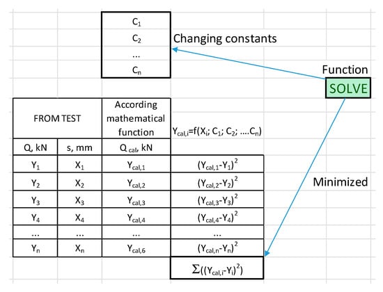
Figure 4.
Selection of constants of mathematical functions based on test results.
Following a preliminary analysis of the methods based on residual and scatter diagrams (see Appendix C), it was concluded that all methods were sufficiently accurate. The residual diagrams showed that the first two methods produced values that were closer together. Depending on the behaviour of the individual pile, the deviations of the theoretical load values from the experimental values are not in the same places on the graph according to the residual and scatter diagrams. Therefore, when choosing a method, attention must be paid to which part of the graph is important when using the method in further studies, e.g., when determining the bearing capacity of the pile base or evaluating the static model of the building.
However, only a deeper statistical analysis can objectively assess the accuracy of the methods.
Four evaluation criteria were adopted to determine accuracy: (1) Qtest/Qcalc correlation coefficients r of experimental and theoretical dependencies; (2) Qtest/Qcalc systematic and random errors; and (3) the coefficient of variation (4). Based on criteria 3–4, the analysed methods are also evaluated using the Demerit Point Method (DPC) [15] to assess their design safety.
Table 2 shows the summary of statistical results of the aforementioned evaluation criteria. All calculation data is presented in Appendix D. The calculations were performed and compared with the experimental values of 23 test piles. Each statistical criterion for each method and for each unique test was recalculated for eight experimental settlements, providing statistical results from a sufficiently large sample of 184 test points (23 × 8). The average calculated values of the statistical indicators are presented at the end of the table.
Table 2.
Summary of statistical evaluation criteria for the methods under consideration.
When analysing the correlation coefficient r presented in Table 2, it is particularly close to one for Methods 1 and 2. The average correlation coefficients for Methods 1 and 2 are 0.999 and 0.997, respectively. The correlation coefficient of the calculated values for Methods 1 and 2 is only 0.3%. This indicates very good agreement between the values. When analysing Methods 3 and 4, it can be seen that the correlation coefficients are slightly lower for different types of experimental soil. The lowest correlation value is 0.947 and the highest is 0.999. While the correlation coefficients do not differ significantly and all four Methods can be said to have a very strong correlation, the spread of the correlation coefficients calculated by Methods 3 and 4 around the mean is up to five times greater, amounting to 1.16%. In summary, while the correlation of all Methods is very strong, the most accurate are methods 1 and 2.
When analysing the second evaluation criterion, the systematic error μ∆R (average of Qtest/Qcalc), it can be seen that Methods 1 and 2 also have the highest accuracy. The systematic errors μ∆R of these Methods are 1.06 and 0.9, respectively, while those of Methods 3 and 4 are 1.60 and 1.41. It should be noted that the systematic errors μ∆R of Methods 3 and 4 are greater, particularly for small settlements. For example, of the 23 load–settlement dependencies calculated using Method 3, 5 values do not match the experimental results by a factor of between 2.46 and 3.23 (see Table 1 for details of samples No. 1, 2, 6, 18 and 23). The fourth method is more accurate. The results differ by more than three times only for sample No. 2. The values for samples 1, 6, 18 and 23 differ by less than 1.77–1.98. In summary, based on the systematic error criterion μ∆R, Methods 1 and 2 remain the most accurate.
For the comparison of systematic errors of the methods, an extended statistical analysis was additionally performed, using the correlation coefficients between the methods and the sensitivity of systematic errors with respect to soil type as evaluation criteria. Based on the calculation results presented in Appendix D, Table 3 shows the calculated correlation coefficients of Qtest/Qcalc for all four methods. As can be seen from the data, correlation relationships between the analysed methods are positive; however, their strength varies considerably, ranging from weak to strong. This indicates that the methods are neither completely independent nor can they be considered highly similar to each other. Method 1 exhibits weak correlation relationships with all other methods: a weak negative correlation is observed with Method 2 (r ≈ −0.11), indicating that these methods are essentially unrelated or even partially contradictory, while the relationships with Method 3 and Method 4 are only weakly positive (r ≈ 0.18 and r ≈ 0.27, respectively). Meanwhile, Method 2 shows moderate positive correlations with Method 3 (r ≈ 0.51) and Method 4 (r ≈ 0.39), suggesting that it is relatively close to these methods but not strongly associated with them. The strongest mutual relationship is identified between Method 3 and Method 4, for which the correlation is strong (r ≈ 0.78), indicating that these methods produce very similar results.
Table 3.
Correlation coefficients between the ratios of Qtest/Qcalc obtained using Methods 1–4.
After determination of the correlation relationships between the methods, the sensitivity of the systematic errors of the methods with respect to soil type was further analysed. The calculation results are presented in Table 4. The analysis of the results in Table 5 showed that Method 1 and Method 2 show the lowest sensitivity to soil properties compared to Method 3 and Method 4. The systematic error of Method 1 remains close to 1.0 in most soil types and increases only slightly in weak clays, indicating a limited dependence on soil type. Method 2 is characterised by the highest stability, with its error range in almost all cases varying between approximately 0.87 and 1.10, regardless of soil composition, density or degree of saturation. Due to these characteristics, Method 2 can be considered the most universal method.
Table 4.
Sensitivity of the systematic errors of the methods depending on soil type.
Table 5.
Ranking of methods according to the analysed statistical criteria.
When analysing the other methods, it was found that the smallest systematic errors of Method 3 and Method 4 occur in fine and silty medium-dense sands and in homogeneous medium-strength clays, where the errors are approximately 1.00–1.13 and 1.00–1.06, respectively. A moderate increase in error is observed in low-plasticity medium-strength clays and in sandy clays with gravel under non-saturated conditions, where the error range of Method 3 is approximately 1.25–1.40 and that of Method 4 is approximately 1.15–1.35. The largest errors are identified in dense and very dense sands, saturated silty or gravelly sands, and in weak clays containing gravel or organic inclusions. Under these conditions, the systematic error of Method 3 may reach up to 3.33, while that of Method 4 may reach up to 3.06. This demonstrates a strong dependence of the sensitivity of these methods on varying soil properties.
The same trends are observed when comparing the Methods according to the third and fourth criteria, i.e., the random error σ∆R of the average of Qtest/Qcalc values and the coefficient of variation in the random error. Methods 1 and 2 demonstrate the highest accuracy, with random σ∆R errors of 0.215 and 0.205, respectively. The random errors of Methods 3 and 4 are five times greater, making these methods significantly less accurate. When the analysis compared the coefficient of variation in the random error of the Qtest/Qcalc values, Method 1 is the most accurate. Its coefficient of variation is 0.18; the coefficients of variation in Methods 2, 4 and 3 are 0.222, 0.516 and 0.613, respectively.
It should be noted that systematic and random errors are both very important when calculating and evaluating the reliability of structures. In design standards such as EN 1990:2023 [16], these errors are included directly in the reliability calculation algorithm:
where
- μZ—mean value of safety margin function;
- σz—the standard deviation of the strength safety function Z; σxi—the standard deviation of the i-th term of the safety margin function, including the method’s random error σ∆R.
- μ∆R—systematic error of the method.
The reliability of the strength safety is calculated as the ratio between the mean value and the standard deviation of the strength safety distribution, expressed by the reliability index β. When calculating the strength safety function and its standard deviation, both the systematic method error μ∆R and the random method error σ∆R are included in the computations. Therefore, if the systematic method error is >1, the strength safety increases, and consequently, the reliability index β also increases. Conversely, an increase in the random method error leads to a higher standard deviation of the strength safety function, thereby decreasing the reliability index beta. Therefore, methods are considered more reliable when their systematic error is only slightly greater than 1 (since higher values would artificially increase reliability) and when their systematic error is minimal. Based on the data in Table 2, Methods 3 and 4 have very large random errors σ∆R (0.613 and 0.516), and are therefore less reliable than the first two methods. Although the random error of the second method is slightly smaller, its systematic error is <1 and equals 0.944. This indicates that Method 1 will be more reliable than Method 2, as its systematic error equals 1.06.
As mentioned earlier, the systematic errors can also be evaluated using the Demerit Point Method (DPC) [15]. According to this classification, when the systematic errors of the methods are inserted into the evaluation, Methods 1 and 2 fall into the “Appropriate and safe” group. Unfortunately, Methods 3 and 4 are classified as “Conservative methods.” Table 5 presents the ranking of the methods according to the criteria discussed above.
4. Conclusions and Suggestions
- Based on the residual and scatter diagrams, all four methods are suitable for mathematically describing the experimental pile load–settlement data. A more accurate evaluation of the methods can be obtained by applying statistical criteria, reliability indicators and the DPC method.
- After performing a statistical analysis of the load–settlement relationships of the four methods and comparing them with the experimental tests, and after summarising the results according to the four evaluation criteria (correlation coefficient, systematic and random method errors and coefficient of variation), it can be stated with statistical justification that the most accurate relationship is the quadratic hyperbolic curve (r = 0.9991; μ∆R = 1.06; σ∆R = 0.213, CoV = 0.181).
- The analysis of the systematic errors of the methods showed that the strongest positive correlation is observed between exponential shape and Method 4 (r ≈ 0.78). Power law exhibits moderate correlations with exponential shape and rectangular hyperbolas (r ≈ 0.39–0.51), whereas quadratic hyperbolic shows weak correlations with all other methods (|r| < 0.30). This indicating that quadratic hyperbolic is the most independent.
- The analysis of the sensitivity of the systematic errors with respect to soil type and soil properties showed that the lowest systematic errors for all methods occur in fine and silty medium-dense sands and in homogeneous medium-strength clays. The largest errors for exponential shape and rectangular hyperbolas were identified in dense and very dense sands, saturated sand–clay mixtures, weak low-plasticity clays, and fill materials, where the errors reach up to 3.33 and 3.06, respectively. Power law remains stable across all soil types, while quadratic hyperbolic exhibits only a weak dependence on soil properties. Therefore, from an engineering perspective, quadratic hyperbolic and power law are the most suitable methods.
- When the results are also evaluated using the DPC method, the “Appropriate and safe method” category likewise includes the quadratic hyperbolic curve and the power law distribution relationships.
- For practical calculations related to describing piles as supports, assessing their stiffness, the first two methods should be selected. Which of them is more suitable—based on the statistical methods described in this paper and the visual analysis of the residual diagrams—depends on the individual behaviour of each pile. This is because, according to the residual and scatter diagrams, the deviations of the theoretical load values from the experimental ones do not occur at the same points along the graph.
Author Contributions
Conceptualization, D.S., R.Š. and K.U.; methodology, D.S. and R.Š.; validation, D.S. and K.U.; formal analysis, R.Š.; investigation, R.Š. and K.U.; resources, D.S., R.Š. and K.U.; data curation, D.S., R.Š. and K.U.; writing—original draft preparation, D.S., R.Š. and K.U.; writing—review and editing, D.S., R.Š. and K.U.; visualization, D.S., K.U.; supervision, D.S.; project administration, K.U. All authors have read and agreed to the published version of the manuscript.
Funding
This research received no external funding.
Data Availability Statement
The original contributions presented in the study are included in the article.
Conflicts of Interest
The authors declare no conflicts of interest.
Appendix A. Pile Load Test (Pile No. 1–23)
Note: For clarity, the lower figure additionally shows piles with a settlement of up to 16 mm separately.


Appendix B. Soil Stratigraphy near Tested Piles
| Pile No | Soil Description | Layer Bottom Depth, m | qc, MPa | Pile Top Depth, m |
| 1 | Fill: sand | 0.9 | 8.0 | 0.9 |
| Silty sand; medium dense | 1.4 | 7.4 | ||
| Clay, medium plasticity, medium strength | 2.4 | 1.4 | ||
| Sandy silty clay; medium plasticity, medium strength | 3.6 | 1.9 | ||
| Sandy silty clay (till); low plasticity, stiff | 11.7 | 1.4…7.7 | ||
| 2 | Sand, gravelly sand; dense, very dense | 7.0 | 14.0…28.0 | 0.0 |
| 3 | Sand, gravelly sand; dense, very dense | 16.0 | 12.1…28.6 | 0.0 |
| 4 | Sand, gravelly sand; dense, very dense | 7.0 | 14.0…28.0 | 0.0 |
| 5 | Sand, gravelly sand; dense, very dense | 7.0 | 14.0…28.0 | 0.0 |
| 6 | Sand, gravelly sand; dense, very dense | 7.0 | 14.0…28.0 | 0.0 |
| 7 | Fine sand, silty sand; medium dense | 2.5 | 5.0…7.0 | 0.5 |
| Sandy low-plasticity clay (till), medium strength, with gravel | 13 | 1.2…2.4 | ||
| 8 | Fine sand, silty sand; medium dense | 2.5 | 5.0…7.0 | 0.5 |
| Sandy low-plasticity clay (till), medium strength, with gravel | 13 | 1.2…2.4 | ||
| 9 | Fine sand, silty sand; medium dense | 2.5 | 5.0…7.0 | 0.5 |
| Sandy low-plasticity clay (till), medium strength, with gravel | 13 | 1.2…2.4 | ||
| 10 | Sandy low-plasticity clay (till), light brown, weak, with gravel and pebbles up to 3–5%, from 1.9 m—medium strength, with lenses of saturated sand, from 6.0 m—grey, with heavy lenses of saturated sand, from 14.7 m—strong | 26.0 | 0.6…3.3 | 3.2 |
| 11 | Sandy low-plasticity clay (till), greyish brown, medium strength, with gravel and pebbles up to 3–5%, with lenses of wet sand, from 1.0 m—brown, from 1.5 m—with lenses of saturated sand, from 3.0 m—grey, from 18.0 m—strong, from 24.5 m—very strong | 33.0 | 2.0…6.9 | 2.8 |
| 12 | Sandy medium-plasticity clay, medium strength, with lenses of wet sand | 2.9 | 1.3 | 3.5 |
| Sandy low-plasticity clay (till), medium strength, with gravel and pebbles up to 3–5%, with lenses of wet sand, from 3.2 m—with lenses of saturated sand, from 10.4 m—strong, from 20.8 m—very strong | 29.0 | 2.2…6.4 | ||
| 13 | Sandy low-plasticity clay (till), weak, with gravel and pebbles up to 3–5%, from 2.0 m—medium strength, from 2.5 m—with lenses of saturated sand, in intervals 4.1–5.1 m and 9.6–11.0 m—weak, from 14.6 m—strong, from 24.5 m—medium strength | 25.7 | 0.8…3.8 | 3.9 |
| Clayey sand low-plasticity (till), very strong, with lenses of saturated sand | 28.0 | 20.2 | ||
| 14 | Sandy low-plasticity clay (till), medium strength, with gravel and pebbles up to 3–5%, from 2.4 m—strong, from 2.6 m—with lenses of saturated sand | 26.0 | 2.1…3.4 | 2.5 |
| 15 | Sandy low-plasticity clay (till), medium strength, with gravel and pebbles up to 3–5%, from 1.8 m—with lenses of saturated sand, in interval 3.0–3.6 m—weak | 8.4 | 0.9…1.5 | 1.5 |
| Sandy low-plasticity clay and silt (till), strong, with gravel and pebbles | 9.0 | 3.8 | ||
| Sandy low-plasticity silt, very strong, saturated, with lenses of silty sand | 12.0 | 9.7 | ||
| Sandy low-plasticity clay and silt (till), strong, with gravel and pebbles up to 3–5%, with lenses of saturated sand | 30 | 3.9…5.1 | ||
| 16 | Medium-plasticity clay, medium strength, from 2.0 m—with microlenses of saturated sand | 3.4 | 2.1 | 2.6 |
| Sandy low-plasticity clay (till), weak, with gravel and pebbles up to 3–5%, with lenses of saturated sand, from 5.2 m—medium strength, from 6.5 m—with heavy lenses of saturated sand, from 28.4 m—strong | 34.0 | 0.9…3.1 | ||
| 17 | Low-plasticity clay, weak, from 1.3 m—medium strength, with lenses of saturated sand, from 4.6 m—strong, silty | 6.9 | 1.0…2.9 | 2.9 |
| Silty sand, dense, saturated, clayey | 8.0 | 8.7 | ||
| Sandy low-plasticity clay (till), strong, with gravel and pebbles up to 3–5%, with lenses of saturated sand | 34.0 | 2.9…3.7 | ||
| 18 | Sandy low-plasticity clay weak, with organic | 4.9 | 0.5…0.9 | 0.2 |
| Sandy low-plasticity clay, medium strength | 21.0 | 1.2…2.2 | ||
| 19 | Sandy low-plasticity clay weak, with gravel and pebbles up to 3%, with lenses of saturated sand, from 1.4 m—medium strength | 5.1 | 0.6…1.4 | 3.8 |
| Sandy low-plasticity clay (till), strong, with gravel and pebbles up to 3–5%, with lenses of saturated sand, from 5.8 m—medium strength, from 7.0 m—with heavy lenses of saturated sand, from 13.3 m—strong | 14.5 | 1.8…4.4 | ||
| Sandy low-plasticity clay and silt (till), very strong, with gravel and pebbles up to 5–7%, with lenses of saturated sand | 18.6 | 7.3 | ||
| A little silty-clayey uniformly graded sand, very dense, saturated, with lenses of silty sand | 26.0 | 29.8 | ||
| 20 | Sandy low-plasticity clay, medium strength, from 1.1 m—weak, from 2.0 m—with microlenses of saturated sand | 3.3 | 0.4…1.5 | 2.1 |
| Sandy low-plasticity silt, strong, saturated | 3.8 | 2.2 | ||
| Sandy low-plasticity clay (till), medium strength, with gravel and pebbles up to 3–5%, with lenses of saturated sand, from 11.1 m—strong, in interval 12.7–13.4 m—very strong | 14.8 | 1.5…9.3 | ||
| A little silty-clayey uniformly graded sand, dense, saturated, with rare gravel | 16.0 | 19.6 | ||
| Sandy low-plasticity clay (till), medium strength, with gravel and pebbles up to 3–5%, with lenses of saturated sand, from 17.3 m—strong, from 18.1 m—very strong | 18.9 | 2.1…8.4 | ||
| A little silty-clayey uniformly graded sand, very dense, saturated, with rare gravel, in interval 21.0–22.5 m—dense | 26.0 | 15.8…25.7 | ||
| 21 | Medium-plasticity clay, with sand lenses | 2.3 | 1.4 | 3.6 |
| Silty sand | 3.2 | 8.3 | ||
| Medium-plasticity clay with sand lenses | 16.8 | 2.3…4.4 | ||
| Fine sand, dense | 20 | 36.5 | ||
| 22 | Low-plasticity clay, with sand | 4.4 | 0.9…3.4 | 3.7 |
| Fine sand | 6.0 | 3.6…15.8 | ||
| Low-plasticity clay | 8.8 | 3.8…5.3 | ||
| Silty sand, with clay lenses | 13.5 | 17.1…21.6 | ||
| Low-plasticity clay | 20.0 | 3.3…6.4 | ||
| 23 | File sand | 0.8 | 2.4 | 4.1 |
| Medium-plasticity clay | 1.8 | 1.3 | ||
| Sandy silt, medium-plasticity | 7.0 | 4.0…9.5 | ||
| Silty sand; dense | 20.0 | 12.0…20.0 |
Appendix C. Residual and Scatter Diagrams of Piles Tested (Pile No. 1–23)
Residual diagram
Method 1

Method 2

Method 3

Method 4

Scatter diagrams
Method 1

Method 2

Method 3

Method 4

Where Qcal is the calculated value, Qtest—the observed value (determined during the pile test).
Appendix D. Statistical Evaluation Criteria for the Methods Under Consideration
| Test. Nr. | Method 1 | Method 2 | Method 3 | Method 4 | ||||||||||||
| r | Avg | Stdev | CoV | r | Avg | Stdev | CoV | r | Avg | Stdev | CoV | r | Avg | Stdev | CoV | |
| 1 | 0.999702989 | 1.081031 | 0.238894 | 0.220988 | 0.997849 | 0.908935 | 0.260715 | 0.286836 | 0.969201 | 2.642193 | 3.127056 | 1.183508 | 0.980204 | 1.869065 | 1.76361 | 0.943579 |
| 2 | 0.999789173 | 1.093166 | 0.268128 | 0.245276 | 0.999237 | 1.127411 | 0.362589 | 0.321612 | 0.997277 | 3.327911 | 6.154284 | 1.849293 | 0.997824 | 3.057258 | 5.48539 | 1.794219 |
| 3 | 0.999813114 | 1.000467 | 0.010994 | 0.010989 | 0.99427 | 0.980299 | 0.098219 | 0.100192 | 0.996426 | 1.043053 | 0.109958 | 0.10542 | 0.999458 | 1.011806 | 0.039687 | 0.039224 |
| 4 | 0.996748526 | 0.981073 | 0.119177 | 0.121476 | 0.992538 | 0.978035 | 0.169019 | 0.172815 | 0.969739 | 1.113388 | 0.224462 | 0.201603 | 0.984869 | 1.03043 | 0.136165 | 0.132144 |
| 5 | 0.999878639 | 0.99974 | 0.015242 | 0.015246 | 0.998203 | 1.070294 | 0.2098 | 0.196021 | 0.992104 | 1.50168 | 1.22482 | 0.815633 | 0.992864 | 1.423143 | 1.060953 | 0.745499 |
| 6 | 0.999744997 | 1.000331 | 0.018281 | 0.018275 | 0.999694 | 1.014899 | 0.055308 | 0.054496 | 0.979461 | 2.55126 | 3.600834 | 1.411394 | 0.985658 | 1.985569 | 2.378984 | 1.198137 |
| 7 | 0.999923751 | 1.000366 | 0.008058 | 0.008055 | 0.997065 | 0.983441 | 0.073019 | 0.074249 | 0.991538 | 1.091988 | 0.220246 | 0.201692 | 0.997158 | 1.039109 | 0.113287 | 0.109023 |
| 8 | 0.999274311 | 0.999785 | 0.018813 | 0.018817 | 0.998361 | 0.99481 | 0.045987 | 0.046227 | 0.973258 | 1.130636 | 0.347244 | 0.307122 | 0.987168 | 1.056829 | 0.182744 | 0.172917 |
| 9 | 0.99948908 | 0.995484 | 0.0313 | 0.031442 | 0.998818 | 0.989872 | 0.057845 | 0.058436 | 0.998047 | 1.01695 | 0.046467 | 0.045692 | 0.998745 | 1.007906 | 0.031731 | 0.031482 |
| 10 | 0.999931695 | 0.97064 | 0.087133 | 0.089769 | 0.988942 | 0.873352 | 0.31651 | 0.362409 | 0.988386 | 1.255749 | 0.376635 | 0.299929 | 0.996782 | 1.096752 | 0.165041 | 0.150482 |
| 11 | 0.999575633 | 1.133825 | 0.343697 | 0.303131 | 0.999224 | 0.918365 | 0.195403 | 0.212773 | 0.994934 | 1.473204 | 0.942231 | 0.63958 | 0.997142 | 1.339854 | 0.720705 | 0.537898 |
| 12 | 0.999423468 | 1.239903 | 0.596967 | 0.481462 | 0.997891 | 0.917709 | 0.179988 | 0.196127 | 0.998024 | 1.419536 | 0.928771 | 0.654278 | 0.999085 | 1.322836 | 0.754619 | 0.570456 |
| 13 | 0.999580773 | 1.474278 | 1.270983 | 0.862105 | 0.996925 | 0.911496 | 0.190772 | 0.209296 | 0.99652 | 1.7267 | 1.799687 | 1.04227 | 0.998918 | 1.542634 | 1.417739 | 0.919038 |
| 14 | 0.999740921 | 1.070682 | 0.162301 | 0.151587 | 0.995785 | 0.885691 | 0.27725 | 0.313032 | 0.989507 | 1.395042 | 0.667718 | 0.478637 | 0.996086 | 1.214147 | 0.398318 | 0.328064 |
| 15 | 0.999227213 | 1.007169 | 0.051654 | 0.051286 | 0.991651 | 0.873542 | 0.314799 | 0.36037 | 0.987152 | 1.405242 | 0.644665 | 0.458757 | 0.995535 | 1.207085 | 0.354044 | 0.293305 |
| 16 | 0.998618978 | 1.077661 | 0.146716 | 0.136143 | 0.997566 | 0.89591 | 0.263491 | 0.294105 | 0.991557 | 1.271817 | 0.427965 | 0.336499 | 0.995975 | 1.148272 | 0.254454 | 0.221598 |
| 17 | 0.998165765 | 1.263936 | 0.595636 | 0.471255 | 0.999575 | 0.931991 | 0.163469 | 0.175398 | 0.99629 | 1.36978 | 0.774921 | 0.565726 | 0.96833 | 1.768428 | 1.407571 | 0.795945 |
| 18 | 0.999397141 | 0.996097 | 0.026708 | 0.026812 | 0.996147 | 0.98909 | 0.083361 | 0.08428 | 0.956426 | 2.464865 | 2.552551 | 1.035575 | 0.996144 | 1.012826 | 0.051177 | 0.050529 |
| 19 | 0.999470477 | 0.980746 | 0.067347 | 0.068669 | 0.997846 | 0.897985 | 0.264873 | 0.294964 | 0.991992 | 1.2279 | 0.329173 | 0.268078 | 0.96833 | 1.768428 | 1.407571 | 0.795945 |
| 20 | 0.99998256 | 0.999488 | 0.009326 | 0.009331 | 0.996874 | 0.89071 | 0.275463 | 0.309263 | 0.984139 | 1.641278 | 1.022788 | 0.623166 | 0.96833 | 1.768428 | 1.407571 | 0.795945 |
| 21 | 0.998813716 | 0.863481 | 0.377854 | 0.437593 | 0.996676 | 0.877638 | 0.320795 | 0.365521 | 0.9973 | 0.992277 | 0.32164 | 0.324143 | 0.998739 | 0.955369 | 0.296216 | 0.310054 |
| 22 | 0.994624372 | 1.087542 | 0.150304 | 0.138205 | 0.99719 | 0.906042 | 0.250607 | 0.276595 | 0.991316 | 1.169184 | 0.26224 | 0.224293 | 0.994535 | 1.089297 | 0.15522 | 0.142495 |
| 23 | 0.999120746 | 1.117471 | 0.27444 | 0.24559 | 0.99319 | 0.895062 | 0.301528 | 0.33688 | 0.946891 | 2.464865 | 2.552551 | 1.035575 | 0.96833 | 1.768428 | 1.407571 | 0.795945 |
| Avg | 0.999132089 | 1.062364 | 0.212607 | 0.181022 | 0.996588 | 0.944025 | 0.205687 | 0.221822 | 0.985978 | 1.5955 | 1.246039 | 0.613385 | 0.989835 | 1.412343 | 0.930016 | 0.516258 |
References
- Garcia, J.R.; de Albuquerque, P.J.R.; Santos, P.R.C.D.; de Freitas Neto, O. Analysis of the behavior of piled foundations in unconventional soil. Eng. Struct. 2024, 319, 118832. [Google Scholar] [CrossRef]
- Liu, H.; Xiao, Z.; Lee, K. Load-Settlement Behaviour Analysis Based on the Characteristics of the Vertical Loads under a Pile Group. Appl. Sci. 2022, 12, 6282. [Google Scholar] [CrossRef]
- Li, Q.; Wang, X.; Gavin, K.; Jiang, S.; Diao, H.; Wang, K. Influence of Scour Protection on the Vertical Bearing Behaviour of Monopiles in Sand. Water 2024, 16, 215. [Google Scholar] [CrossRef]
- Turskis, Z.; Urbonas, K.; Sližytė, D.; Medzvieckas, J.; Mackevičius, R.; Šapalas, V. A Novel Integrated Approach to Solve Industrial Ground Floor Design Problems. Sustainability 2020, 12, 4809. [Google Scholar] [CrossRef]
- ISO 22477-1:2018; Geotechnical Investigation and Testing—Testing of Geotechnical Structures—Part 1: Testing of Piles: Static Compression Load Testing. International Organization for Standardization (ISO): Geneva, Switzerland, 2018.
- Sližytė, D.; Šalna, R.; Urbonas, K. Statistical Evaluation of Sleeve Friction to Cone Resistance Ratio in Coarse-Grained Soils. Buildings 2024, 14, 745. [Google Scholar] [CrossRef]
- Nguyen, T.T.; Le, V.D.; Huynh, T.Q.; Nguyen, N.H.T. Influence of Settlement on Base Resistance of Long Piles in Soft Soil—Field and Machine Learning Assessments. Geotechnics 2024, 4, 447–469. [Google Scholar] [CrossRef]
- Bai, F.; Lu, Y.; Yang, J. Multi-Scale Investigation on Bearing Capacity and Load-Transfer Mechanism of Screw Pile Group via Model Tests and DEM Simulation. Buildings 2025, 15, 3581. [Google Scholar] [CrossRef]
- Kondner, R.L. Hyperbolic stress–strain response: Cohesive soils. J. Soil Mech. Found. Div. 1963, 89, 115–144. [Google Scholar] [CrossRef]
- Der Veen, V. The bearing capacity of a pile. In Proceedings of the Third International Conference on SMFE, Zurich, Switzerland, 16–27 August 1953; Volume 2, pp. 84–90. [Google Scholar]
- Chin, F.K. Estimation of the Ultimate Load of Piles from Tests Not Carried to Failure. In Proceedings of the Second Southeast Asian Conference on Soil Engineering, Singapore, 11–15 June 1970; pp. 81–92. [Google Scholar]
- Lastiasih, Y.; Irsyam, M.; Sidi, I.D. Reliability Study On Methods To Estimate Pile Load Capacity Based On Pile Loading Test Results in Indonesia. In Proceedings of the 18th Southeast Asian Geotechnical Conference (18SEAGC) Cum Inaugural Agssea Conference (1AGSSEA), Singapore, 29–31 May 2013. [Google Scholar] [CrossRef]
- Clauset, A.; Shalizi, C.R.; Newman, M.E.J. Power-Law Distributions in Empirical Data. SIAM Rev. 2009, 51, 661–703. [Google Scholar] [CrossRef]
- Wu, X.Z.; Xin, J.-X. Probabilistic analysis of site-specific load-displacement behaviour of cement-fly ash-gravel piles. Soils Found. 2019, 59, 1613–1630. [Google Scholar] [CrossRef]
- Collins, M.P. Evaluation of shear design procedures for reinforced concrete members under axial compression. ACI Struct. J. 2001, 98, 537–547. [Google Scholar] [CrossRef] [PubMed]
- EN 1990:2023; Eurocode—Basis of Structural and Geotechnical Design. European Committee for Standardization (CEN): Brussels, Belgium, 2023.


Disclaimer/Publisher’s Note: The statements, opinions and data contained in all publications are solely those of the individual author(s) and contributor(s) and not of MDPI and/or the editor(s). MDPI and/or the editor(s) disclaim responsibility for any injury to people or property resulting from any ideas, methods, instructions or products referred to in the content. |
© 2026 by the authors. Licensee MDPI, Basel, Switzerland. This article is an open access article distributed under the terms and conditions of the Creative Commons Attribution (CC BY) license.