Enhancing Seismic Displacement Prediction for Reinforced Concrete Box Girder Bridges Through Nonlinear Time History Analysis

Abstract

Inelastic displacement ratios are critical parameters in the seismic design of reinforced concrete (RC) box girder bridges. Existing approaches of displacement prediction, including the Displacement Coefficient Method and the Capacity Spectrum Method, typically rely on simplified single-degree-of-freedom (SDOF) models, which do not fully account for the complex and nonlinear behavior of multi-degree-of-freedom (MDOF) bridge systems. Moreover, the AASHTO Guide Specifications apply the equal displacement rule through the inelastic displacement modification factor R_d, which may underestimate displacement demands for short-period structures. This study evaluates the accuracy of the AASHTO R_d using nonlinear time history analyses of six RC box girder bridge models subjected to 28 recorded ground motions from California. Each ground motion included two orthogonal components applied in the longitudinal and transverse direction. Both elastic and inelastic displacement demands were determined in each direction, and inelastic displacement ratios (C_μ) were computed and compared with AASHTO predictions. A new predictive equation for C_μ was developed to capture response variability. While AASHTO R_d aligns with the average behavior, it fails to provide reliable estimate across the full range of seismic conditions. A comprehensive parametric study was conducted to examine the influence of column boundary condition, column height, superstructure deck width, number of spans, and damping ratio on C_μ. While the elastic and inelastic displacement decreases with an increase in damping ratio, the result shows that C_μ increases with higher damping ratios. Accordingly, a revised amplification factor was proposed to better represent the inelastic displacement demand in MDOF bridge systems.

1. Introduction

Bridges, as critical components of transportation infrastructure, require a resilient seismic design to ensure their functionality and safety following earthquakes. Since lateral displacement plays a direct role in structural damage, stability, and serviceability, modern seismic design philosophies have shifted toward performance-based design (PBD). This approach offers a more accurate assessment of structural performance under seismic loading compared to traditional strength-based methods, which primarily focus on force resistance without explicitly considering displacement demand [1]. Past earthquakes, such as the 1989 Loma Prieta and 1994 Northridge events, have highlighted the necessity of incorporating damage control mechanisms in structural design. The shift toward performance-based earthquake design underscores the importance of controlling structural displacement to minimize damage and enhance resilience [2]. Probabilistic seismic demand model, a critical component of performance-based earthquake engineering, is another approach to design the structures which considers the energy-related demands of ground motion [3,4].

The earthquake-induced inelastic displacement ratio is defined as the ratio of a structure’s maximum lateral inelastic displacement to its maximum lateral elastic displacement under seismic loading. While nonlinear time history analysis offers the most accurate estimation of inelastic response, its complexity and computational demands make it impractical for routine design applications. Consequently, simplified methods are required to estimate maximum inelastic displacement.

Over the past three decades, earthquake-resistant design philosophies have undergone significant evolution. Initially, strength-based design relied on response reduction factors to estimate structural strength by accounting for ductility, overstrength, and redundancy. However, this approach does not effectively control damage during moderate earthquakes, highlighting the increasing relevance of displacement-based design. Performance-based design (PBD) integrates both strength- and displacement-based principles [5,6,7], ensuring that structures meet predefined performance levels under varying earthquake intensities.

The lateral displacement or drift of the structures when subjected to earthquake ground motion causes both structural and nonstructural damage [8]. According to Section C.4.7.4.5 of AASHTO LRFD [9], earthquakes may cause instability issues in bridges due to $P-∆$ effects. The inadequate strength of bridges can result in ratcheting of structural displacements to larger values which causes an excessive ductility demand on plastic hinges in columns and possibly leads to its collapse. To prevent such effects on bridges, it is thus important to clearly understand the displacement behavior of bridges under earthquakes and accurately estimate the displacement demand so that the bridges can be adequately designed to sustain such $P-∆$ effects.

To facilitate the displacement estimation, various indirect methods have been developed. Rosenblueth and Herrera [10], Gulkan and Sozen [11], and Iwan [12], among others, introduced the concept of equivalent linear viscous damping and stiffness within an equivalent linearization technique. This method approximates the maximum displacement using an equivalent linear elastic system with reduced lateral stiffness and an increased damping coefficient compared to the inelastic system.

Two widely used methods for estimating maximum inelastic displacement demand are the displacement coefficient method and the capacity spectrum method. These approaches combine nonlinear static analysis with results from linear dynamic analysis to approximate inelastic displacement.

The capacity spectrum method, an iterative procedure used in the nonlinear static procedure (NSP), is implemented in ATC-40 [13] and is based on the equivalent linearization technique developed by earlier researchers [10,11,12]. Originally developed for seismic risk assessment at the Puget Sound Naval Shipyard for the U.S. Navy in the early 1970s [14], this method has undergone various refinements while maintaining its fundamental principles. ATC-40 estimates maximum inelastic displacement through an iterative analysis of equivalent linear elastic systems, characterized by an equivalent viscous damping ratio and secant stiffness, both of which are dependent on inelastic deformation.

The displacement coefficient method operates under the premise that the inelastic displacement of a yielding structure can be estimated by multiplying the spectral displacement of a linear elastic single-degree-of-freedom (SDOF) system with a displacement modification factor. This factor, known as the inelastic displacement ratio, has been proposed by several researchers, including Newmark and his colleagues [2,8,15,16,17,18,19,20]. Design guidelines such as FEMA 273 [21], FEMA 356 [22], and FEMA 440 [23] have also adopted this method to estimate displacement demand within the nonlinear static procedure (NSP) framework. Early studies on the displacement coefficient method were conducted by Veletsos and Newmark [24] and Veletsos et al. [25], who observed that for flexible oscillators, the ratio of maximum deformation in a nonlinear system to that in a linear system is unity, leading to the equal displacement rule. However, for stiff oscillators, this ratio exceeds unity. Veletsos and Vann [26] later extended the applicability of this rule to medium-frequency oscillators, while Newmark and Hall [16] and Riddell [27] identified a period threshold above which the equal displacement rule remains valid.

Miranda [8] conducted a study on 124 earthquake ground motions across various site conditions and concluded that the inelastic displacement ratio depends on factors such as period, ductility demand, and site conditions. Further research by Miranda [17] demonstrated that soil conditions have minimal influence on inelastic displacement ratios when shear-wave velocities exceed 180 m/s. Later, Ruiz-Gracia and Miranada [28] performed a detailed study on constant relative strength inelastic displacement ratio in SDOF system considering three different types of soil conditions.

Hatzigeorgiou and Beskos [29] proposed a method for estimating the inelastic displacement ratio for a bilinear elastoplastic SDOF system subjected to multiple earthquakes. Their equation incorporated the effects of damping ratio, post-yield stiffness ratio, and soil type, emphasizing that repeated earthquakes significantly influence inelastic displacement ratios. Wu et al. [30] formulated an equation for inelastic displacement demand specific to Chinese highway bridges, modeled as bilinear SDOF systems. Similarly, Bozorgnia et al. [31] conducted deterministic and probabilistic predictions of inelastic response spectra, revealing that inelastic system scaling magnitude exceed those of elastic systems, particularly for large earthquakes.

Most studies on inelastic displacement ratio have focused on SDOF systems with elastic-perfectly plastic or bilinear elastoplastic models. However, real structures, such as bridges, are MDOF systems that exhibit nonlinear behavior at various structural components. Zhang et al. [5] studied shear-flexure interaction in bridge columns subjected to multidirectional shaking by modeling 24 full-scale columns. While they developed a model to estimate inelastic displacement and ductility, their study did not consider nonlinear abutment behavior, highlighting the need for further research on complete bridge systems to enhance accuracy in estimating inelastic displacement ratio.

Current design methodologies rely on the equal displacement rule for long periods, with ductility-dependent magnification factors applied at short periods. The AASHTO Seismic Bridge Design Guide [32] and AASHTO LRFD [9], estimate inelastic demands using an elastic analysis approach based on the equal displacement approximation when the fundamental period exceeds the characteristic ground motion period (T*). For short-period structures (T < T*), AASHTO recommends multiplying the elastic displacement demand (${∆}_D$) by magnification factor $R_d$. AASHTO guidelines assume a 5% viscous damping ratio, with a reduction factor $R_D={\left({\displaystyle \frac{0.05}{\zeta }}\right)}^{0.4}$ applied for other damping values.

Martinez and Kowalsky [33] outlined that AASHTO Seismic Bridge Design Guide [32] significantly underpredicts the displacement demand as compared to Nonlinear time history analysis. The possible underestimation with AASHTO equation has also been verified by NCHRP completed project NCHRP 12-106 [34]. Furthermore, few studies have focused on modeling entire bridge structures with their nonlinear behaviors, leaving a significant gap in current research. To address these limitations, this study evaluates the reliability of AASHTO $R_d$ using recorded earthquake data and aims to develop a more accurate method for estimating inelastic displacement ratios in box girder bridges. By considering various bridge geometries and seismic events, this research proposes an improved approach to enhance the accuracy of seismic design methodology, ensuring better prediction of bridge performance under earthquake loading. In this paper, the literature review and background on the inelastic displacement demand research of bridges under earthquake is summarized in Section 1. The modeling methodology of bridges under earthquakes through a MDOF system is included in Section 2. Results and discussions are analyzed in Section 3 with a parametric study of deck width, number of spans, column height, column to ground connection, and damping ratio. In Section 4, conclusions and recommendations of the study are summarized for potential implementations.

2. Methods

CSiBridge was used to model the earthquake responses of the bridges, incorporating both material and geometric nonlinearities through direct integration. The built model accounts for P-∆ effects as the guideline [35] suggests that P-∆ option is enough for typical bridges, especially when the material nonlinearity dominates the nonlinear behavior. Uncertainty in numerical simulations always exists, which may slightly affect the conclusion reached.

The analysis uses six of California’s seismically active reinforced concrete box-girder bridges: two Ordinary Standard Bridges (OSB1 and OSB2) from Caltrans, along with Route 14 Left (R14L), Route 14 Right (R14R), La Veta, and Adobe bridges. Both pinned and fixed column-ground connections were considered, resulting in 12 bridge models for analysis. Three-dimensional models were developed using Caltrans as-built drawings and CSiBridge input files for OSB1 and OSB2 bridge models, with modifications such as a simplified abutment model based on the guideline [35] and adjusted rigid offset lengths in the columns. The detailed modeling techniques for bridges are based on the procedures explained in the reports [35,36,37,38] and each of the six bridges are explained in detail in the thesis report [39].

The study analyzed reinforced concrete box-girder bridges with varying spans, bent configurations, and structural details. Each bridge consists of single or multiple spans, with integral bent caps supported by circular columns of different diameters and reinforcements. Column heights were based on referenced studies or drawings, with geometry and material properties summarized in Table 1. Box-girder deck vary in width and depth, with rigid column-to-bent cap and column-to-deck connections. Initial models were validated against existing study [37], with refinements in girder modeling, abutment representation, and rigid offsets. Three-dimensional models include the superstructure deck, bent cap, columns, and abutments, with abutments modeled as massless rigid elements constrained in all degrees of freedom. Nonlinear longitudinal behavior in the abutment was represented by gap and multilinear plastic link elements.

Table 1. Geometry, material strength, and plastic hinge length of six bridges.

Geometry and Material Strength	Unit	Bridge Name
		R14_L	R14_R	Adobe	La Veta	OSB1	OSB2
Deck section
Total length	ft	285.43	285.43	203.08	299.87	300.00	300.00
Number of spans	-	2.00	2.00	2.00	2.00	2.00	2.00
Span 1	ft	144.36	144.36	102.79	154.86	150.00	150.00
Span 2	ft	141.08	141.08	100.30	145.01	150.00	150.00
Total deck width	ft	53.71	41.90	41.51	75.49	47.50	37.50
Deck depth	ft	5.74	5.74	4.10	6.23	6.00	6.00
Concrete material	ksi	4.00	4.00	4.00	4.00	3.60	4.00
Young’s modulus	ksi	3605.00	3605.00	3605.00	3605.00	3420.00	3605.00
Cap Beam
Cap beam width	ft	7.55	7.55	7.00	7.55	8.67	8.67
Cap beam depth	ft	5.74	5.74	4.10	6.23	6.00	6.00
Cap beam length	ft	43.32	31.64	35.49	64.99	41.50	31.50
Column
Number of columns	-	2.00	1.00	2.00	2.00	2.00	1.00
Location of column 1	ft	10.51	15.82	11.83	21.66	8.75	15.75
Location of column 2	ft	32.82		23.66	43.33	32.75
Height of column	ft	37.97	37.97	26.60	25.40	20.00	20.00
Diameter	ft	5.41	5.41	4.00	5.58	5.50	5.50
Plastic hinge
Length	ft	4.31	4.31	3.08	3.09	2.80	2.80

The column modeling approach proposed by Caltrans and discussed in the work Lu et al. [38] has been adopted in the present work. Column modeling includes discretized columns with plastic hinge locations and considers pinned or fixed boundary condition at the base to consider the envelope response of the foundation. Plastic hinge lengths, summarized in Table 1, were calculated based on Section 7.6.2 of Caltrans Seismic Design Criteria [40], which was also explained in the literature [41].

Nonlinear analysis incorporates abutment gap elements and multilinear plastic links with specific stiffness values. Simplified abutment model per guideline [35] was used to model the nonlinear behavior of abutment where a rigid element of length equal to the superstructure width, $d_w,$ is connected to the superstructure centerline through a rigid joint as shown in Figure 1. At both ends of the rigid element, the longitudinal, transverse, and vertical responses of the abutment were modeled using the link elements as shown in Figure 1, Figure 2 and Figure 3. Studies [35,37,38,40,42] were referred to for the detailed modeling approach and calculation of longitudinal, transverse and vertical stiffness of each link elements are explained in detail in thesis report [39]. The stiffness of those elements in each of the directions are summarized in Table 2 and Table 3. This standardized approach ensures consistency while maintaining bridge-specific characteristics, with typical visual models as shown in Figure 2 and Figure 3.

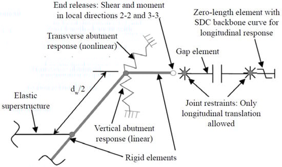
Figure 1. Simplified abutment model scheme representing rigid element of length equal to superstructure width being connected to the superstructure deck at the middle and to vertical spring, transverse spring and longitudinal series of elements at each end. The vertical spring represents the linear response of bearing pads; transverse spring represents the nonlinear response of backfill, wing wall, and pile system response; the series of elements in longitudinal direction consist of a rigid element, a gap element, and a zero-length element to represent the longitudinal response of the abutment [35].

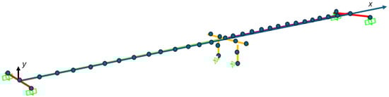
Figure 2. Three-dimensional spine model of a two-span OSB1 bridge created in CSiBridge, with the two-column single bent at the center of the bridge and simplified abutment model at the end of each span. The column has pinned boundary conditions with plastic hinge assigned at the top of the column that connects to the bent. The rigid element of length equal to deck width is modeled at the end of each span which connects to series of link element at each end. The blue and the purple color stand for two different spans of the bridge. The red color segments at the two ends indicate the bridge abutments with the dark green boxes for the supports., while the middle brown color segments are for bent columns. The dark blue circles are the CSiBridge model nodes, and the green boxes stand for the boundary conditions with ground.

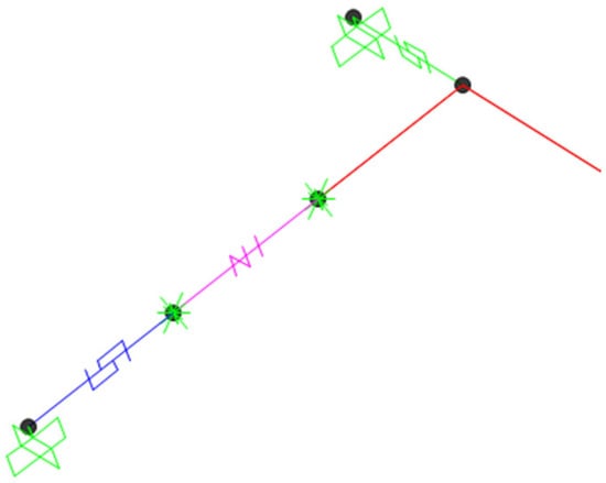
Figure 3. Simplified abutment model created in CSiBridge for OSB1 bridge using a multilinear plastic link element (green color) in transverse direction; a series of rigid element (red color), a gap element (magenta color), and a multilinear plastic link element (purple color) in longitudinal direction. The green color link element was used to define nonlinear properties in transverse direction and elastic stiffness in vertical direction. The magenta color gap element and purple color link element were used to define nonlinear property in longitudinal direction where both ends of gap element were restrained in transverse and vertical direction and all rotational degrees of freedom to allow the translation only in longitudinal direction.

Table 2. Bridge dimensions and longitudinal stiffness parameters for six bridges.

Bridge Dimension					Longitudinal Stiffness
Bridge	${\mathit{d}}_{\mathit{w}}$ (ft)	${\mathit{h}}_{\mathit{a}\mathit{b}\mathit{u}\mathit{t}}$ (ft)	${\mathit{w}}_{\mathit{a}\mathit{b}\mathit{u}\mathit{t}}$ (ft)	${\mathit{w}}_{\mathit{w}\mathit{w}}$(ft)	${\mathit{K}}_{\mathit{a}\mathit{b}\mathit{u}\mathit{t}}$ (kip/in)	${\mathit{F}}_{\mathit{a}\mathit{b}\mathit{u}\mathit{t}}$ (kip)	${∆}_{\mathit{g}\mathit{a}\mathit{p}}$ (in)	${∆}_{\mathit{a}\mathit{b}\mathit{u}\mathit{t}}$ (in)	${∆}_{\mathit{e}\mathit{f}\mathit{f}}$ (in)	${\mathit{K}}_{\mathit{e}\mathit{f}\mathit{f}}$ (kip/in)	$\frac{{\mathit{F}}_{\mathit{a}\mathit{b}\mathit{u}\mathit{t}}}{2}$ (kip)	$\frac{{\mathit{K}}_{\mathit{a}\mathit{b}\mathit{u}\mathit{t}}}{2}$ (kip/in)
R14L	53.7	5.7	42.2	17.9	2177.9	1255.8	2.0	0.58	2.58	487.4	627.9	1088.9
R14R	41.9	5.7	30.4	14.0	1568.7	904.5	2.0	0.58	2.58	351.1	452.3	784.3
Adobe	41.5	4.1	33.3	13.8	1417.2	581.8	2.0	0.41	2.41	241.4	290.9	708.6
La Veta	75.5	6.2	63.0	25.2	3421.3	2132.0	2.0	0.62	2.62	812.8	1066.0	1710.7
OSB1	47.5	6.0	35.5	15.8	1881.5	1131.2	2.0	0.60	2.60	434.9	565.6	940.8
OSB2	37.6	6.0	25.6	12.5	1356.8	815.8	2.0	0.60	2.60	313.6	407.9	678.4

Table 3. Transverse and vertical stiffness parameters for six bridges.

Transverse Stiffness						Vertical Stiffness
Bridge	${\mathit{K}}_{\mathit{a}\mathit{b}\mathit{u}\mathit{t}}$ (kip/in)	${\mathit{F}}_{\mathit{a}\mathit{b}\mathit{u}\mathit{t}}$ (kip)	${∆}_{\mathit{e}\mathit{f}\mathit{f}}$ (in)	$\frac{{\mathit{F}}_{\mathit{a}\mathit{b}\mathit{u}\mathit{t}}}{2}$ (kip)	$\frac{{\mathit{K}}_{\mathit{a}\mathit{b}\mathit{u}\mathit{t}}}{2}$ (kip/in)	${\mathit{K}}_{\mathit{v}}$ (kip/in)
R14L	820.78	473.27	0.58	236.64	410.39	481.19
R14R	640.28	369.19	0.58	184.60	320.14	481.19
Adobe	523.28	214.83	0.41	107.41	261.64	415.80
La Veta	1214.24	756.67	0.62	378.33	607.12	755.91
OSB1	745.93	448.48	0.60	224.24	372.96	720.00
OSB2	590.46	355.01	0.60	177.50	295.23	720.00

Where

$d_w$ = width of superstructure (ft)

$h_{abut}$ = height of backwall or diaphragm (ft)

$w_{abut}$ = width of abutment (ft)

$w_{ww}$ = width of wing wall (ft)

$K_{abut}$ = stiffness of abutment (kip/in)

$F_{abut}$ = idealized ultimate passive capacity of the abutment backfill (kip)

${∆}_{gap}$ = width of expansion gap in seat abutment (in)

${∆}_{abut}$ = abutment displacement at yield (in)

${∆}_{eff}$ = effective abutment longitudinal displacement (in)

$K_{eff}$ = effective abutment stiffness (kip/in)

$K_v$ = vertical elastic stiffness (kip/in)

This study examines earthquake ground motions affecting California bridges, selecting seismic events from 1970 to 2024 to match a typical bridge design lifespan of 50–70 years. The USGS Disaggregation Hazard Tool identified a mean earthquake magnitude of 6.23 and a closest rupture distance of 23.95 km at 36.374° latitude, −119.27° longitude, with a site-class BC (V_s30 = 760 m/s) and a 2% probability of exceedance in 50 years (return period: 2475 years). Ground motion records were sourced from the Pacific Earthquake Engineering Research Center (PEER) Ground Motion Database, selecting 28 earthquake motions for Nonlinear Time History Analysis (THA) of six bridges under two boundary conditions. Each earthquake includes three components (two horizontal, one vertical), though only horizontal motions were considered due to their dominant influence on bridge response. Key parameters such as magnitude, duration, Arias intensity, rupture distances, and $V_{s30}$ (timed-average shear-wave velocity to a depth of 30 m) are detailed in Appendix A Table A1. The two horizontal components of the earthquake ground motion as obtained from the PEER database were applied in U1 (longitudinal) and U2 (transverse) direction of the bridge.

A numerical model of six bridges, each with two column boundary conditions, was developed for seismic analysis. The response was evaluated using 28 earthquake ground motions per bridge, assuming a 5% baseline damping ratio. To assess damping effects, additional analyses were performed with 1%, 3%, and 7% damping. An extra span was added to all bridge models to examine its influence on the inelastic displacement ratio.

3. Results and Discussions

To validate the numerical modeling approach used in CSiBridge, a single-degree-of-freedom (SDOF) elastoplastic system was analyzed under the El Centro ground motion. This validation was benchmarked against the results provided by Chopra [43], who presented curves of peak inelastic displacement ($u_m$) versus peak elastic displacement ($u_e$) for various normalized yield strengths $\overline{f_y}$, defined as:

$$\overline{f_y}={\displaystyle \frac{f_y}{f_o}}={\displaystyle \frac{u_y}{u_o}}={\displaystyle \frac{u_y}{u_e}}$$

(1)

where $f_o$ and $u_o$ are the peak resisting force and deformation of a linear elastic system under earthquake excitation, respectively, and $f_y$ and $u_y$ are the yield force and displacement of the corresponding elastoplastic system. In CSiBridge, an SDOF model was constructed using a multilinear elastic link element with a lumped mass of 300 kips. The peak elastic displacements $u_e$ were computed for periods T = 0.125, 0.5, and 3 s. Corresponding yield displacements $u_y$ were derived for different values of $\overline{f_y}$. A nonlinear time history analysis was then performed to compute the peak inelastic displacements $u_m$, and the ratio was compared to Chopra’s benchmark curves. As shown in Figure 4, the results from CSiBridge (marked with symbols) closely follow Chopra’s analytical curves for all three values of $\overline{f_y}$ = 0.125, 0.25, and 0.5. The consistency across a wide range of periods validates the accuracy of the numerical model and confirms that the nonlinear time history analysis in CSiBridge reliably captures inelastic deformation behavior. Figure 4 presents the variation in normalized peak inelastic displacement $u_m$/$u_e$ with respect to the fundamental time period for three different normalized yield strengths. The solid blue, dotted red, and dashed black lines represent Chopra’s analytical results. The corresponding CSiBridge simulation results are shown as diamond, triangle, and circle markers. The close agreement between the analytical and numerical data points across the spectrum demonstrates that the modeling approach in CSiBridge is reliable for simulating nonlinear seismic behavior of SDOF systems.

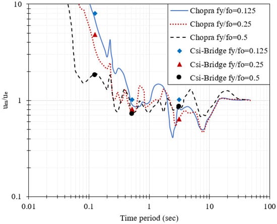
Figure 4. Validation of inelastic displacement ratios for SDOF system under El Centro Ground Motion—comparison between CSiBridge and Chopra [43].

The OSB1 bridge model, developed by Caltrans, was analyzed under CLAYN1N1 and SANDN1N1 earthquake ground motions [37]. The P-component of these ground motions, i.e., CLAYN1N1P and SANDN1N1P were applied along the longitudinal U1 direction in bridge model while N-component of these ground motions, i.e., CLAYN1N1N and SANDN1N1N were applied along the transverse U2 direction. The time period of the first six modes and inelastic displacements at the center of mass were compared with Mackie et al. [37], demonstrating strong agreement with the literature, as shown in Table 4 and Table 5. This validates the CSiBridge model of the OSB1 bridge in this study and confirms the accuracy of the model for nonlinear time history analysis. For the subsequent analyses, the ground motions listed in Table A1 were used and all other bridge models were developed based on the validated OSB1 bridge model using the corresponding geometric properties and nonlinear behavior of column and abutment of the respective bridge types, similar to Mackie et al. [37].

Table 4. Comparison of time period of first six modes of OSB1 bridge with literature.

Mode	Time Period (s)
	Mackie et al. [37]	Analysis
1	0.614	0.61054
2	0.609	0.60831
3	0.403	0.40246
4	0.352	0.35204
5	0.283	0.28312
6	0.157	0.15732

Table 5. Comparison of inelastic displacement of center of mass of OSB1 bridge with literature.

Description	Displacement (in.)
Earthquake Name	CLAYN1N1		SANDN1N1
	U1 (P-090)	U2 (N-000)	U1 (P-090)	U2 (N-000)
Analysis	5.796	4.941	3.234	5.530
Mackie et al. [37]		4.850	2.800	5.410

The inelastic displacement ratio has been defined as displacement magnification factor, $R_d,$ in Section 4.3.3 of AASHTO Seismic Bridge Design Guide [29] and Section 4.7.4.5 of AASHTO LRFD [9] and expressed as

$$R_d=\left(1-{\displaystyle \frac{1}{{\mu }_D}}\right){\displaystyle \frac{T^{*}}{T}}+{\displaystyle \frac{1}{{\mu }_D}}\ge 1.0 for {\displaystyle \frac{T^{*}}{T}}>1.0$$

(2)

$$R_d=1.0 for{\displaystyle \frac{T^{*}}{T}}\le 1.0$$

(3)

in which

$$T^{*}=1.25T_s=1.25{\displaystyle \frac{S_{D1}}{S_{DS}}}$$

(4)

where ${\mu }_D$ = maximum local member displacement ductility demand. For Seismic design category D, ${\mu }_D$ can be taken as 6 instead of a detailed analysis; $S_{D1}$ = 1 s period acceleration coefficient and can be obtained from the design response spectrum; $S_{DS}=$ the short-period acceleration coefficient and can be obtained from the design response spectrum

Considering the upper bound value of $T^{*}$, $T^{*}=1.25$ [44], $R_d$ can be expressed as

$$R_d=0.167+{\displaystyle \frac{1.042}{T}}$$

(5)

In this study, a similar general form, Equation (6), was adopted to ensure consistency with the AASHTO Equation (5).

$$C_{\mu }=0.167+{\displaystyle \frac{a}{T}}$$

(6)

The coefficient a was obtained using the MATLAB’s Curve Fitter application (MATLAB 2020b). Since the analyzed two-span bridge models exhibited fundamental periods between 0.35 and 0.55 s, three span bridge models were developed for all bridges and additional two span bridge models were developed by changing the length of superstructure deck to obtain the inelastic displacement ratio for the time period outside this range. Finally, the results of bridges with first mode of time period between 0.2 s and 1.0 s were obtained and plotted in Figure 5. The Mean, Mean plus Standard Deviation (Mean + SD), Mean plus three times Standard deviation (Mean + 3SD) and Root Mean Square Error (RMSE) of inelastic displacement ratios for all 28 earthquake ground motions in both longitudinal and transverse direction were calculated at each time period and listed in Table A2. RMSE values show that the data are distributed about the Mean value which can also be observed in Figure 5.

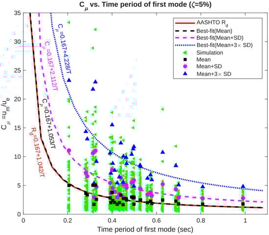
Figure 5. Inelastic displacement ratio vs. fundamental period of bridges for a damping ratio of 5%. Green triangles represent the inelastic displacement ratio for all 28 earthquake ground motions in longitudinal and transverse direction at each time period, while black squares, magenta circles and blue triangles represent the Mean, Mean + SD and Mean + 3 SD of those responses at each respective time period. The red solid line represents AASHTO $R_d$ equation, and black dash line represent the best fit equation obtained based on Mean values of inelastic displacement ratios for different time periods. It can be observed that the Mean values are in close agreement with AASHTO $R_d$. The magenta dash line and blue dash line represent the best-fit line based on Mean + SD and Mean + 3 SD to consider the response due to wide range of earthquake ground motion.

The best-fit equation ($C_{\mu }$) was obtained using the mean values and expressed in Equation (7) with R-squared ($R^2)=0.421$. The general equation for $C_{\mu }$ was constrained to follow the AASHTO form rather than being derived from a purely data-driven best-fit model. Consequently, the resulting R-squared values were low. Moreover, the fitted $C_{\mu }$ intends to provide a reliable level of inelastic displacement demand for different bridges and earthquakes. There is no physical meaning to link all the data points.

$$\mathbf{Mean}\mathbf{:} C_{\mu }=0.167+{\displaystyle \frac{1.053}{T}} ; R^2=0.421$$

(7)

This closely aligns with the original AASHTO $R_d$, indicating that AASHTO provides a reasonable estimate for the average inelastic displacement ratio across various ground motions. However, it is evident from Figure 4 that the AASHTO curve tends to underpredict $C_{\mu }$ for significant number of individual earthquake records. To account for this variability, two additional equations were developed by fitting Mean + SD values and Mean + 3SD values, expressed by Equation (8) and Equation (9), respectively.

$$\mathbf{Mean} \mathbf{+} \mathbf{SD}: C_{\mu }=0.167+{\displaystyle \frac{2.112}{T}} ; R^2=0.473$$

(8)

$$\mathbf{Mean} \mathbf{+} \mathbf{3}\mathbf{SD}: C_{\mu }=0.167+{\displaystyle \frac{4.228}{T}} ; R^2=0.476$$

(9)

Equations (8) and (9) provide more conservative estimates, which are particularly relevant for bridges located in seismically active regions such as California. As illustrated in Figure 4, although the AASHTO and mean equations capture the central tendency of the data, the Mean + SD and Mean + 3SD formulations encompass approximately 68% and 99.7% of the data, respectively, assuming a normal distribution. The Mean + SD equation can therefore be considered suitable for accounting for moderate variability in design, while the Mean + 3SD equation is more appropriate for capturing extreme cases, offering an upper-bound envelope for inelastic displacement demand.

The effect of column boundary conditions on the inelastic displacement ratio was investigated by reanalyzing bridge models. Separate fitted equations were derived for bridges with pinned and fixed column connections:

Pinned Connection:

$$\mathrm{Mean}: C_{\mu }=0.167+{\displaystyle \frac{1.353}{T}} ; R^2=0.820$$

(10)

$$\mathbf{Mean} \mathbf{+} \mathbf{SD}\mathbf{:} C_{\mu }=0.167+{\displaystyle \frac{2.715}{T}} ; R^2=0.740$$

(11)

Fixed Connection:

$$\mathrm{Mean}: C_{\mu }=0.167+{\displaystyle \frac{0.880}{T}} ; R^2=0.679$$

(12)

$$\mathbf{Mean} \mathbf{+} \mathbf{SD}\mathbf{:} C_{\mu }=0.167+{\displaystyle \frac{1.764}{T}} ; R^2=0.669$$

(13)

Comparing Equations (10) and (12), the result indicates that bridges with pinned column connections tend to exhibit higher inelastic displacement ratios compared to those with fixed connections. This difference is primarily attributed to the increased flexibility associated with pinned supports, which leads to greater displacement demands under seismic loading. While the AASHTO equation provides a conservative estimate for fixed columns, it underpredicts the inelastic displacement ratio for pinned configurations.

The effect of column height on the inelastic displacement ratio was investigated by categorizing bridge models into two height ranges: 20–30 ft and 30–40 ft. The corresponding fitted equations using Mean and Mean + SD for each group are given by Equations (14) and (15) and Equations (16) and (17), respectively.

20–30 ft:

$$\mathrm{Mean}: C_{\mu }=0.167+{\displaystyle \frac{0.990}{T}} ; R^2=0.166$$

(14)

$$\mathbf{Mean} \mathbf{+} \mathbf{SD}\mathbf{:} C_{\mu }=0.167+{\displaystyle \frac{1.923}{T}}; R^2=0.264$$

(15)

30–40 ft:

$$\mathrm{Mean}: C_{\mu }=0.167+{\displaystyle \frac{1.156}{T}} ; { R}^2=0.720$$

(16)

$$\mathbf{Mean} \mathbf{+} \mathbf{SD}\mathbf{:} C_{\mu }=0.167+{\displaystyle \frac{2.416}{T}}; R^2=0.763$$

(17)

As shown in Figure 6, bridges with taller columns (30–40 ft) exhibit higher inelastic displacement ratios compared to those with shorter columns (20–30 ft). The increased demand is reflected in both the simulation data and the best-fit trend lines. This behavior is primarily attributed to the reduced lateral stiffness of taller columns. Consequently, greater flexibility in taller columns leads to amplified inelastic displacements under seismic loading.

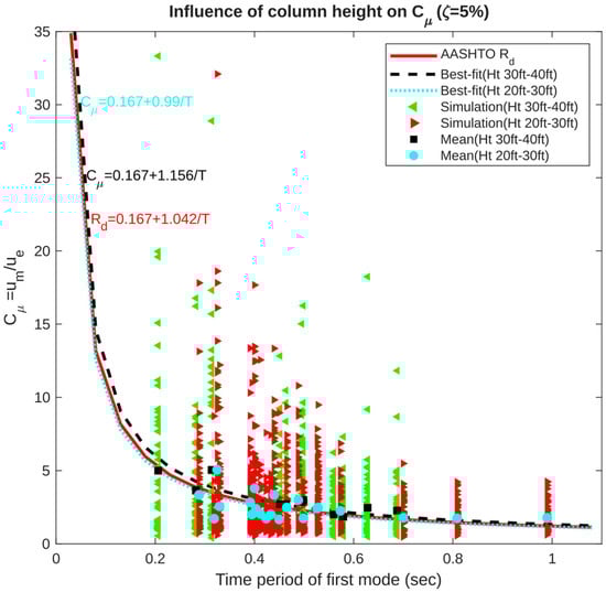
Figure 6. Influence of column height on inelastic displacement ratio for a damping ratio of 5% representing the inelastic displacement ratio increase with the increase in height of the column.

The effect of superstructure deck width on the inelastic displacement ratio was analyzed by categorizing the bridge models into two groups: 30–50 ft and 50–80 ft. The fitting equations for each group are as follows:

30–50 ft:

$$\mathbf{Mean}: C_{\mu }=0.167+{\displaystyle \frac{1.017}{T}} ; R^2=0.178$$

(18)

$$\mathbf{Mean} \mathbf{+} \mathbf{SD}: C_{\mu }=0.167+{\displaystyle \frac{1.989}{T}}; R^2=0.256$$

(19)

50–80 ft:

$$\mathbf{Mean}: C_{\mu }=0.167+{\displaystyle \frac{1.093}{T}}; R^2=0.545$$

(20)

$$\mathbf{Mean} \mathbf{+} \mathbf{SD}: C_{\mu }=0.167+{\displaystyle \frac{2.242}{T}}; R^2=0.61$$

(21)

As observed in Equations (18) and (20), the increase in $C_{\mu }$ with increase in width of the superstructure can be attributed to the greater mass associated with wider superstructures, which leads to larger inertial forces during seismic events. As the seismic demand is directly proportional to mass, the increased weight of wider decks results in elevated displacement responses.

The effect of number of spans on inelastic displacement behavior was evaluated by comparing the response of two-span and three-span bridge models. The fitted equations for each configuration are as follows:

Two spans:

$$\mathbf{Mean}\mathbf{:} C_{\mu }=0.167+{\displaystyle \frac{1.112}{T}}$$

(22)

$$\mathbf{Mean} \mathbf{+} \mathbf{SD}: C_{\mu }=0.167+{\displaystyle \frac{2.291}{T}}$$

(23)

Three spans:

$$\mathbf{Mean}\mathbf{:} C_{\mu }=0.167+{\displaystyle \frac{0.890}{T}}$$

(24)

$$\mathbf{Mean} \mathbf{+} \mathbf{SD}: C_{\mu }=0.167+{\displaystyle \frac{1.616}{T}}$$

(25)

Bridges with three spans consistently exhibit lower inelastic displacement ratios compared to their two-span counterparts. This reduction is attributed to the increased overall stiffness and improved load distribution offered by additional spans. With more structural continuity, the system is better able to resist seismic demands, thereby reducing the amplitude of inelastic deformations. These findings highlight the role of span configuration as an important factor in seismic performance and suggest that multi-span bridges may offer enhanced resilience under earthquake loading.

Section 4.3.2 of AASHTO Seismic Bridge Design Guide [32] suggests a damping reduction factor, $R_D$, to be applied to the five percent damped design spectrum to compute the displacement demand at other damping ratio and given by Equation (26).

$$R_D={\left({\displaystyle \frac{0.05}{\xi }}\right)}^{0.4}$$

(26)

To assess the effect of damping on inelastic displacement, elastic displacement, and inelastic displacement ratio, two span bridge models were analyzed with damping ratios of 1%, 3%, 5%, and 7%. Rayleigh damping was used and defined at each period of the bridge in the time history analysis. A constant damping ratio was used for all modes. The average values of the inelastic displacement, elastic displacement, and inelastic displacement ratio at each damping ratio were computed and then normalized with the corresponding 5% damping values. These normalized values were plotted in Figure 7. It can be observed that the elastic and inelastic displacement reduced with an increase in the damping ratio which follows the conventional physics. However, the inelastic displacement ratio increases with an increase in the damping ratio which shows that the amount of damping effect is not consistent in linear and nonlinear behaviors of bridge systems. This also indicates the complex interaction between damping and nonlinear behavior in multi-degree-of-freedom bridge systems, especially when bridge component nonlinearity is considered.

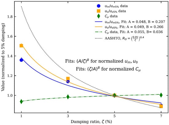
Figure 7. Comparison of normalized value of inelastic displacement, elastic displacement, and inelastic displacement ratio with the corresponding 5% damped value against AASHTO $R_D$. The normalized elastic displacement and inelastic displacement reduce with increase in damping as AASHTO $R_D$, while the inelastic displacement ratio increases with increase in damping ratio underlying the difference in damping effect in linear and nonlinear behavior.

The best-fit equations for damping reduction factor for elastic displacement ($R_{D\_elastic})$ and inelastic displacement ($R_{D\_inelastic}$) and amplification factor for inelastic displacement ratio $\left(A_D\right)$ were developed as a function of damping ratio $\zeta$. The equations are represented by Equations (27), (28) and (29), respectively.

$$R_{D\_elastic}={\left({\displaystyle \frac{0.048}{\zeta }}\right)}^{0.207}$$

(27)

$$R_{D\_inelastic}={\left({\displaystyle \frac{0.049}{\zeta }}\right)}^{0.266}$$

(28)

$$A_D={\left({\displaystyle \frac{\zeta }{0.055}}\right)}^{0.036}$$

(29)

Equations (27) and (28), derived from the full set of bridge analyses, offer more realistic estimates of elastic and inelastic displacement reduction factors than the conventional AASHTO $R_D$ equation, which was based on simplified single-degree-of-freedom (SDOF) systems without capturing the complexity of bridge-specific dynamics. Alternatively, Equation (29) can be used as damping amplification factor for the inelastic displacement ratio.

4. Conclusions and Recommendation

This study investigated the seismic behavior of six reinforced concrete (RC) box girder bridges by examining the relationship between earthquake-induced inelastic displacement ratios and the fundamental vibration periods of the structures. The analysis considered both pinned and fixed column-to-ground boundary conditions and applied 28 recorded ground motions from California over the past 55 years. Each earthquake’s two horizontal components were applied in the longitudinal and transverse directions of the bridge models. While bridge columns and abutments were modeled with nonlinear behavior to capture realistic seismic response, other components such as the superstructure deck and bent cap were modeled as elastic.

A key finding was that the inelastic displacement ratios based on mean values closely aligned with the AASHTO $R_d$ equation. However, the AASHTO equation was found to be inadequate in predicting inelastic displacement across the full spectrum of ground motions, revealing a significant limitation in its applicability. To improve predictive accuracy, additional equations were proposed. These formulations offer more robust estimates of inelastic displacement ratios under varying seismic conditions. The parametric analysis yielded several important conclusions:

• Column-to-Ground Connection: Bridges with pinned column bases exhibited higher inelastic displacement ratios than those with fixed connections. This is due to increased flexibility and rotational effects at the base, resulting in greater displacement demands.
• Column Height: As column height increased, inelastic displacement ratios also increased. Taller columns exhibit lower lateral stiffness, leading to larger displacements during seismic events.
• Deck Width: Although wider decks contributed to increased stiffness and reduced elastic displacements, their additional mass led to greater seismic forces, ultimately increasing inelastic displacement ratios.
• Number of Spans: While both elastic and inelastic displacements increased with the number of spans, the inelastic displacement ratio decreased. This indicates that multi-span bridges benefit from better load distribution and greater stiffness, reducing inelastic demands.
• Damping Ratio: Similarly to AASHTO guideline, the elastic and inelastic displacement decreased with increase in damping ratio; however, the inelastic displacement ratio increased with increase damping ratio representing the difference in damping effect in linear and nonlinear behavior of the bridges. To better reflect these behaviors, revised damping reduction factors for elastic and inelastic displacement and amplification factor for inelastic displacement ratio were suggested.

It is important to note that $T^{*}=1.25$ s has been considered in this research work, thus, the best-fit equations presented in this paper are applicable only to the bridge with a time period of the first mode less than 1.25 s. Equations (8) and (9) are suggested to be used instead of equation 4.3.3-1 of AASHTO Seismic Bridge Design Guide or equation 4.7.4.5-3 of AASHTO LRFD to satisfy the P-∆ requirement of the column or pier. Equation (8) gives response for moderate variation in ground motion while Equation (9) gives the upper bound estimate for a wide range of earthquake responses. Equations (27) and (28) are suggested to be used as damping reduction factor elastic and inelastic displacement instead of equation 4.3.2-1 of AASHTO Seismic Bridge Design Guide. Alternatively, Equation (29) can be directly used with the inelastic displacement ratio for damping other than 5%.

References

- Moehle, J.P. Displacement-based design of RC structures subjected to earthquakes. Earthq. Spectra 1992, 8, 403–428. [Google Scholar] [CrossRef]
- Whittaker, T.P.; Constantinou, M.; Tsopelas, P. Displacement estimates for performance-based seismic design. J. Struct. Eng. 1998, 124, 905–912. [Google Scholar] [CrossRef]
- Malekzadeh, H.; Eslamnia, H.; Moghadam, A.S. Probabilistic seismic demand modeling of continuous concrete box-girder bridges: Emphasizing hysteretic energy and residual demands. Adv. Bridge Eng. 2025, 6, 17. [Google Scholar] [CrossRef]
- Li, W.; Huang, Y.; Xie, Z. Machine Learning-Based Probabilistic Seismic Demand Model of Continuous Girder Bridges; Hindawi Publishing Corporation: London, UK, 2022. [Google Scholar]
- Zhang, J.; Yu SYTang, Y.C. Inelastic displacement demand of bridge columns considering shear-flexure interaction. Earthq. Eng. Struct. Dyn. 2011, 40, 731–748. [Google Scholar] [CrossRef]
- ATC. Tentative Provisions for the Development of Seismic Regulations for Buildings; Report ATC 3-06; ATC: Washington, DC, USA, 1978. [Google Scholar]
- ATC. Structural Response Modification Factors; Report ATC-19; ATC: Washington, DC, USA, 1995. [Google Scholar]
- Miranda, E. Evaluation of site-dependent inelastic seismic design spectra. J. Struct. Eng. 1993, 119, 1319–1338. [Google Scholar] [CrossRef]
- AASHTO. AASHTO LRFD Bridge Design Specifications, 10th ed.; American Association of State Highway and Transportation Officials: Washington, DC, USA, 2024. [Google Scholar]
- Rosenblueth, E.; Herrera, I. On a kind of hysteretic damping. J. Eng. Mech. Div. 1964, 90, 37–48. [Google Scholar] [CrossRef]
- Gulkan, P.; Sozen, M.A. Inelastic Responses of Reinforced Concrete Structure to Earthquake Motions. J. Proc. 1974, 71, 604–610. [Google Scholar]
- Iwan, W.D. Estimating inelastic response spectra from elastic spectra. Earthq. Eng. Struct. Dyn. 1980, 8, 375–388. [Google Scholar] [CrossRef]
- ATC. Seismic Evaluation and Retrofit of Concrete Buildings; Report ATC-40; ATC: Washington, DC, USA, 1996. [Google Scholar]
- Freeman, S.A. Evaluations of existing buildings for seismic risk-A case study of Puget Sound Naval Shipyard. In Proceedings of the 1st U.S. National Conference on Earthquake Engineering, Ann Arbor, MI, USA, 18–20 June 1975; Earthquake Engineering Research Institute: Berkeley, CA, USA, 1975. [Google Scholar]
- Freeman, S.A. Development and use of the capacity spectrum method. In Proceedings of the 6th U.S. National Conference on Earthquake Engineering, Seattle, WA, USA, 31 May–4 June 1998; Earthquake Engineering Research Institute: Oakland, CA, USA, 1998. [Google Scholar]
- Newmark, N.M.; Hall, W.J. Seismic Design Criteria for Nuclear Reactor Facilities. In Proceedings of the Fourth World Conference on Earthquake Engineering, Santiago, Chile, 13–18 January 1969; Volume II, pp. B4-37–B4-50. [Google Scholar]
- Miranda, E. Inelastic displacement ratios for structures on firm sites. J. Struct. Eng. 2000, 126, 1150–1159. [Google Scholar] [CrossRef]
- Miranda, E. Estimation of inelastic deformation demands of SDOF systems. J. Struct. Eng. 2001, 127, 1005–1012. [Google Scholar] [CrossRef]
- Rahnama, M.; Krawinkler, H. Effects of Soft Soil and Hysteresis Model on Seismic Demands; John, A., Ed.; Blume Earthquake Engineering Center Standford: Standford, CA, USA, 1993. [Google Scholar]
- Seneviratna, G.D.P.K.; Krawinkler, H. Evaluation of Inelastic MDOF Effects for Seismic Design; John, A., Ed.; Blume Earthquake Engineering Centre, Department of Civil Environmental Engineering, Stanford University: Standford, CA, USA, 1997. [Google Scholar]
- FEMA. NEHRP Guidelines for the Seismic Rehabilitation of Buildings; Reports FEMA 273 (Guidelines) and FEMA 274 (Commentary); FEMA: Washington, DC, USA, 1997.
- FEMA. Prestandard and Commentary for the Seismic Rehabilitation of Buildings; Report No. FEMA-356; FEMA: Washington, DC, USA, 2000.
- FEMA. Improvement of Nonlinear Static Seismic Analysis Procedures; Report No. FEMA 440; FEMA: Washington, DC, USA, 2005.
- Veletsos, A.S.; Newmark, N.M. Effect of inelastic behavior on the response of simple systems to earthquake motions. In Proceedings of the Second World Conference on Earthquake Engineering, Tokyo, Japan, 11–18 July 1960. [Google Scholar]
- Veletsos, A.S.; Newmark, N.M.; Chelapati, C.V. Deformation spectra for elastic and elastoplastic systems subjected to ground shock and earthquake motions. In Proceedings of the Third World Conference on Earthquake Engineering, Auckland-Wellington, New Zealand, 13–18 January 1965. [Google Scholar]
- Veletsos, A.S.; Vann, W.P. Response of ground-excited elastoplastic systems. J. Struct. Div. 1971, 97, 1257–1281. [Google Scholar] [CrossRef]
- Riddell, R. Statistical Analysis of the Response of Nonlinear Systems Subjected to Earthquakes; University of Illinois at Urbana-Champaign: Champaign, IL, USA, 1979. [Google Scholar]
- Ruiz-García, J.; Miranda, E. Inelastic displacement ratios for evaluation of existing structures. Earthq. Eng. Struct. Dyn. 2003, 32, 1237–1258. [Google Scholar] [CrossRef]
- Hatzigeorgiou, G.D.; Beskos, D.E. Inelastic displacement ratios for SDOF structures subjected to repeated earthquakes. Eng. Struct. 2009, 31, 2744–2755. [Google Scholar] [CrossRef]
- Wu, Y.-F.; Li, A.-Q.; Wang, H. Inelastic displacement spectra for Chinese highway bridges characterized by single-degree-of-freedom bilinear systems. Adv. Struct. Eng. 2019, 22, 3066–3085. [Google Scholar] [CrossRef]
- Bozorgnia, Y.; Mahmoud, M.H.; Kenneth, W.C. Deterministic and probabilistic predictions of yield strength and inelastic displacement spectra. Earthq. Spectra 2010, 26, 25–40. [Google Scholar] [CrossRef]
- AASHTO. AASHTO Guide Specifications for LRFD Seismic Bridge Design; American Association of State Highway and Transportation Officials: Washington, DC, USA, 2011. [Google Scholar]
- Martinez, D.R.; Kowalsky, M.J. Comparison of Seismic Demands on RC Bridge Columns Using the AASHTO Guide Specification, DDBA, and Nonlinear Analysis for Shallow Crustal and Subduction Tectonic Regimes. J. Bridge Eng. 2022, 27, 04022033. [Google Scholar] [CrossRef]
- NCHRP. Proposed Guidelines for Performance-Based Seismic Bridge Design; NCHRP Project 12-106; NCHPR: Washington, DC, USA, 2020. [Google Scholar]
- Aviram, A.; Mackie, K.R.; Stojadinović, B. Guidelines for Nonlinear Analysis of Bridge Structures in California; Pacific Earthquake Engineering Research Center: Berkeley, CA, USA, 2008. [Google Scholar]
- Omrani, R.; Mobasher, B.; Lian, X.; Gunay, S.; Mosalam, K.M.; Zareian, F.; Taciroglu, E. Guidelines for Nonlinear Seismic Analysis of Ordinary Bridges: Version 2.0; State of California Department of Transportation: Sacramento, CA, USA, 2015.
- Mackie, K.R.; Scott, M.H.; Johnsohn, K.; A-Ramahee, M.; Steijlen, M. Nonlinear Time History Analysis of Ordinary Standard Bridges California; Department of Transportation, Division of Engineering Services: Sacramento, CA, USA, 2017.
- Lu, J.; Elgamal, A.; Mackie, K.R. Parametric Study of Ordinary Standard Bridges Using OpenSees and CSiBridge; University of California: San Diego, CA, USA, 2015. [Google Scholar]
- Gyawali, B. Earthquake-Induced Inelastic Displacement Ratio in Reinforced Concrete Box Girder Bridges in California. Master’s Thesis, North Dakota State University, Fargo, ND, USA, 2024. [Google Scholar]
- Caltrans. Seismic Design Criteria Version 1.3; Caltrans: Sacramento, CA, USA, 2004.
- Caltrans. Seismic Design Criteria Version 1.7; Caltrans: Sacramento, CA, USA, 2013.
- Caltrans. Caltrans Seismic Design Criteria Version 2.0; Caltrans: Sacramento, CA, USA, 2019.
- Chopra, A.K. Dynamics of Structures: Theory and Applications to Earthquake Engineering, 3rd ed.; Prentice Hall: New Jersey, NJ, USA, 2006. [Google Scholar]
- Huff, T.; Pezeshk, S. Inelastic Displacement Spectra for Bridges Using the Substitute-Structure Method. Pract. Period. Struct. Des. Constr. 2016, 21, 04015020. [Google Scholar] [CrossRef]
Disclaimer/Publisher’s Note: The statements, opinions and data contained in all publications are solely those of the individual author(s) and contributor(s) and not of MDPI and/or the editor(s). MDPI and/or the editor(s) disclaim responsibility for any injury to people or property resulting from any ideas, methods, instructions or products referred to in the content. |
© 2025 by the authors. Licensee MDPI, Basel, Switzerland. This article is an open access article distributed under the terms and conditions of the Creative Commons Attribution (CC BY) license (https://creativecommons.org/licenses/by/4.0/).