Systematic Selection of Ground Motion Intensity Measures Satisfying the Probabilistic Seismic Demand Analysis

Abstract

In performance-based seismic design theory, the accurate selection of ground motion intensity parameters is crucial for the probabilistic assessment of structural seismic performance. To achieve efficient, sufficient, applicable, and complete prediction of structural seismic demands, this study systematically evaluates the comprehensive performance of 35 commonly used ground motion intensity measures (IMs). The research begins by analyzing 178 real records from the Pacific Earthquake Engineering Research Center (PEER) database, employing the Spearman rank correlation to reveal intrinsic relationships among the parameters. Subsequently, a ground motion database classified according to four site types based on Chinese seismic design codes is established. Combined with seven single-degree-of-freedom (SDOF) structural models of different periods, the performance of the IMs is comprehensively evaluated from four dimensions: correlation, efficiency, applicability, and completeness. Finally, by comparing the evaluation results under both bilinear and Clough stiffness-degrading bilinear hysteretic models, the robustness of the parameter selection is verified. The results demonstrate that: acceleration-related parameters are most suitable for short-period structures, velocity-related parameters for medium-period structures, and displacement-related parameters for long-period structures. Parameters Sv_avg and Sd_avg exhibit consistent performance across all period ranges and under different site conditions, and the evaluation results remain consistent across different hysteretic models. This study provides a systematic basis for the rational selection of intensity parameters in probabilistic seismic demand analysis, significantly enhancing the reliability and precision of seismic performance assessment.

1. Introduction

Probabilistic seismic demand analysis [1,2,3] incorporates two key variables—a structural performance parameter and a ground motion intensity measure [4,5]—to assess seismic damage and structural response. Establishing a robust correlation between these variables is essential for accurate seismic performance evaluation and the reduction in response prediction variability. However, under earthquakes beyond the design basis—characterized by higher intensity, longer duration, and stronger nonlinear effects—conventional intensity measures may fail to reliably predict structural behavior, potentially leading to progressive collapse. Recent research has prioritized enhancing structural resilience through innovative methodologies, including the implementation of self-centering components, damage-mitigation strategies for irregular joints and composite frames, and material improvements incorporating modified fibers to enhance crack resistance [6,7,8,9,10]. These approaches collectively contribute to maintaining functional integrity under extreme conditions. In this context, selecting optimal intensity measures that are closely related to structural seismic demand becomes critically important for advancing performance-based design under extreme seismic scenarios.

Currently, numerous parameters for ground motion intensity have been proposed as evaluation indices for structural damage. These parameters can be categorized into three types based on the three elements of ground motion, namely, amplitude, frequency spectrum, and duration.

(1) Intensity parameters related to the amplitude of ground motion

The accuracy of seismic input directly determines the reliability of probabilistic seismic demand analysis (PSDA), while various factors in actual sites can distort the original characteristics of seismic signals [11]. The intensity parameters are typically obtained by calculating seismic motion time histories and represent the non-structural characteristics of the seismic motion intensity. They generally refer to the average or maximum values of physical quantities such as acceleration, velocity, and displacement in seismic records. For instance, the Chinese Code for Seismic Design of Buildings [12] uses the peak ground acceleration (PGA), Japanese regulations use the peak ground velocity (PGV), and researchers have studied the peak ground displacement (PGD). Additionally, other parameters such as the Arias intensity (I_A) [13], which measures the total duration and amplitude of an earthquake, the Riddell indices (I_a, I_v, and I_d) [14], which are applicable to structures with different periods and ductilities, the characteristic intensity (I_C) [15], which describes the relationship between structural damage and seismic intensity, and the Fajfar intensity index (I_F) [16], among others, should also be considered.

(2) Intensity parameters related to the frequency spectrum of ground motion

This type of ground intensity parameter is calculated based on the structural period and is related to the structural characteristics derived from the seismic response spectrum of the ground motion. For complex seismic motions, they can be decomposed into multiple harmonic waves with different amplitudes and frequencies. These harmonic waves can be plotted in a frequency–amplitude coordinate system to obtain the spectrum. When the natural frequency of the building structure is close to the dominant frequency of the seismic motion, the structure will experience a larger response. Scholars have proposed intensity parameters related to the seismic response spectrum, such as peak spectral acceleration (PSA), peak spectral velocity (PSV), and peak spectral displacement (PSD) [17]. They have also introduced acceleration spectrum intensity (ASI), velocity spectrum intensity (VSI), and displacement spectrum intensity (DSI) [18].

(3) Intensity parameters related to earthquake duration

The duration of an earthquake, as one of the three essential components of seismic motion, has an impact on structures that is reflected in the cumulative damage effects of the earthquake. Xie and Zhang [19] categorized earthquake duration into two types: duration unrelated to structural characteristics and engineering duration related to structural characteristics. Bolt [20] defined “bracket duration” as the time taken for the absolute value of the recorded ground motion acceleration to first reach or exceed a specified threshold and the time taken for it to reach or fall below the threshold for the last time. Trifunac and Brady [21], based on the relative energy of the earthquake motion, defined “important duration” as reflecting the energy distribution throughout the entire earthquake motion process.

Researchers have conducted a series of studies in order to reduce the uncertainty in predicting the seismic demand of structures within the framework of performance-based probabilistic seismic engineering methods by selecting appropriate intensity parameters.

Jayaram et al. [22] investigated the correlation between the maximum structural response and intensity parameters in concrete frame structures and found that the correlation between deformation-based response and intensity parameters related to velocity is better than that of force-based response. Bianchini et al. [23] used the average acceleration response spectrum Sa_avg(T₁,…,T_n) to predict the elastic–plastic response of buildings under earthquake ground motion. The results showed that Sa_avg(T₁,…,T_n) had a stronger predictive ability than the first-period spectral acceleration S_a(T₁) and the peak ground acceleration (PGA). Tajammolian et al. [24] investigated the effects of peak ground velocity (PGV) of the near-field pulses on responses of base-isolated structures employing different types of friction isolators and found that increasing the PGV causes the structure responses to rise. The results showed that PGV is more closely related to deformation demands compared to other measures of ground motion intensity. Shome [3] analyzed the maximum response of a five-story four-span building structure subjected to ground motion and found that the first periodic spectral acceleration Sa(T₁) exhibited a stronger correlation than peak ground acceleration (PGA). Giovenale et al. [25] also reached a similar conclusion. However, some studies argue that estimating the fundamental period of the structure when calculating Sa(T₁) may introduce errors [3,26]. Yakut and Yilmaz [27] investigated the correlation between the maximum inter-story displacement requirement of frame structures and ground motion intensity parameters. The research revealed that the correlation of spectrum intensity parameters was better than that of other parameters, such as PGV and PGA. Konstantinos et al. [28] investigated some advanced ground motion intensity measures (IMs) to predict the structural damage of earthquake-resistant 3D R/C buildings and found that spectral acceleration is a relatively good IM for medium-rise R/C buildings that possess small structural eccentricity. Early scalar intensity measures (IMs), which neglected spectral shape sensitivity, led to significant variability in predicting the responses of multi-degree-of-freedom structures [29]. In response, scholars introduced vector IMs, such as (Sa(T₁), ε), where ε quantifies deviations in spectral shape, thereby markedly enhancing sufficiency. Tothong and Luco [30] proposed IMs incorporating higher-mode modifications, addressing the underestimation of higher-mode effects in long-period structures. Luco and Cornell [31] considered second-order frequency components and nonlinearity, proposing the use of suitability and completeness indices to evaluate seismic intensity parameters, both of which can be quantified. Furthermore, the average spectral acceleration proposed by Eads et al. [32] demonstrated consistent efficiency across structures with varying periods, confirming that period dependency is a fundamental criterion in intensity measure selection. Konstantinos [33] investigated the role of the masonry infills on the correlation between widely used ground motion intensity measures (IMs) and the damage state of 3D R/C buildings. The results indicated that the distribution of masonry infill strongly influences the correlation between IM and seismic damage. Takewaki and Tsujimoto [34] investigated the relationship between seismic intensity normalization indices, such as acceleration power and velocity power, with response performance (peak inter-story drift, total input energy). The results showed that when velocity power is used as the normalization index, the total input energy exhibits a stable characteristic independent of the number of layers. Liu et al. [35] investigated the influence of intensity measure selection on the seismic response of bridge structures. Their findings revealed that choosing the right intensity measure is crucial for predicting bridge damage under different seismic scenarios, especially in complex bridge configurations, highlighting the importance of selecting appropriate IMs for accurate damage assessment. Xu et al. [36] compared response-based and demand-based intensity measures for seismic fragility analysis of buildings. The study demonstrated that demand-based IMs, particularly those incorporating displacement measures, provide a more accurate prediction of building damage and performance, offering a better tool for fragility analysis.

The dynamic time-history analysis of six reinforced concrete frame-core tube long-period structures, conducted by Guan et al. [37], revealed that peak ground velocity and peak ground displacement are optimal for such structures. Osei and Adom-Asamoah [38] investigated the sufficiency of the mean spectral acceleration with respect to the ground motion time history. The results suggest that the sufficiency of mean spectral acceleration may improve as the period of the single-degree-of-freedom system increases, compared to Sa(T₁). Pejovic et al. [39] proposed a new intensity measure and used it for probabilistic seismic analysis of RC high-rise buildings with core wall structures. The research results showed that the newly proposed strength parameter can effectively predict seismic motion intensity with minimal dispersion and satisfactory practicality. Zhang et al. [40] conducted a study on the relationship between ground motion parameters and the seismic response of slopes. Their findings indicated that PGV can be considered the most suitable parameter for analysis. Torres et al. [41] utilized the generalized intensity measure INpg to predict the efficiency of peak floor acceleration demands in steel frame buildings under seismic excitation. The results indicate that it can effectively enhance the predictive efficiency of structural nonlinear behavior under seismic actions. Zhong et al. [42] proposed a scalar intensity measure (IM) for assessing the seismic response of single-layer reticulated domes and compared its applicability and superiority with 11 other existing IMs. The results indicated that this IM exhibits strong correlation, high efficiency, and good sufficiency relative to the other IMs. Yakhchalian et al. [43] proposed a novel parameter known as gamma (γ), which serves as an effective indicator for selecting ground motion in earthquake collapse assessment for high-rise buildings. Li et al. [44] classified ground motion intensity parameters into four categories: type I, represented by Sa(T₁); type II, represented by PGA; type III, represented by PGD; and type IV, represented by PGV. The findings revealed a strong correlation between type I intensity parameters and various periodic structures, suggesting that they should be considered as the index for ground motion intensity. Ko and Ha [45] conducted a study on the optimal measurement of seismic intensity for shaking foundations among 15 seismic intensity parameters. The results showed that peak ground velocity is an effective predictor of the seismic performance of shaking foundations. Armstrong et al. [46] analyzed the best intensity measures that are related to deformations of embankment dams. The study found that Arias intensity (I_A) was the most effective IM for predicting embankment dam deformations. Wu et al. [47] conducted a study aimed at identifying the most effective scalar- and vector-valued intensity measures for predicting liquefaction triggering. They determined that the acceleration spectrum intensity (ASI) and the vector of peak ground acceleration and spectral acceleration at 0.3 s are the optimal scalar- and vector-IMs for evaluating liquefaction triggering. Padgett et al. [48] conducted a study to evaluate the optimal intensity measures for generating probabilistic seismic demand models for bridge portfolios. The results of their study revealed that cumulative absolute velocity is the most optimal IM when using recorded motions. Chen et al. [49] proposed a new scalar ground motion intensity measure called the energy–frequency parameter based on the Hilbert–Huang transform. The efficiency results demonstrate a strong linear correlation between the energy–frequency parameter and the engineering demand parameter (EDP) on a natural logarithmic scale, which applies to various structural fundamental periods. Flores et al. [50] investigated the influence of strong ground motion duration on the probability of collapse of reinforced concrete walls. The results revealed that, compared to short-duration ground motion sets, long-duration ground motion sets decreased the average collapse capacity of medium-to-long period walls. In recent years, the development of IMs has started to focus on multimodal effects. Muho et al. [51] and Kalapodis et al. [52] have proposed spectral acceleration- and displacement-based IMs that incorporate higher-mode effects and performance levels through equivalent modal damping ratios.

In previous studies on the correlation analysis of seismic intensity measures (IMs), several limitations persist: the use of restricted ground motion datasets often overlooks the influence of site conditions; the number of IMs considered is frequently limited; and the effect of structural hysteresis models on IM evaluation is seldom addressed. To address these gaps, this study conducts a comprehensive correlation analysis of 35 IMs. A site-specific ground motion database is established, categorizing records into four distinct site types, acknowledging the critical role of local soil conditions as emphasized in hysteretic energy studies. The IM performance is evaluated under seismic inputs representative of each site type using four criteria—correlation, efficiency, applicability, and completeness—applied to single-degree-of-freedom systems with seven natural periods. This systematic approach yields comprehensive IM evaluations across different structural period ranges. Furthermore, a comparative analysis is performed between results derived from bilinear and degraded bilinear hysteresis models. This comparison elucidates the influence of hysteretic behavior on IM selection and performance, thereby providing deeper insight into their robustness for performance-based seismic design.

2. Selection of Ground Motion Intensity Parameters and Ground Motion Acceleration Records

2.1. Existing Ground Motion Intensity Parameter Index

Obviously, it is not reasonable to describe the intensity of an earthquake solely using a single parameter indicator, as it would overlook a vast amount of seismic information. Riddell [53] proposed using a time function $f(t)$ to represent the intensity parameter of ground motion.

$$f_{peak}=\max (\left|f(t)\right|)$$

(1)

$$f_{sum}={\displaystyle {\int }_{t_1}^{t_2}f(t)dt}$$

(2)

$$f_{sum}^{abs}={\displaystyle {\int }_{t_1}^{t_2}\left|f(t)\right|}dt$$

(3)

$$f_{avg}={\displaystyle \frac{1}{t_2-t_1}}{\displaystyle {\int }_{t_1}^{t_2}f(t)dt}$$

(4)

where $t\subseteq [0,t_{tot}]$, $t_{tot}$ is the total duration of the earthquake; $t_1$ and $t_2$ represent specific durations, $t_1<t_2$.

If $f(t)$ is oscillatory, it can be defined as:

$$f_{sum}^{sqr}={\displaystyle {\int }_{t_1}^{t_2}{(f(t))}^{2}dt}$$

(5)

$$f_{avg}^{sqr}={\displaystyle \frac{1}{t_2-t_1}}{\displaystyle {\int }_{t_1}^{t_2}{(f(t))}^2}dt$$

(6)

For $f(t)$, a single indicator can be obtained by integrating the total earthquake duration from $t_0$ to $t_{tot}$, or it can be integrated from $t_1$ to $t_2$ within a specific time range to obtain some comprehensive quantities.

According to Riddell’s research, when the displacement, velocity, and acceleration response spectra of a structure are unified in a three-logarithmic coordinate system, a new tripartite response spectrum can be obtained, as shown in Figure 1.

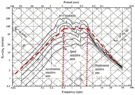
Figure 1. Example of tripartite response spectrum.

In the new coordinate system, the three types of seismic response spectra have a constant cross-section at different periods, corresponding to short-period, mid-period, and long-period, respectively. The different period ranges correspond to the acceleration/velocity/displacement-sensitive region. Based on this, the seismic intensity parameter indicators are divided into the following: acceleration-related type, velocity-related type, displacement-related type, and other types.

The present study selected 35 representative and commonly used parameters of ground motion as research subjects, as shown in Table 1.

Table 1. Classification and summary of ground motion intensity parameters.

Category	Numbering	Earthquake Intensity Parameter Name	Symbol
Acceleration related type	1	Ground motion peak ground acceleration	PGA
	2	Cumulative absolute velocity	CAV
	3	Pseudo-spectral acceleration	PSA
	4	Acceleration response spectrum mean	Saavg
	5	Effective peak acceleration	EPA
	6	Acceleration-type spectral intensity	ASI
	7	Arias intensity	IA
	8	Square-root acceleration	Ars
	9	Root-mean-square acceleration	Arms
	10	Characteristic intensity	IC
	11	Riddell index-Ia	Ia
Velocity related type	12	Ground motion peak ground speed	PGV
	13	Cumulative absolute displacement	CAD
	14	Peak spectral velocity	PSV
	15	Velocity response spectrum mean	Svavg
	16	Effective peak velocity	EPV
	17	Velocity-type spectral intensity	VSI
	18	Modified Arias intensity	IA,M
	19	Square root velocity	Vrs
	20	Root mean square velocity	Vrms
	21	Fajfar intensity	IF
	22	Housner spectral intensity	IH
	23	Riddell index-Iv	Iv
Displacement related type	24	Ground motion peak ground displacement	PGD
	25	Cumulative absolute momentum	CAI
	26	Peak of spectral displacement	PSD
	27	Displacement response spectrum mean	Sdavg
	28	Effective peak displacement	EPD
	29	Displacement-type spectral intensity	DSI
	30	Square root displacement	Drs
	31	Root mean square displacement	Drms
	32	Riddell index-Id	Id
Other types	33	Ground motion peak velocity to acceleration ratio	FR1
	34	Ground motion peak displacement to velocity ratio	FR2
	35	Strong earthquake duration	TD

Note: $CAI={\displaystyle {\int }_0^{{{\displaystyle t}}_f}\left|u_g(t)\right|}dt$, which is an intensity measure parameter obtained by integrating the absolute value of the ground motion displacement time history over the entire earthquake duration. $Ars=\sqrt{{\displaystyle {\int }_0^{t_f}{\stackrel{••}{u}}_g^2}(t)dt}$, $A_{rms}=\sqrt{{\displaystyle \frac{{\int }_{t_1}^{t_2}{\stackrel{••}{u}}_g^2(t)dt}{t_2-t_1}}}$, $F{R}_2={\displaystyle \frac{PGD}{PGV}}$, $F{R}_1={\displaystyle \frac{PGV}{PGA}}$.

2.2. Selection of Ground Motion Acceleration Records

Three main factors are considered in the selection of ground motion acceleration: ground motion magnitude, epicenter distance, and site type (equivalent shear wave velocity V_s30). According to the literature [54], the ground motion records of site types corresponding to Chinese specifications are selected according to V_s30. The selection principles are as follows:

• Earthquake magnitude Mw > 5.5.
• The distance between the epicenter and R is greater than 0 km and less than 100 km.
• In the Chinese seismic design code, when V_S30 > 510 m/s, it corresponds to class I site; when 510 m/s > V_S30 > 260 m/s, it corresponds to class II site; when 260 m/s > V_S30 > 150 m/s, it corresponds to class III site; when V_S30 < 150 m/s, it corresponds to class IV site.

According to the above principles, 178 original ground motion records were selected from the PEER earthquake database NGA-West2 (PEER, 2013; data accessed on 15 March 2020). Figure 2a–d provide specific distributions of the selected ground motion records in terms of magnitude, epicentral distance, and soil equivalent shear wave velocity. Overall, the selected ground motion records exhibit a broad distribution in terms of magnitude, epicentral distance, and site type, ensuring that records with different seismic motion characteristics are encompassed.

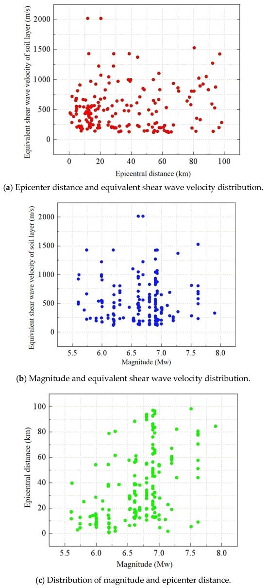
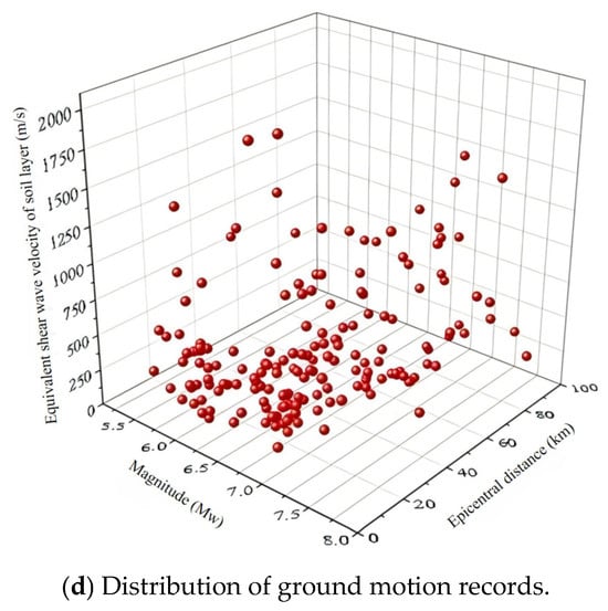
Figure 2. Distributions of the selected ground motion records in terms of magnitude, epicentral distance, and soil equivalent shear wave velocity.

2.3. Research on the Correlation Between Ground Motion Intensity Parameters

Each parameter index of ground motion intensity represents a specific characteristic of ground motion. These parameters can either be independent of each other or exhibit a strong correlation. To assess the level of correlation between the studied parameters, the Spearman rank correlation coefficient is employed.

The Spearman rank correlation coefficient can effectively describe the correlation between two variables X and Y, and its value ranges from −1 to 1. A value of 1 or −1 indicates that each variable is a strictly monotonic function of the other variable, while a value of 0 indicates no correlation between the two variables. The Spearman rank correlation coefficient between two variables X and Y is calculated using Equation (7):

$${\rho }_{\mathrm{Spearman}}=1-{\displaystyle \frac{6{\displaystyle {\sum }_{i=1}^N{D_{\mathrm{i}}}^2}}{N(N^2-1)}}$$

(7)

where D_i represents the difference between the ranks of each pair of observations for the two variables, and N represents the total number of data points (X, Y).

Using MATLAB (R2024b), the Spearman rank correlation coefficients between 35 intensity parameter indicators were calculated for 178 seismic records using Equation (7). The calculation results can be found in Appendix Table A1. A heatmap of the Spearman rank correlation coefficients was also plotted, as shown in Figure 3.

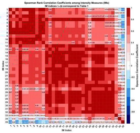
Figure 3. Thermal map of Spearman rank correlation coefficient of ground motion intensity parameters.

Figure 3 illustrates the Spearman rank correlation matrix among 35 ground motion intensity measures (IMs), visually summarizing their statistical interdependencies through a color-gradient heatmap. The plot distinctly depicts strong positive correlations (indicated by dark red cells, approaching +1.0) among certain IMs, forming visible high-correlation clusters along the diagonal and off-diagonal regions. In contrast, light blue to dark blue cells (ranging toward –1.0) reflect negative correlations, highlighting IM pairs that convey complementary rather than redundant information. The Spearman rank correlation analysis of each intensity parameter reveals that, among the peak ground acceleration (PGA), peak ground velocity (PGV), and peak ground displacement (PGD), PGV and PGD have a stronger correlation with the other intensity parameters compared to PGA. The square root of the peak ground velocity (V_rs) is most correlated with the mean response spectrum value (Sv_avg). I_A and A_rs; EPD and DSI; EPA and ASI; and EPV, VSI, and I_H are highly correlated with each other and may indicate that they possess similar capabilities in characterizing ground motion intensity. Time-related intensity parameters (FR₁, FR₂, T_D) exhibit relatively low correlations with other parameters. Although some of these correlations exceed 60%, they remain significantly lower than those of other types of IMs.

3. Statistical Analysis of Structural Response and Ground Motion Intensity Parameters Under Different Site Types

3.1. Probabilistic Seismic Demand Analysis

Probabilistic seismic demand analysis plays a crucial role in the analysis of structural seismic vulnerability. It involves conducting a nonlinear time-history analysis of a structure’s dynamic response to seismic excitations using either the cloud image method or incremental dynamic analysis (IDA). The conditional probability relationship between the structure reaching or exceeding the prescribed seismic demand (DM) level and a certain ground motion intensity is determined under these conditions. The conditional probability described in Equation (8) is referred to as the structural probabilistic seismic demand model.

$$P_D=P\left[D\ge d|IM\right]$$

(8)

In previous research [55], it was assumed that the structural probability seismic demand follows a lognormal distribution. This assumption was verified by conducting tests. The maximum deviation between the hypothetical cumulative lognormal distribution and the observed cumulative distribution was calculated using the following equation:

$$F={\max }_{i=1}^n[|F^{\ast }(X_i)-F_X(X_i)|]$$

(9)

where $F^{\ast }(X_i)={\displaystyle \frac{i}{n}}$; n is the number of samples; and $F_X(X_i)=CDF$ is the cumulative distribution function of the lognormal distribution. The testing results indicate that the hypothesis is valid.

When assuming that the seismic probability demand (DM) of the structure follows a lognormal distribution, a study by Cornell et al. [56] demonstrated that the relationship between the median position ($\stackrel{\wedge }{D}$) of the DM and the ground motion intensity can be described by the following exponential relationship,

$$\stackrel{\wedge }{D}=aI{M}^b$$

(10)

where a and b are regression parameters, determined through regression analysis. By simplifying Equation (10), we obtain the following formula,

$$\mathrm{In}\stackrel{\wedge }{D}=b\mathrm{In}(IM)+\mathrm{In}(a)$$

(11)

In the logarithmic conversion space, the logarithmic structure requirement lnD obeys the normal distribution, where the median value is $\ln \stackrel{\wedge }{D}$, and the standard deviation is marked σ, which is an estimate of the conditional logarithmic standard deviation ${\beta }_{D|IM}$,

$${\beta }_{D|IM}=\sqrt{{\displaystyle \frac{{\displaystyle \sum {[\mathrm{In}(d_i)-\mathrm{In}(aI{M}_i^b)]}^2}}{N-2}}}$$

(12)

where $d_i$ is the seismic demand of the structure under the i-th ground motion, and $I{M}_i$ is the i-th ground motion intensity. Substituting Equations (10)–(12) into Equation (8), the probabilistic seismic demand model based on log-linear regression can be derived.

$$P[D\ge d|IM]=1-\mathsf{\Phi }\left({\displaystyle \frac{\mathrm{In}d-\mathrm{In}(aI{M}^b)}{{\beta }_{D|IM}}}\right)=\mathsf{\Phi }\left({\displaystyle \frac{\mathrm{In}(IM)-\frac{[\mathrm{In}(d)-\mathrm{In}(a)]}{b}}{\frac{{\beta }_{D|IM}}{b}}}\right)$$

(13)

In general, the basic assumptions of the structural probabilistic seismic demand model comprise the following three aspects:

(1)

Under the condition of ground motion intensity $IM=x$, the seismic demand D of structures is usually assumed to follow a lognormal distribution.

(2)

There exists a logarithmic linear relationship between the median value of structural seismic demand $\stackrel{\wedge }{D}$ and IM.

(3)

${\beta }_{D|\mathrm{IM}}$ remains constant regardless of the change in IM.

The relationship between structural seismic probability requirements and ground motion intensity parameters in this paper is established on the aforementioned assumptions.

3.2. Ground Motion Classification Based on Site Type

The classification standards for site types in Chinese and American codes differ, as indicated in Table 2 and Table 3. Nevertheless, there is no discrepancy in terms of how the same site conditions impact ground motion.

According to the research by Lü [57], 178 seismic acceleration records from the PEER database were selected and classified according to the following principles.

• When V_S30 > 510 m/s, it corresponds to class I sites in the Chinese seismic code; and when V_S30 > 800 m/s, it corresponds to class I subclasses in the Chinese seismic code, including class A sites, class B sites, and some class C sites in the American code.
• When 510 m/s > V_S30 > 260 m/s, it corresponds to a class II site in the Chinese seismic code, including a class C site and class D site in the American code.
• When 260 m/s > V_S30 > 150 m/s, it corresponds to class III sites in the Chinese seismic code, including class D sites and some class E sites in the American code.
• When V_S30 < 150 m/s, it corresponds to a class IV site in the Chinese seismic code, including a class E site in the American code.

Table 2. American IB2006 site classification standard [58].

Site	General	Classification Index
Category	Description	Vs30(m/s)	${\overline{N}}_{SPT}$	${\overline{s}}_u(\mathrm{kPa})$
A	Hard rock	>1500	-	-
B	Rock	760~1500	-	-
C	Hard soil	360~760	>50	>100
D	Medium hard soil	180~360	15~50	50~100
E	Soft soil	≦180	<15	<50
		Soft soil with H > 3 m:PI > 20, W > 40%,
F	-	F1: Easily collapsible or destructible highly sensitive clay, with poor cohesive properties.
		F2: Argillaceous soil or high organic clay, H > 3 m
		F3: High plastic clay, PI > 20, H > 8 m
		F4: Very thick soft-medium hard clay, H > 36 m

H: the thickness of overburdened soil; PI: the plasticity index; W: the water content.

Table 2. American IB2006 site classification standard [58].

Site	General	Classification Index
Category	Description	Vs30(m/s)	${\overline{N}}_{SPT}$	${\overline{s}}_u(\mathrm{kPa})$
A	Hard rock	>1500	-	-
B	Rock	760~1500	-	-
C	Hard soil	360~760	>50	>100
D	Medium hard soil	180~360	15~50	50~100
E	Soft soil	≦180	<15	<50
		Soft soil with H > 3 m:PI > 20, W > 40%,
F	-	F1: Easily collapsible or destructible highly sensitive clay, with poor cohesive properties.
		F2: Argillaceous soil or high organic clay, H > 3 m
		F3: High plastic clay, PI > 20, H > 8 m
		F4: Very thick soft-medium hard clay, H > 36 m

H: the thickness of overburdened soil; PI: the plasticity index; W: the water content.

Table 3. Criteria for site classification in China seismic design code [12] (Ministry of Housing and Urban-Rural Development, PRC 2016).

Shear Wave Velocity of Rock or the Equivalent Shear Wave of Soil (m/s)	Site Category
	I0	I1	II	III	IV
Vs > 800	0
800 ≥ Vs > 500		0
500 ≥ Vse > 250		<5	≥5
250 ≥ Vse > 150		<3	3~50	>50
Vse < 150				15~80	>80

V_s: shear wave velocity of rock.

Table 3. Criteria for site classification in China seismic design code [12] (Ministry of Housing and Urban-Rural Development, PRC 2016).

Shear Wave Velocity of Rock or the Equivalent Shear Wave of Soil (m/s)	Site Category
	I0	I1	II	III	IV
Vs > 800	0
800 ≥ Vs > 500		0
500 ≥ Vse > 250		<5	≥5
250 ≥ Vse > 150		<3	3~50	>50
Vse < 150				15~80	>80

V_s: shear wave velocity of rock.

According to the aforementioned principles, the 178 selected ground motion records are classified into four categories based on the site type. With the exception of the category IV site, which includes only 18 ground motion records, all other site types consist of 40 ground motion records each. Within these site types, the ground motion record database for a category I site is further subdivided into two subcategories: I₀ and I₁ (refer to Table A2, Table A3, Table A4, Table A5 and Table A6 in the Appendix A). Figure 4a–e, respectively, show the acceleration response spectrum curves of the damping ratio $\xi =5\%$ of the ground motion recording library of different site types in logarithmic coordinates.

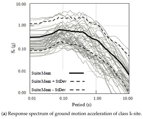
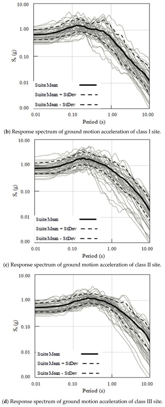
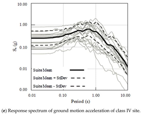
Figure 4. Acceleration response spectrum curves of different site types.

3.3. Statistical Analysis Based on Evaluation Criteria of Ground Motion Intensity Parameter

This study selects the maximum structural displacement U_max as the parameter to investigate the statistical relationships with ground motion intensity measures (IMs). Building upon existing research, the most commonly used criteria of correlation, efficiency, applicability, and completeness are selected as the evaluation principles for the rational selection of IMs.

In this section, we conduct a nonlinear elastic–plastic dynamic time-history analysis of a single-degree-of-freedom structural system (Figure 5) using the Clough stiffness-degrading bilinear hysteretic model (Figure 6).

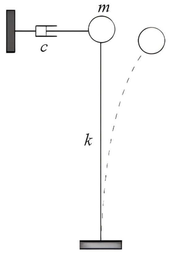
Figure 5. Schematic diagram of single-degree-of-freedom system.

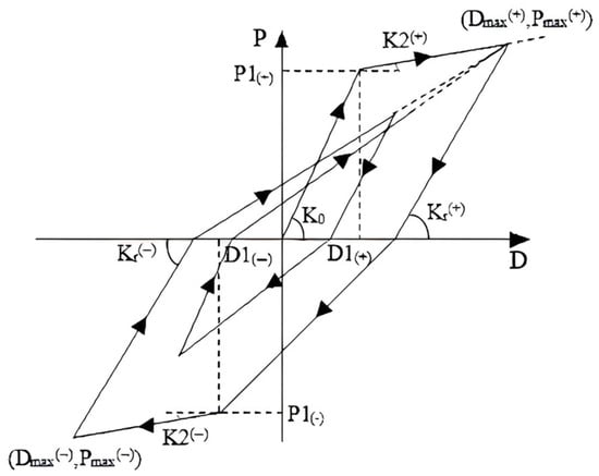
Figure 6. Clough stiffness-degrading bilinear hysteretic model.

In the nonlinear elastic–plastic SDOF structure system, the initial stiffness is denoted as K₀ = 100 kN/m. The damping ratio is denoted as $\zeta =5\%$. The post-yield stiffness reduction factor is denoted as $\alpha =0.1$. The ductility factor is denoted as μ = 3.0. The natural vibration periods of the structural system models are chosen as T = 0.5 s, 1 s, 2 s, 3 s, 4 s, 5 s, and 6 s. These models represent seven single-degree-of-freedom (SDOF) structural systems with varying natural vibration periods. This paper divides the duration of 0.5 s into the short-period range, 1 to 3 s into the intermediate period range, and 4 to 6 s into the long-period range. This model covers three different structural types with three different periods, and it represents the period ranges of the acceleration/velocity/displacement-sensitive regions in tripartite response spectra.

3.4. Statistical Results of Correlation and Analysis

The correlation refers to the strength of the relationship between the ground motion intensity parameters and the structural demand parameters. A stronger correlation means that the intensity measure can better predict the structural response, and thus can be considered an effective measure of intensity. We examine the relationship between the maximum seismic response (DM) of a single-degree-of-freedom (SDOF) elastic–plastic system and ground motion intensity measures (IMs), using the maximum structural displacement response U_max as a representative index for the structural response. The analysis steps are as follows:

(1)

Using the Bispec2.20 software (Version 2.20), perform elastoplastic nonlinear dynamic time-history analysis on SDOF systems with different periods to calculate DM_i for the i-th ground motion record.

(2)

For the i-th ground motion acceleration record, calculate the corresponding IM_i (a total of 35 intensity parameters).

(3)

To obtain the data points (IM_i, DM_i) for the i-th seismic input, plot them in a ln(IM) − ln(DM) coordinate system, and perform linear regression on the data points.

(4)

Analysis of goodness of fit for curve fitting is performed by evaluating the adjusted coefficient of determination, denoted as R². The greater the value of R², the better the fit, indicating a stronger correlation.

(5)

Alter the structural period and repeat the above steps to obtain the correlation between the ground motion intensity measures of 35 ground motion records and U_max at various periods for different types of sites.

Taking PGV as an example, the correlation analysis between ground motion intensity parameters and structural response under site type I₀ at T = 0.5 s is illustrated in Figure 7.

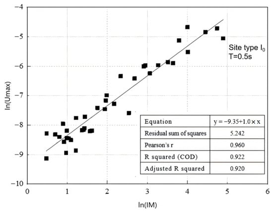
Figure 7. Evaluation of the correlation between IM and U_max.

According to the described steps, we obtained the discriminatory coefficient R² for 35 ground motion intensity parameters under different structural periods and different site type seismic inputs (see Appendix Table A7). Based on R², we plotted the correlation graph between U_max and IMs, as shown in Figure 8.

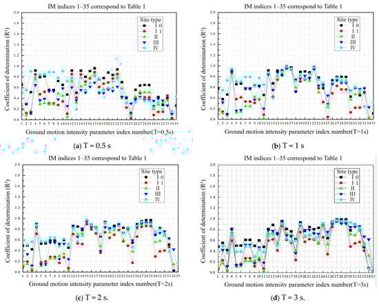
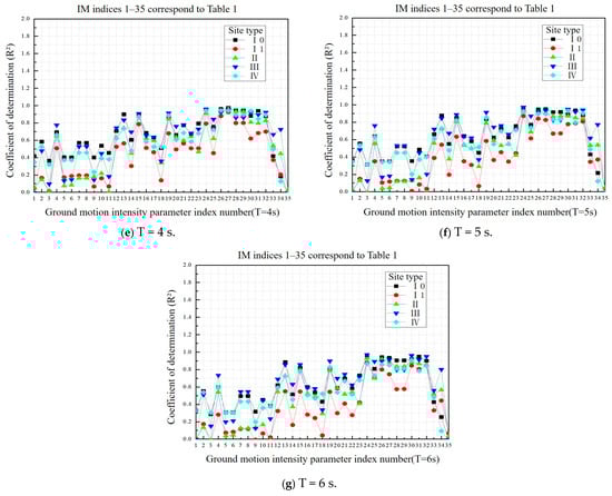
Figure 8. Comparison of the coefficient of determination (R²) of ground motion intensity parameters under different site types.

Through comparative analysis, we found the correlation of intensity parameters associated with acceleration is relatively high in the short-period range, but this correlation varies significantly across different site types and decreases as the structure’s period increases. In the mid-period range, the correlation of intensity parameters related to velocity is higher. However, as the structure’s period increases, the correlation of the same intensity parameter in different sites becomes more variable. In contrast, the correlation of intensity parameters associated with displacement shows a rapid increase as the structure’s period increases, and their correlation is less influenced by the site type.

Correlation analysis shows that peak ground velocity (PGV) is effective for short-period structures, whereas peak ground displacement (PGD) is more appropriate for long-period structures. This difference arises from the inherent relationship between the frequency content of ground motions and the dynamic properties of structures. Short-period structures, which are stiffer, have responses primarily controlled by inertial forces. PGV effectively reflects the mid-to-high frequency energy of ground motions, matching the sensitive frequency range of short-period structures. Conversely, long-period structures are highly flexible, and their failure is often dominated by global deformation. PGD directly captures the low-frequency energy of ground motions, which is physically consistent with the deformation demands of long-period structures, leading to stronger correlations. It should be noted that although PGV is generally an excellent intensity measure (IM) for short-period structures, this does not preclude the possibility that other parameters may perform better at specific period points. As shown in Appendix Table A7, at T = 0.5 s, the velocity spectrum intensity (VSl) exhibits a slightly higher correlation (R² = 0.96) than PGV (R² = 0.92). The reason for this is that VSI, as a velocity-based spectral intensity parameter, integrates velocity spectra over a specific period range, thereby containing richer frequency information compared to the single-peak value of PGV. At the specific period of T = 0.5 s, VSI may more accurately capture the seismic energy near that period, thus establishing a stronger correlation with structural response.

3.5. Statistical Results of Efficiency and Analysis

Efficiency refers to the ability of an intensity measure (IM) to predict the engineering demand parameters. An effective IM should be able to capture the key characteristics of the ground motion and be correlated with critical structural performance indicators. The logarithmic standard deviation ${\beta }_{D|IM}$ is used as the evaluation index for efficiency. Smaller values of ${\beta }_{D|IM}$ indicate better corresponding ground motion parameters. The calculation method of ${\beta }_{D|IM}$ can be determined using Equation (12).

The selected probabilistic earthquake demand model in this paper is Equation (8), which does not account for errors attributable to mathematical assumptions. In Section 3.4, a total of 1225 regression models were derived to analyze 35 ground motion intensity parameters across four site types and seven different structural periods (due to space constraints, the detailed list of models is not provided). The validity, applicability, and completeness analysis in this section are all based on these 1225 regression models.

The efficiency analysis of the maximum structural displacement U_max with intensity parameters in different structural periods and types of sites is shown in Figure 9a–g.

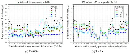
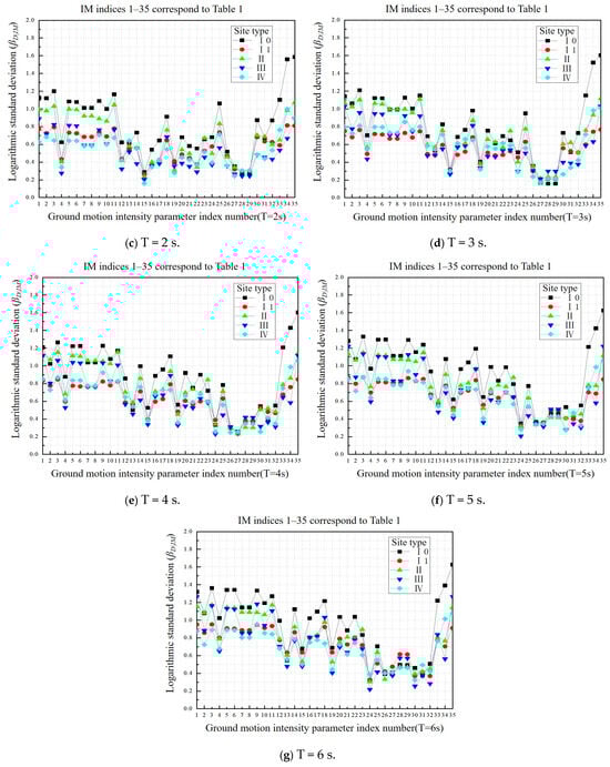
Figure 9. Comparison of efficiency (${\beta }_{D|IM}$) of ground motion intensity parameters under different site types.

The results of the efficiency analysis showed that:

(1) For structures with a short period of T = 0.5 s, ground motion intensity parameters show good efficiency when the site type is class III. However, Sa_avg, PGV, PSV, VSI, and I_H demonstrate the highest efficiency and are least impacted by variations in site conditions. Parameters related to velocity are less affected by changes in site type, whereas parameters associated with acceleration and displacement exhibit larger variations in efficiency with changes in site type.

(2) In the mid-period range (T = 1–3 s), the performance of Sd_avg, EPD, and DSI improves as the period increases, while the impact of site type variations on their efficiency diminishes. In contrast, the efficiency of Sa_avg and EPV declines with the increase in structural period, and they demonstrate higher sensitivity to variations in site types. The performance of V_rs, on the other hand, gradually reaches a stable value of around 0.3 as the period increases and is minimally affected by site type variations.

(3) The efficiency of PGD is the best for long-period structures (T = 4–6 s) and is almost not affected by changes in structural period or site type. On the other hand, the efficiency of V_rs decreases as the period increases.

(4) Throughout the entire structural period, there is a decreasing trend in the intensity parameters associated with acceleration as the structural period increases. The efficiency of intensity parameters associated with velocity initially increases and then declines. On the other hand, the efficiency of intensity parameters related to displacement improves over time. The intensity parameters that exhibit good efficiency are less influenced by variations in site type, whereas those with poor efficiency demonstrate higher variability.

(5) Time-related parameters (FR₁, FR₂, T_D) exhibit significantly weaker correlations with the maximum structural response, fundamentally due to an inherent mismatch between their physical nature and the mechanisms of structural nonlinear response. As dimensionless frequency indicator parameters, FR₁ and FR₂ only reflect the spectral characteristics of the ground motion input and cannot directly characterize the actual deformation and energy dissipation of the structure in its nonlinear state. Meanwhile, T_D, as a macro-duration indicator, fails to distinguish the contribution of cyclic loading with different amplitudes to cumulative damage, overlooking the nonlinear threshold effect. These parameters focus on describing the temporal or spectral characteristics of the ground motion, rather than directly capturing the mechanical mechanisms driving the structural response, resulting in their weaker statistical correlation.

3.6. Statistical Results of Applicability and Analysis

Applicability refers to the generalizability of the intensity measure across different types of structures and site conditions. An ideal IM should have broad applicability and be suitable for structural analysis under various seismic contexts. When the regression model of earthquake demand means is introduced into the probabilistic earthquake demand model, the following equation is obtained:

$$P[D\ge d|IM]=\mathsf{\Phi }\left({\displaystyle \frac{\mathrm{In}(IM)-[\mathrm{In}(d)-\mathrm{In}(a)]/b}{{\beta }_{D|IM}/b}}\right)$$

(14)

where $\zeta ={\beta }_{D|IM}/b$ represents the corrected logarithmic standard deviation. Padgett used the term “applicability” to describe $\zeta$. A smaller value of the applicability index indicates a higher level of applicability for the ground motion intensity measures.

The comparison results of the applicability of different structural periods under four site types are presented in Figure 10a–g.

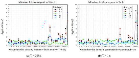
Figure 10. Comparison of applicability ($\zeta$) of ground motion intensity parameters under different site types.

The results of the applicability analysis show that:

(1) For short-period structures (T = 0.5 s), PGA, PSA, EPA, A_rs, and I_C have good applicability in class IV sites and have less influence from the change in site type in terms of displacement-related intensity parameters and FR₁, FR₂, and T_D. In class I sites, Sa_avg, PGV, PSV, VSI, I_F, and I_H have good applicability and are less influenced by the change in site type. However, CAI, D_rs, D_rms, I_d, FR₂, and T_D are more sensitive to changes in site type.

(2) For the mid-period range (T = 1–3 s), PGV, Sv_avg, V_rs, PSD, Sd_avg, EPD, DSI, and D_rs are the most suitable parameters, except for class II sites. The applicability of CAI, D_rs, D_rms, and I_d improves with increasing structure period, while being significantly affected by changes in site type, leading to decreased adaptability variability.

(3) The intensity parameters PGD, PSD, Sd_avg, D_rs, DSI, EPD, D_rms, and I_d are better suited for long-period structures (T = 4–6 s) that are related to displacement. I_a, Sv_avg, and V_rs also show relatively good applicability, but their suitability is lower for class II sites.

3.7. Statistical Results of Completeness and Analysis

Completeness is a crucial metric for assessing the accuracy of a probabilistic earthquake demand model, as it determines whether the intensity measure can comprehensively reflect the structural performance during an earthquake. A complete IM should encompass all the important seismic characteristics that influence the structural response, ensuring that the model accurately captures the full impact of seismic events on the structure.

The completeness is operationally defined as the statistical independence of the seismic demand residuals with respect to the moment magnitude (Mw), given the intensity measure (IM). The independence was assessed through linear regression analysis. A significance level of α = 0.05 was utilized; p > 0.5 means “complete”.

Taking the Arias intensity (I_A) as an example, the completeness between the ground motion intensity parameters and the structural response under the I₀ site type at T = 0.5 s is illustrated, as shown in Figure 11.

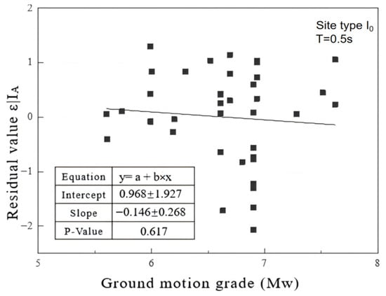
Figure 11. Completeness evaluation of Arias intensity and magnitude.

Figure 12a–g show the completeness of each intensity parameter and magnitude under different structural periods and site types.

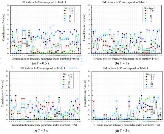
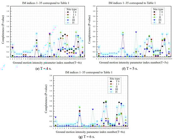
Figure 12. Comparison of completeness (p-value) of ground motion intensity parameters under different site types.

Based on the comparative analysis of the completeness results presented above, it can be concluded that changes in site conditions have a significant impact on intensity parameters, particularly for short- and medium-period structures. The completeness of seismic motion input varies under different site conditions, emphasizing the need for further research on the completeness of intensity parameters. However, for long-period structures, intensity parameters related to displacement demonstrate better completeness as the structural period increases, while those related to acceleration and velocity exhibit lower completeness.

Class IV soft soil sites exhibit significant site effects under seismic action, characterized by generally longer predominant periods, pronounced amplification of seismic waves, and a propensity for nonlinear dynamic response. These characteristics necessitate a distinct strategy for selecting ground motion intensity measures (IMs) compared to site classes I–III. To accurately capture the long-period vibration characteristics and cumulative damage mechanisms of soft soil sites, priority should be given to parameters sensitive to low-frequency components, such as Peak Spectral Displacement (PSD), Peak Ground Displacement (PGD), and Cumulative Absolute Velocity (CAV). These parameters can more effectively characterize the deformation evolution process and energy absorption behavior of soft soils under strong earthquake shaking, thereby improving the accuracy of seismic response predictions.

4. Statistical Analysis of Structural Response and Ground Motion Intensity Parameters Under Different Hysteretic Models

4.1. Selection of Ground Motion Acceleration Records

Another 50 ground motion records are selected from 178 ground motion records according to the following principles:

• The ground motion magnitude Mw > 5.5 and PGA > 0.1 g ensure that the selected ground motion record had a sufficient level of intensity.
• The distance from the epicenter, denoted as R, falls within the range of 0 km to 100 km (0 km< R< 100 km). This range ensures that the ground motion records selected for analysis include seismic information from both near-field and far-field locations and encompass all types of sites.

Figure 13 shows the acceleration response spectrum curve of the selected ground motion records in the logarithmic coordinate system, considering a damping ratio of 5%. Further information regarding the selected ground motion records can be found in Table A8 and Table A9 in Appendix A.

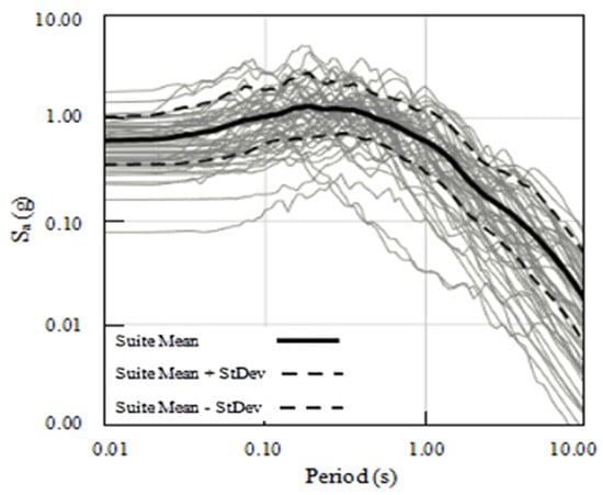
Figure 13. Ground motion acceleration response spectrum selected in this section.

4.2. Statistical Analysis of Ground Motion Intensity Parameters Under Different Hysteretic Models

In the presence of earthquake excitation, a nonlinear time-history analysis is performed on different nonlinear SDOF structures with two different hysteresis models. The maximum displacement of the structure is considered as the structural demand parameter to analyze the correlation, efficiency, applicability, and completeness of ground motion intensity parameters. The evaluation results are compared between the two different hysteresis models. Model 1 is a bilinear hysteresis model (Figure 14), and Model 2 is a Clough stiffness-degrading bilinear hysteretic model.

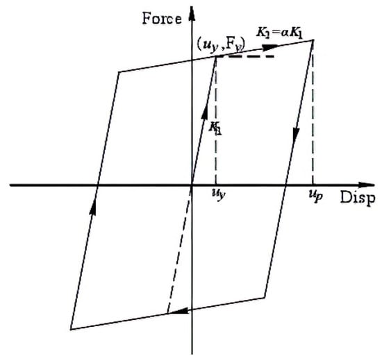
Figure 14. Bilinear hysteretic model.

4.3. Comparative Analysis of Correlation of Ground Motion Intensity Parameters Under Two Hysteretic Models

The logarithmic linear regression analysis was performed on the structural demand parameter (DM) and the ground motion intensity parameter (IM) using the maximum displacement of the structure as the requirement parameter. The correlation between the ground motion intensity parameter and different hysteresis models was evaluated based on the regression results. The calculation results of R² are shown in Table 4 and Figure 15a–g, where a higher R² value indicates a stronger correlation.

Table 4. Correlation of ground motion intensity parameters under two hysteretic models R².

Intensity Parameters	T = 0.5 s		T = 1 s		T = 2 s		T = 3 s		T = 4 s		T = 5 s		T = 6 s
	1	2	1	2	1	2	1	2	1	2	1	2	1	2
PGA	0.36	0.37	0.17	0.2	0.15	0.19	0.13	0.16	0.13	0.12	0.14	0.11	0.08	0.1
CAV	0.18	0.17	0.21	0.19	0.28	0.28	0.33	0.34	0.36	0.36	0.35	0.35	0.36	0.38
PSA	0.18	0.22	0.09	0.1	0.09	0.13	0.1	0.12	0.08	0.08	0.09	0.09	0.07	0.09
Saavg	0.82	0.8	0.84	0.87	0.84	0.85	0.77	0.76	0.71	0.69	0.69	0.66	0.59	0.59
EPA	0.39	0.44	0.2	0.21	0.17	0.2	0.17	0.18	0.15	0.14	0.16	0.14	0.12	0.13
ASI	0.41	0.46	0.22	0.22	0.19	0.21	0.18	0.19	0.16	0.15	0.17	0.15	0.13	0.14
IA	0.4	0.4	0.35	0.35	0.38	0.4	0.38	0.4	0.38	0.37	0.37	0.36	0.33	0.35
Ars	0.4	0.4	0.35	0.35	0.38	0.4	0.38	0.4	0.38	0.37	0.37	0.36	0.33	0.35
Arms	0.41	0.44	0.35	0.36	0.3	0.35	0.28	0.28	0.25	0.24	0.25	0.23	0.18	0.2
IC	0.46	0.48	0.4	0.41	0.4	0.44	0.39	0.41	0.38	0.37	0.37	0.35	0.31	0.34
Ia	0.25	0.25	0.11	0.13	0.12	0.15	0.12	0.14	0.13	0.12	0.13	0.11	0.1	0.11
PGV	0.84	0.8	0.81	0.82	0.79	0.8	0.74	0.74	0.71	0.68	0.69	0.66	0.59	0.59
CAD	0.38	0.34	0.53	0.5	0.64	0.62	0.71	0.69	0.73	0.73	0.73	0.72	0.74	0.72
PSV	0.81	0.77	0.82	0.82	0.77	0.76	0.67	0.65	0.61	0.58	0.59	0.56	0.52	0.51
Svavg	0.68	0.63	0.86	0.88	0.94	0.95	0.94	0.93	0.89	0.89	0.87	0.86	0.8	0.79
EPV	0.73	0.69	0.94	0.98	0.92	0.88	0.74	0.71	0.66	0.65	0.64	0.61	0.53	0.52
VSI	0.84	0.82	0.93	0.95	0.87	0.84	0.71	0.69	0.64	0.62	0.62	0.59	0.51	0.51
IA,M	0.52	0.53	0.57	0.53	0.48	0.49	0.44	0.4	0.34	0.36	0.32	0.34	0.3	0.32
Vrs	0.64	0.59	0.8	0.79	0.88	0.87	0.89	0.88	0.88	0.88	0.87	0.86	0.83	0.82
Vrms	0.65	0.63	0.79	0.8	0.78	0.8	0.76	0.75	0.72	0.72	0.72	0.7	0.64	0.64
IF	0.79	0.74	0.77	0.78	0.8	0.79	0.76	0.77	0.76	0.72	0.73	0.71	0.65	0.65
IH	0.81	0.78	0.93	0.95	0.91	0.89	0.76	0.73	0.69	0.67	0.66	0.63	0.55	0.55
Iv	0.64	0.58	0.63	0.63	0.69	0.67	0.68	0.69	0.69	0.66	0.66	0.65	0.61	0.61
PGD	0.43	0.37	0.59	0.61	0.74	0.75	0.84	0.86	0.92	0.93	0.93	0.95	0.94	0.94
CAI	0.21	0.17	0.34	0.31	0.49	0.48	0.63	0.64	0.71	0.73	0.74	0.75	0.79	0.79
PSD	0.48	0.43	0.66	0.67	0.8	0.81	0.9	0.9	0.92	0.93	0.93	0.93	0.92	0.91
Sdavg	0.56	0.5	0.76	0.78	0.9	0.91	0.96	0.96	0.94	0.96	0.94	0.93	0.89	0.88
EPD	0.52	0.48	0.74	0.74	0.88	0.92	0.94	0.94	0.88	0.88	0.85	0.83	0.78	0.77
DSI	0.52	0.47	0.74	0.74	0.88	0.92	0.94	0.95	0.88	0.88	0.85	0.83	0.78	0.77
Drs	0.3	0.25	0.46	0.44	0.62	0.63	0.77	0.78	0.84	0.87	0.87	0.89	0.91	0.91
Drms	0.37	0.32	0.53	0.52	0.65	0.68	0.79	0.8	0.84	0.87	0.88	0.89	0.89	0.89
Id	0.34	0.28	0.49	0.49	0.65	0.65	0.76	0.78	0.84	0.86	0.86	0.88	0.88	0.89
FR1	0.3	0.26	0.51	0.48	0.53	0.47	0.51	0.47	0.48	0.48	0.45	0.46	0.44	0.42
FR2	−0.02	−0.02	0.04	0.04	0.14	0.15	0.26	0.28	0.35	0.4	0.39	0.43	0.48	0.49
TD	−0.01	−0.01	−0.02	−0.02	−0.01	−0.01	0.01	0.01	0.03	0.04	0.03	0.04	0.06	0.06

1: hysteretic model 1; 2: hysteretic model 2.

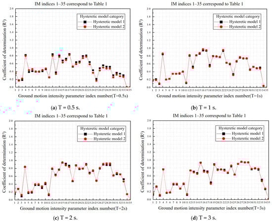
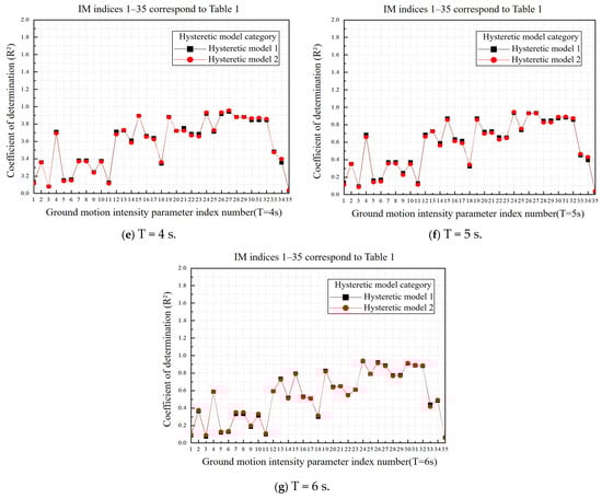
Figure 15. Correlation of ground motion intensity parameters under two hysteresis models.

By comparing Table 4 and Figure 15a–g, at T = 0.5 s, the optimal IMs are ranked as follows: VSI, PGV, Sa_avg, PSV, and I_H, with R² values all exceeding 0.8. For the T = 1–3 s range, the parameters that show relatively good correlation are: Sv_avg, EPV, VSI, V_rs, PSD, Sd_avg, EPD, and DSI. For the T = 4–6 s, PGD, PSD, Sd_avg, EPD, DSI, D_rs, D_rms, and I_d exhibit significant correlations. Particularly, in the medium- to long-period range, PSD, Sd_avg, EPD, and DSI exhibit stronger correlations. Under both bilinear and Clough stiffness-degrading bilinear hysteretic models, the correlation between ground motion intensity measures (IMs) and the maximum structural seismic response remains generally consistent, with no significant differences observed. This is because the structural response is primarily governed by the skeleton curve and the overall energy dissipation capacity, which are fundamentally similar in both models. In the short-period range, displacement-type parameters exhibit a slightly higher correlation under the bilinear model. This can be attributed to the stiffness degradation effect in the Clough model, which increases the dispersion of responses and weakens the strength of statistical correlation. For engineering applications, the simpler bilinear model can be used for preliminary screening of IMs in medium- to long-period structures or for trend analysis; for short-period structures or when precise consideration of cumulative damage is required, the Clough model is recommended to account for the effects of stiffness degradation.

4.4. Comparative Analysis of the Efficiency of Ground Motion Intensity Parameters Under Two Hysteretic Models

The efficiency of the ground motion intensity measures (IMs) under two different hysteresis models is shown in Table 5 and Figure 16a–g. A smaller efficiency index indicates a better efficiency of the IM.

Table 5. Efficiency of ground motion intensity parameters under two hysteretic models ${\beta }_{D|IM}$.

Intensity Parameter	T = 0.5 s		T = 1 s		T = 2 s		T = 3 s		T = 4 s		T = 5 s		T = 6 s
	1	2	1	2	1	2	1	2	1	2	1	l2	1	2
PGA	0.57	0.64	0.82	0.86	0.88	0.88	0.99	1.00	1.08	1.10	1.12	1.15	1.14	1.17
CAV	0.65	0.74	0.80	0.87	0.81	0.83	0.87	0.89	0.92	0.94	0.97	0.98	0.95	0.97
PSA	0.65	0.72	0.86	0.91	0.91	0.91	1.01	1.02	1.11	1.12	1.15	1.16	1.15	1.18
Saavg	0.30	0.36	0.36	0.35	0.38	0.38	0.51	0.53	0.62	0.65	0.67	0.71	0.77	0.79
EPA	0.56	0.61	0.81	0.86	0.87	0.88	0.97	0.99	1.06	1.08	1.11	1.13	1.12	1.15
ASI	0.55	0.59	0.80	0.85	0.86	0.87	0.97	0.98	1.06	1.08	1.10	1.12	1.12	1.15
IA	0.55	0.63	0.73	0.78	0.75	0.76	0.84	0.84	0.91	0.93	0.96	0.98	0.98	0.99
Ars	0.55	0.63	0.73	0.78	0.75	0.76	0.84	0.85	0.91	0.93	0.96	0.98	0.98	0.99
Arms	0.55	0.61	0.73	0.77	0.80	0.79	0.91	0.92	1.00	1.02	1.05	1.07	1.08	1.10
IC	0.52	0.59	0.70	0.74	0.74	0.73	0.83	0.84	0.91	0.93	0.96	0.98	0.99	1.01
Ia	0.62	0.70	0.85	0.90	0.90	0.90	1.00	1.01	1.08	1.10	1.13	1.15	1.13	1.16
PGV	0.29	0.36	0.40	0.41	0.44	0.44	0.55	0.56	0.62	0.66	0.67	0.71	0.76	0.79
CAD	0.56	0.66	0.62	0.68	0.57	0.60	0.58	0.61	0.60	0.61	0.63	0.64	0.61	0.65
PSV	0.31	0.39	0.39	0.41	0.46	0.48	0.61	0.64	0.72	0.75	0.77	0.80	0.83	0.86
Svavg	0.40	0.49	0.34	0.34	0.22	0.21	0.27	0.29	0.37	0.38	0.43	0.46	0.54	0.57
EPV	0.37	0.45	0.22	0.15	0.27	0.34	0.55	0.59	0.67	0.69	0.73	0.76	0.82	0.85
VSI	0.28	0.34	0.23	0.22	0.35	0.39	0.57	0.61	0.69	0.72	0.75	0.78	0.83	0.87
IA,M	0.49	0.56	0.59	0.66	0.69	0.70	0.80	0.85	0.94	0.93	1.00	0.99	1.00	1.02
Vrs	0.43	0.52	0.40	0.44	0.33	0.35	0.35	0.38	0.40	0.41	0.43	0.46	0.49	0.53
Vrms	0.42	0.50	0.42	0.44	0.45	0.44	0.52	0.55	0.61	0.62	0.64	0.67	0.71	0.75
IF	0.32	0.41	0.43	0.45	0.43	0.45	0.52	0.52	0.57	0.61	0.63	0.66	0.71	0.73
IH	0.31	0.38	0.24	0.21	0.29	0.32	0.52	0.56	0.64	0.67	0.71	0.74	0.80	0.83
Iv	0.43	0.52	0.55	0.59	0.53	0.56	0.61	0.61	0.64	0.68	0.71	0.72	0.75	0.77
PGD	0.54	0.64	0.58	0.61	0.49	0.49	0.43	0.41	0.33	0.30	0.31	0.28	0.30	0.30
CAI	0.63	0.74	0.73	0.80	0.68	0.70	0.65	0.66	0.62	0.61	0.62	0.60	0.55	0.56
PSD	0.51	0.61	0.53	0.55	0.43	0.42	0.33	0.34	0.34	0.30	0.31	0.32	0.33	0.37
Sdavg	0.47	0.57	0.44	0.46	0.31	0.29	0.22	0.22	0.28	0.24	0.31	0.32	0.40	0.42
EPD	0.49	0.59	0.46	0.49	0.33	0.27	0.26	0.26	0.40	0.40	0.47	0.51	0.56	0.60
DSI	0.49	0.59	0.46	0.49	0.33	0.27	0.26	0.26	0.39	0.40	0.47	0.51	0.56	0.60
Drs	0.59	0.70	0.67	0.72	0.59	0.60	0.51	0.51	0.46	0.43	0.43	0.40	0.36	0.36
Drms	0.57	0.67	0.62	0.67	0.56	0.55	0.49	0.49	0.45	0.42	0.41	0.40	0.40	0.40
Id	0.58	0.69	0.65	0.69	0.57	0.58	0.53	0.51	0.46	0.44	0.46	0.43	0.41	0.41
FR1	0.59	0.70	0.63	0.70	0.66	0.71	0.75	0.80	0.83	0.85	0.90	0.89	0.89	0.94
FR2	0.72	0.82	0.89	0.94	0.88	0.90	0.92	0.93	0.93	0.91	0.94	0.92	0.86	0.88
TD	0.72	0.81	0.91	0.98	0.96	0.98	1.06	1.09	1.14	1.15	1.19	1.19	1.15	1.20

1: hysteretic model 1; 2: hysteretic model 2.

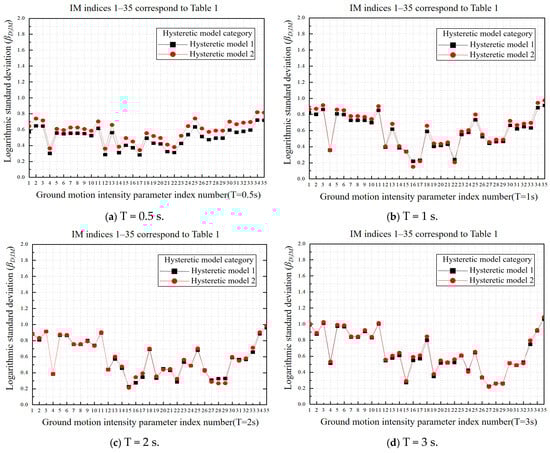
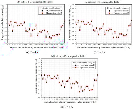
Figure 16. Efficiency of ground motion intensity parameters under two hysteretic models.

The evaluation results of IM efficiency are consistent for the two hysteresis models. The efficiency results are generally similar for the entire structural period (T = 0.5–6 s) under different hysteresis models. However, at T = 0.5 s, the efficiency of the bilinear hysteresis model is better than that of the Clough-degraded bilinear hysteresis model. At the same time, IMs with good correlation also have good efficiency.

4.5. Comparative Analysis on the Applicability of Ground Motion Intensity Parameters Under Two Hysteretic Models

The applicability index is a comprehensive evaluation indicator that combines efficiency indicators with slopes obtained from regression analysis in order to achieve a balance. The applicability calculation results $\zeta$ of the ground motion intensity measures (IMs) under two different hysteretic models are shown in Table 6 and Figure 17a–g. The smaller the applicability index, the higher the applicability of IMs.

Table 6. Applicability of ground motion intensity parameters under two hysteretic models $\zeta$.

Intensity Parameter	T = 0.5 s		T = 1 s		T = 2 s		T = 3 s		T = 4 s		T = 5 s		T = 6 s
	1	2	1	2	1	2	1	2	1	2	1	l2	1	2
PGA	0.80	0.78	1.27	1.17	1.37	1.20	1.46	1.35	1.47	1.56	1.44	1.58	1.81	1.69
CAV	1.31	1.35	1.18	1.26	0.98	1.00	0.89	0.87	0.83	0.83	0.84	0.85	0.83	0.80
PSA	1.07	0.96	1.55	1.44	1.55	1.29	1.45	1.34	1.61	1.61	1.50	1.57	1.71	1.53
Saavg	0.31	0.34	0.29	0.27	0.30	0.29	0.37	0.38	0.43	0.45	0.45	0.48	0.56	0.56
EPA	0.74	0.67	1.14	1.13	1.24	1.15	1.26	1.22	1.32	1.38	1.28	1.38	1.51	1.44
ASI	0.71	0.64	1.10	1.09	1.20	1.12	1.22	1.20	1.29	1.35	1.25	1.35	1.47	1.41
IA	1.24	1.23	1.37	1.37	1.29	1.24	1.28	1.23	1.29	1.31	1.30	1.35	1.43	1.36
Ars	0.62	0.61	0.69	0.69	0.65	0.62	0.64	0.62	0.64	0.66	0.65	0.68	0.71	0.68
Arms	0.73	0.68	0.81	0.79	0.91	0.82	0.96	0.94	1.03	1.05	1.03	1.09	1.22	1.17
IC	0.82	0.79	0.92	0.91	0.92	0.86	0.93	0.91	0.97	0.99	0.98	1.02	1.11	1.05
Ia	1.05	1.06	1.66	1.55	1.58	1.44	1.61	1.47	1.53	1.62	1.53	1.63	1.76	1.65
PGV	0.33	0.38	0.37	0.35	0.40	0.38	0.46	0.45	0.48	0.52	0.51	0.54	0.63	0.63
CAD	1.17	1.27	0.86	0.92	0.69	0.72	0.59	0.62	0.57	0.56	0.57	0.57	0.55	0.57
PSV	0.36	0.40	0.35	0.35	0.41	0.42	0.52	0.54	0.59	0.63	0.62	0.65	0.71	0.73
Svavg	0.61	0.68	0.36	0.33	0.22	0.20	0.23	0.25	0.31	0.31	0.34	0.36	0.45	0.46
EPV	0.57	0.62	0.23	0.15	0.28	0.35	0.56	0.60	0.66	0.67	0.70	0.74	0.87	0.88
VSI	0.34	0.37	0.21	0.19	0.31	0.35	0.50	0.54	0.59	0.61	0.63	0.66	0.77	0.78
IA,M	1.30	1.28	1.18	1.27	1.43	1.40	1.53	1.65	1.87	1.79	1.95	1.87	2.06	1.98
Vrs	0.62	0.69	0.41	0.42	0.31	0.32	0.29	0.31	0.30	0.31	0.31	0.34	0.37	0.39
Vrms	0.67	0.71	0.48	0.46	0.49	0.46	0.51	0.53	0.57	0.57	0.57	0.60	0.68	0.69
IF	0.38	0.44	0.41	0.40	0.38	0.39	0.42	0.41	0.42	0.46	0.46	0.48	0.55	0.55
IH	0.39	0.43	0.22	0.18	0.25	0.28	0.45	0.48	0.54	0.56	0.58	0.61	0.72	0.73
Iv	0.39	0.44	0.40	0.40	0.35	0.37	0.36	0.36	0.35	0.38	0.38	0.39	0.42	0.42
PGD	1.25	1.43	0.92	0.89	0.66	0.64	0.48	0.44	0.34	0.30	0.30	0.26	0.29	0.27
CAI	2.55	2.92	1.87	1.97	1.38	1.40	1.03	1.02	0.87	0.83	0.81	0.78	0.70	0.69
PSD	1.07	1.20	0.75	0.73	0.53	0.50	0.34	0.34	0.32	0.28	0.28	0.29	0.30	0.33
Sdavg	0.90	1.00	0.57	0.55	0.35	0.31	0.22	0.21	0.26	0.22	0.27	0.28	0.36	0.37
EPD	0.98	1.07	0.62	0.60	0.38	0.30	0.26	0.25	0.38	0.38	0.44	0.47	0.55	0.57
DSI	0.98	1.08	0.62	0.61	0.38	0.30	0.26	0.25	0.38	0.38	0.44	0.47	0.55	0.57
Drs	1.85	2.10	1.35	1.39	0.98	0.96	0.69	0.66	0.54	0.49	0.48	0.44	0.40	0.38
Drms	1.67	1.85	1.22	1.23	0.94	0.88	0.66	0.65	0.55	0.50	0.47	0.45	0.46	0.45
Id	1.57	1.81	1.18	1.16	0.85	0.85	0.66	0.61	0.50	0.47	0.48	0.44	0.43	0.41
FR1	0.87	0.96	0.58	0.61	0.56	0.62	0.58	0.62	0.61	0.61	0.65	0.63	0.65	0.69
FR2	5.01	7.98	2.73	2.64	1.56	1.54	1.11	1.06	0.90	0.82	0.83	0.77	0.70	0.68
TD	5.96	6.90	5.95	6.13	6.30	8.45	3.73	3.86	2.98	2.81	2.92	2.78	2.32	2.39

1: hysteretic model 1; 2: hysteretic model 2.

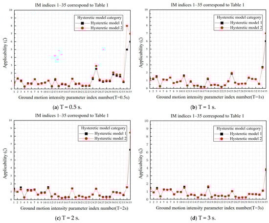
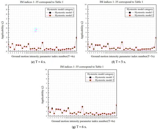
Figure 17. Applicability of ground motion intensity parameters under two hysteretic models.

According to Table 6 and Figure 17a–g, it can be observed that the suitability analysis results of the two hysteresis models for IMs remain consistent and are not sensitive to changes in the hysteresis model. For short-period structures (T = 0.5 s), most of the IMs related to acceleration and velocity, except for CAV, PSA, I_A, I_a, CAD, and I_A,M, have values less than 1, indicating good suitability. As the structural period increases, the suitability of IMs related to acceleration gradually deteriorates, while the suitability of IMs related to velocity displacement improves, particularly for CAI. However, the suitability of IMs related to strong-motion duration (T_D) is relatively poor.

4.6. Comparative Analysis of the Completeness of Ground Motion Intensity Parameters Under Two Hysteretic Models

The completeness calculations for the ground motion intensity parameters under two different hysteretic models are presented in Table 7 and depicted in Figure 18a–g. The larger the p-value of the completeness index, the greater the completeness of the ground motion intensity measures.

Table 7. Completeness p-value of ground motion intensity parameters under two hysteretic models.

Intensity Parameter	T = 0.5 s		T = 1 s		T = 2 s		T = 3 s		T = 4 s		T = 5 s		T = 6 s
	1	2	1	2	1	2	1	2	1	2	1	l2	1	2
PGA	0.02	0.03	0.01	0.02	0.00	0.00	0.00	0.00	0.00	0.00	0.00	0.00	0.00	0.00
CAV	0.91	0.80	0.82	0.98	0.56	0.62	0.15	0.12	0.07	0.08	0.06	0.05	0.02	0.02
PSA	0.08	0.12	0.02	0.05	0.00	0.00	0.00	0.00	0.00	0.00	0.00	0.00	0.00	0.00
Saavg	0.48	0.32	0.73	0.62	0.06	0.10	0.00	0.00	0.00	0.00	0.00	0.00	0.00	0.00
EPA	0.06	0.10	0.02	0.05	0.00	0.00	0.00	0.00	0.00	0.00	0.00	0.00	0.00	0.00
ASI	0.07	0.10	0.02	0.05	0.00	0.00	0.00	0.00	0.00	0.00	0.00	0.00	0.00	0.00
IA	0.99	0.82	0.47	0.72	0.15	0.21	0.01	0.01	0.00	0.00	0.00	0.00	0.00	0.00
Ars	0.99	0.82	0.47	0.72	0.15	0.21	0.01	0.01	0.00	0.00	0.00	0.00	0.00	0.00
Arms	0.06	0.09	0.01	0.04	0.00	0.00	0.00	0.00	0.00	0.00	0.00	0.00	0.00	0.00
IC	0.63	0.84	0.23	0.42	0.05	0.07	0.00	0.00	0.00	0.00	0.00	0.00	0.00	0.00
Ia	0.13	0.20	0.04	0.08	0.01	0.01	0.00	0.00	0.00	0.00	0.00	0.00	0.00	0.00
PGV	0.29	0.22	0.84	0.60	0.12	0.18	0.00	0.00	0.00	0.00	0.00	0.00	0.00	0.00
CAD	0.17	0.18	0.10	0.06	0.16	0.15	0.78	0.99	0.76	0.88	0.74	0.60	0.31	0.26
PSV	0.33	0.25	0.93	0.53	0.14	0.21	0.00	0.00	0.00	0.00	0.00	0.00	0.00	0.00
Svavg	0.12	0.12	0.05	0.00	0.25	0.08	0.01	0.00	0.00	0.00	0.00	0.00	0.00	0.00
EPV	0.85	0.95	0.17	0.99	0.00	0.01	0.00	0.00	0.00	0.00	0.00	0.00	0.00	0.00
VSI	0.98	0.70	0.16	0.81	0.00	0.01	0.00	0.00	0.00	0.00	0.00	0.00	0.00	0.00
IA,M	0.60	0.80	0.24	0.44	0.04	0.05	0.00	0.00	0.00	0.00	0.00	0.00	0.00	0.00
Vrs	0.03	0.03	0.01	0.00	0.03	0.02	0.82	0.54	0.18	0.25	0.16	0.10	0.02	0.01
Vrms	0.82	0.65	0.76	0.72	0.11	0.16	0.00	0.00	0.00	0.00	0.00	0.00	0.00	0.00
IF	0.02	0.02	0.25	0.07	0.99	0.85	0.05	0.03	0.01	0.01	0.01	0.00	0.00	0.00
IH	0.76	0.56	0.47	0.55	0.01	0.02	0.00	0.00	0.00	0.00	0.00	0.00	0.00	0.00
Iv	0.04	0.05	0.25	0.10	0.67	0.62	0.24	0.18	0.07	0.08	0.06	0.04	0.01	0.01
PGD	0.14	0.18	0.08	0.02	0.08	0.04	0.49	0.57	0.77	0.46	0.68	0.85	0.30	0.24
CAI	0.39	0.46	0.24	0.17	0.17	0.15	0.31	0.38	0.34	0.22	0.26	0.28	0.43	0.46
PSD	0.11	0.12	0.04	0.01	0.04	0.01	0.37	0.58	0.85	0.83	0.90	0.62	0.12	0.10
Sdavg	0.12	0.13	0.04	0.00	0.03	0.00	0.77	0.41	0.06	0.08	0.05	0.02	0.00	0.00
EPD	0.30	0.28	0.16	0.04	0.24	0.03	0.14	0.04	0.01	0.02	0.02	0.01	0.00	0.00
DSI	0.29	0.28	0.16	0.04	0.23	0.03	0.14	0.05	0.01	0.02	0.02	0.01	0.00	0.00
Drs	0.19	0.24	0.09	0.05	0.05	0.03	0.11	0.13	0.11	0.04	0.05	0.05	0.18	0.18
Drms	0.30	0.31	0.21	0.09	0.30	0.15	0.83	0.99	0.72	0.98	0.84	0.66	0.19	0.16
Id	0.19	0.26	0.12	0.04	0.08	0.06	0.36	0.39	0.43	0.26	0.39	0.43	0.97	1.00
FR1	0.99	0.95	0.96	0.72	0.45	0.45	0.04	0.02	0.01	0.01	0.01	0.00	0.00	0.00
FR2	0.10	0.09	0.20	0.35	0.21	0.27	0.08	0.07	0.06	0.10	0.08	0.07	0.04	0.04
TD	0.02	0.03	0.02	0.03	0.01	0.01	0.00	0.00	0.00	0.00	0.00	0.00	0.00	0.00

1: hysteretic model 1; 2: hysteretic model 2.

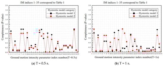
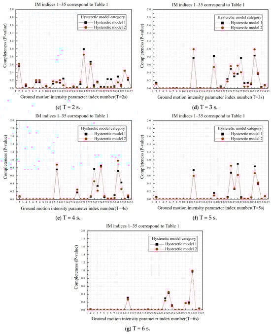
Figure 18. Completeness of ground motion intensity parameters under two hysteretic models.

Based on the analysis of Table 7 and Figure 18a–g, it can be concluded that for short-period structures (T = 0.5 s), the complete assessment of CAV, Sa_avg, I_A, A_rs, VSI, V_rms, and I_H is better under the bilinear hysteretic model than the Clough degradation bilinear hysteretic model. When T = 1 s, EPV and VSI are greatly influenced by the change in the hysteretic model, which leads to inconsistent evaluation results under different hysteretic models. However, this discrepancy gradually disappears with the increase in the structural period.

Under both the Clough stiffness-degrading bilinear hysteretic model and the bilinear hysteretic model as constitutive relationships, the evaluation results of various ground motion intensity measures (IMs) in terms of correlation, efficiency, applicability, and completeness show no significant differences attributable to the hysteretic model used. This indicates that the optimal IMs selected in this study exhibit low sensitivity to the specific manifestations of structural nonlinear behavior, such as stiffness degradation. This robustness can be explained by the equivalent modal damping ratio theory proposed in reference [51]: when the spectral characteristics of an intensity measure match the equivalent modal damping ratio of the structure in its nonlinear state, its dependence on the specific form of the hysteretic model is significantly reduced. Consequently, even under the fundamentally different nonlinear constitutive assumptions of the bilinear (no degradation) and Clough degrading (considering stiffness degradation) models, the selected optimal intensity measures maintain stable evaluation performance.

5. Conclusions

In the performance-based earthquake engineering framework, the selection of appropriate ground motion intensity measures (IMs) plays a crucial role in accurately assessing the seismic performance of structures based on probability. The optimal IMs should have a high correlation with the structural probabilistic seismic demand and should also be effective, applicable, and comprehensive. The present study investigates the relationship between the seismic response of nonlinear single-degree-of-freedom structures and IMs through extensive statistical analysis, mainly drawing the following conclusions:

• There exists a strong correlation between acceleration-type, velocity-type, and displacement-type intensity parameters. Among these parameters, the rank correlation coefficient between I_A and A_rs, EPD, and DSI is consistently 1, suggesting they can be considered as the same intensity parameter. Similarly, the rank correlation coefficients between EPA and ASI, EPV, VSI, and I_H are all above 0.99, suggesting they can also be considered as the same intensity parameter, given certain conditions.
• Through the evaluation based on correlation, efficiency, applicability, and completeness, it can be seen that the intensity parameters Sv_avg and Sd_avg are generally applicable to all different site types of seismic input or various structural period ranges. Meanwhile, acceleration-related intensity parameters, represented by PGA and Sa_avg, perform well in the short-period range; velocity-related intensity parameters, such as PGV, are more suitable for medium-period structures; and displacement-related intensity parameters, represented by PGD, are better suited for long-period structures. Furthermore, these intensity parameters, which exhibit good correlation with structural seismic demand across different periods, are relatively less affected by variations in seismic input due to different site types. Therefore, when selecting these intensity parameters, it is not necessary to consider the influence of differing seismic site types.
• This study demonstrates that under the selected bilinear hysteresis model and the Clough stiffness-degrading bilinear hysteretic model, the assessment results for the correlation, efficiency, applicability, and completeness of ground motion intensity parameters remain consistent, indicating that the selected IMs are robust for these two hysteresis models.

References

- Moehle, J.P.; Deierlein, G.G. A framework methodology for performance-based earthquake engineering. In Proceedings of the 13th World Conference on Earthquake Engineering, Vancouver, BC, Canada, 1–6 August 2004. [Google Scholar]
- Field, E.H. Some systemic risks to progress on seismic hazard assessment. Seismol. Soc. Am. 2022, 93, 513–551. [Google Scholar] [CrossRef]
- Shome, N. Probabilistic Seismic Demand Analysis of Nonlinear Structures. Ph.D. Thesis, Stanford University, Stanford, CA, USA, 1999. [Google Scholar]
- Asgarian, B.; Sadrinezhad, A.; Alanjari, P. Seismic performance evaluation of steel moment resisting frames through incremental dynamic analysis. J. Constr. Steel Res. 2010, 66, 178–190. [Google Scholar] [CrossRef]
- Bazzurro, P. Probabilistic Seismic Demand Analysis. Ph.D. Thesis, Stanford University, Stanford, CA, USA, 1998. [Google Scholar]
- Hu, S.; Liu, S.; Zeng, S.; Zhang, B.; Xu, Z. Investigating seismic performance of a novel self-centering shear link in EBF utilizing experimental and numerical simulation. J. Constr. Steel Res. 2025, 224, 109129. [Google Scholar]
- Pei, Q.; Zhong, Y.; Wang, B.; Qi, P.; Xue, Z.; Cui, D.; Ding, Y.; Cai, B. Performance of SRC unequal-depth beam-column irregular joint in NPP under progressive collapse. Structures 2024, 70, 107593. [Google Scholar]
- Pei, Q.; Wu, C.; Cheng, Z.; Ding, Y.; Guo, H. The Seismic Performance of New Self-Centering Beam-Column Joints of Conventional Island Main Buildings in Nuclear Power Plants. Materials 2022, 15, 1704. [Google Scholar] [PubMed]
- Liu, S.; Chen, S.; Zeng, S.; Zhang, B.; Hu, S. Seismic performance analysis of K-shaped EBF with an innovative crack-resistant composition beam. J. Build. Eng. 2025, 101, 111818. [Google Scholar]
- Wang, Y.; Hu, X.; Pei, Q.; Cui, X.; Qi, P.; Xue, Z. Improvement of mechanical behavior of cemented soil reinforced with waste sisal fibers: An optimal selection and modification research. Case Stud. Constr. Mater. 2024, 21, e03515. [Google Scholar] [CrossRef]
- Zucca, M.; Crespi, P.; Tropeano, G.; Simoncelli, M. On the Influence of Shallow Underaround Structures in the Evaluation of the Seismic Signals. Ing. Sismica 2021, 38, 23–35. [Google Scholar]
- Ministry of Housing Urban-Rural Development, PRC. Code for Seismic Design of Buildings; China Architecture & Building Press: Beijing, China, 2016. [Google Scholar]
- Hansen, R.J. Seismic Design for Nuclear Power Plants; MIT Press: Cambridge, MA, USA, 1970. [Google Scholar]
- Riddell, R.; Garcia, E.J. Hysteretic energy spectrum and damage control. Earthq. Eng. Struct. Dyn. 2001, 30, 1791–1816. [Google Scholar] [CrossRef]
- Park, Y.J.; Ang, A.H.; Wen, Y.K. Seismic damage analysis of reinforced concrete buildings. J. Struct. Eng. 1985, 111, 740–757. [Google Scholar] [CrossRef]
- Fajfar, P.; Vidic, T.; Fischinger, M. A measure of earthquake motion capacity to damage medium-period structures. Soil Dyn. Earthq. Eng. 1990, 9, 236–242. [Google Scholar] [CrossRef]
- Desai, R.; Tande, S. Estimate of peak relative velocity from conventional spectral velocity for response spectrum based force evaluation in damping devices. Structures 2018, 15, 378–387. [Google Scholar] [CrossRef]
- Mackie, K. Fragility-Based Seismic Decision Making for Highway Overpass Bridges. Ph.D. Thesis, University of California, Berkeley, CA, USA, 2004. [Google Scholar]
- Xie, L.L.; Zhang, X.Z. Accelerogram-based duration and engineering duration of ground motion. Earthq. Eng. Eng. Vib. 1988, 8, 31–38. [Google Scholar]
- Bolt, B.A. Duration of strong ground motion. In Proceedings of the 5th World Conference on Earthquake Engineering, Rome, Italy, 25–29 June 1973. [Google Scholar]
- Trifunac, M.D.; Brady, A.G. A study on the duration of strong duration earthquake ground motion. Bull. Seismol. Soc. Am. 1975, 65, 581–626. [Google Scholar]
- Jayaram, N.; Mollaioli, F.; Bazzurro, P.; Sortis, A.D.; Bruno, S. Prediction of structural response of reinforced concrete frames subjected to earthquake ground motions. In Proceedings of the 9th U.S. National and 10th Canadian Conference on Earthquake Engineering, Toronto, ON, Canada, 25–29 July 2010. [Google Scholar]
- Bianchini, M.; Diotallevi, P.P.; Baker, J.W. Prediction of inelastic structural response using an average of spectral accelerations. In Proceedings of the 10th International Conference on Structural Safety and Reliability, Osaka, Japan, 13–17 September 2009. [Google Scholar]
- Tajammolian, H.; Khoshnoudian, F.; Talaei, S.; Loghman, V. The effects of peak ground velocity of near-field ground motions on the seismic responses of base-isolated structures mounted on friction bearings. Earthq. Struct. 2014, 7, 1259–1282. [Google Scholar] [CrossRef]
- Giovenale, P.; Cornell, C.A.; Esteva, L. Comparing the adequacy of alternative ground motion intensity measures for the estimation of structural responses. Earthq. Eng. Struct. Dyn. 2004, 33, 951–979. [Google Scholar] [CrossRef]
- Luco, N.; Cornell, C.A. Effects of connection fractures on SMRF seismic drift demands. J. Struct. Eng. 2000, 126, 127–136. [Google Scholar] [CrossRef]
- Yakut, A.; Yilmaz, H. Correlation of deformation demands with ground motion intensity. J. Struct. Eng. 2008, 134, 1818–1828. [Google Scholar] [CrossRef]
- Kostinakis, K.G.; Athanatopoulou, A.M. Evaluation of scalar structure-specific ground motion intensity measures for seismic response prediction of earthquake resistant 3D buildings. Earthq. Struct. 2015, 9, 1091–1114. [Google Scholar] [CrossRef]
- Baker, J.W.; Cornell, C.A. A vector-valued ground motion intensity measure consisting of spectral acceleration and epsilon. Earthq. Eng. Struct. Dyn. 2005, 34, 1193–1217. [Google Scholar] [CrossRef]
- Tothong, P.; Luco, N. Probabilistic seismic demand analysis using advanced ground motion intensity measures. Earthq. Eng. Struct. Dyn. 2007, 36, 1837–1860. [Google Scholar] [CrossRef]
- Luco, N.; Cornell, C.A. Structure-specific scalar intensity measures for near-source and ordinary earthquake ground motions. Earthq. Spectra 2007, 23, 357–392. [Google Scholar] [CrossRef]
- Eads, L.; Miranda, E.; Lignos, D.G. Average spectral acceleration as an intensity measure for collapse risk assessment. Earthq. Eng. Struct. Dyn. 2015, 44, 2057–2073. [Google Scholar] [CrossRef]
- Kostinakis, K. Impact of the masonry infills on the correlation between seismic intensity measures and damage of R/C buildings. Earthq. Struct. 2018, 14, 55–71. [Google Scholar]
- Takewaki, I.; Tsujimoto, H. Scaling of design earthquake ground motions for tall buildings based on drift and input energy demands. Earthq. Struct. 2011, 2, 171–187. [Google Scholar] [CrossRef]
- Liu, F.; Tan, K.H. The influence of intensity measure selection on the seismic response of bridge structures. Bridge Eng. J. 2023, 39, 150–165. [Google Scholar]
- Xu, X.; Zhang, L. Comparison of response-based and demand-based intensity measures for seismic fragility analysis. Eng. Struct. 2022, 275, 115710. [Google Scholar]
- Guan, M.; Du, H.; Cui, J.; Zeng, Q.; Jiang, H. Optimal ground motion intensity measure for long-period structures. Meas. Sci. Technol. 2015, 26, 105001. [Google Scholar] [CrossRef]
- Osei, J.B.; Adom-Asamoah, M. Average spectral acceleration: Ground motion duration evaluation. Earthq. Struct. 2018, 14, 577–587. [Google Scholar]
- Pejovic, J.R.; Serdar, N.; Pejovic, R. Novel optimal intensity measures for probabilistic seismic analysis of RC high-rise buildings with core. Earthq. Struct. 2018, 15, 443–452. [Google Scholar]
- Zhang, J.; Chen, S.; Wang, T.; Wu, F. Study on correlation between ground motion parameters and soil slope seismic response. Bull. Eng. Geol. Environ. 2022, 81, 226. [Google Scholar] [CrossRef]
- Torres, J.I.; Bojórquez, E.; Chavez, R.; Bojórquez, J.; Reyes-Salazar, A.; Baca, V.; Valenzuela, F.; Carvajal, J.; Payán, O.; Leal, M. Peak floor acceleration prediction using spectral shape: Comparison between acceleration and velocity. Earthq. Struct. 2021, 21, 551. [Google Scholar]
- Zhong, J.; Zhi, X.; Fan, F. A dominant vibration mode-based scalar ground motion intensity measure for single-layer reticulated domes. Earthq. Struct. 2016, 11, 245. [Google Scholar] [CrossRef]
- Yakhchalian, M.; Ghodrati Amiri, G.; Nicknam, A. A new proxy for ground motion selection in seismic collapse assessment of tall buildings. Struct. Des. Tall Spec. Build. 2014, 23, 1275–1293. [Google Scholar] [CrossRef]
- Li, X.H.; Li, X.X.; Wu, D.; Xu, X.L.; Li, Z.J. Correlation between ground motion intensity and structural seismic response. Vib. Shock. 2014, 33, 184–189. [Google Scholar]
- Ko, K.W.; Ha, J.G. Ground motion intensity measure to evaluate seismic performance of rocking foundation system. Earthq. Struct. 2021, 21, 563–576. [Google Scholar]
- Armstrong, R.; Kishida, T.; Park, D. Efficiency of ground motion intensity measures with earthquake-induced earth dam deformations. Earthq. Spectra 2020, 37, 5–25. [Google Scholar] [CrossRef]
- Wu, Q.; Li, D.Q.; Du, W. Identification of optimal ground-motion intensity measures for assessing liquefaction triggering and lateral displacement of liquefiable sloping grounds. Earthq. Spectra 2022, 38, 2707–2730. [Google Scholar] [CrossRef]
- Padgett, J.E.; Nielson, B.G.; DesRoches, R. Selection of optimal intensity measures in probabilistic seismic demand models of highway bridge portfolios. Earthq. Eng. Struct. Dyn. 2008, 37, 711–725. [Google Scholar] [CrossRef]
- Chen, G.; Yang, J.; Liu, Y.; Kitahara, T.; Beer, M. An energy-frequency parameter for earthquake ground motion intensity measure. Earthq. Eng. Struct. Dyn. 2023, 52, 271–284. [Google Scholar] [CrossRef]
- Flores, C.; Bazaez, R.; Lopez, A. Influence of strong ground motion duration on reinforced concrete walls. Earthq. Struct. 2021, 21, 477. [Google Scholar]
- Muho, E.V.; Kalapodis, N.A.; Beskos, D.E. Multi-modal and multi-level structure-specific spectral intensity measures for seismic evaluation of reinforced concrete frames. Bull. Earthq. Eng. 2024, 22, 6955–6989. [Google Scholar] [CrossRef]
- Kalapodis, N.A.; Muho, E.V.; Beskos, D.E. Structure-specific, multi-modal and multi-level scalar intensity measures for steel plane frames. Soil Dyn. Earthq. Eng. 2025, 190, 109185. [Google Scholar] [CrossRef]
- Riddell, R. On ground motion intensity indices. Earthq. Spectra 2007, 23, 147–173. [Google Scholar] [CrossRef]
- Lü, H.S.; Zhao, F.X. Site coefficients suitable to China site category. Acta Seismol. Sin. 2007, 20, 71–79. [Google Scholar] [CrossRef]
- Shome, N.; Cornell, C.A.; Bazzurro, P.; Carballo, J.E. Earthquakes, Records, and Nonlinear Responses. Earthq. Spectra 1998, 14, 469–500. [Google Scholar] [CrossRef]
- Cornell, C.A.; Jalayer, F.; Hamburger, R.O.; Foutch, D.A. Probabilistic basis for 2000 SAC Federal Emergency Management Agency steel moment frame guidelines. J. Struct. Eng. 2002, 128, 526–533. [Google Scholar] [CrossRef]
- Lü, H.S. Disaster Risk Analysis Based on Ground Motion Parameters. Ph.D. Thesis, Institute of Geophysics, China Earthquake Administration, Beijing, China, 2005. [Google Scholar]
- ASCE. Minimum Design Loads for Buildings and Other Structures, 7th ed.; American Society of Civil Engineers: Reston, VA, USA, 2022. [Google Scholar]
Disclaimer/Publisher’s Note: The statements, opinions and data contained in all publications are solely those of the individual author(s) and contributor(s) and not of MDPI and/or the editor(s). MDPI and/or the editor(s) disclaim responsibility for any injury to people or property resulting from any ideas, methods, instructions or products referred to in the content. |
© 2025 by the authors. Licensee MDPI, Basel, Switzerland. This article is an open access article distributed under the terms and conditions of the Creative Commons Attribution (CC BY) license (https://creativecommons.org/licenses/by/4.0/).