Abstract
Phase Change Materials (PCMs) have been commonly used to enhance the thermal storage capacity of building envelopes. Their use aims to improve indoor temperatures and reduce space-conditioning energy use. This study proposes a methodology to analyze the behavior of PCMs based on studying detailed variables such as PCM state, heat flux, and temperature, in addition to sought-after macroscopic variables such as room temperature and yearly energy use. This supplementary use of detailed variables helps to fully understand the behavior of the PCMs and detect undesirable operation conditions that cannot be observed from the macroscopic variables only; the detailed variables may alter the selection of a PCM for thermal envelope enhancement. This methodology was deployed to analyze a particular case. PCMs were integrated into the structure of a radiant heating floor element of a wooden house located in Coyhaique, Chilean Patagonia. The house was modeled using DesignBuilder v6.1.5.002 and the results were validated with onsite measurements. Twenty-three organic PCMs with melting temperatures ranging from 11 °C to 44 °C and varying thickness were considered. Three PCMs showed melting–solidification cycles at the operational temperatures. The detailed analysis of the PCM layer state, heat flux, and temperatures were performed using EnergyPlus v9.5.0. The most significant heating energy reduction was observed with a melting temperature of 42 °C, reaching up to 2.8%, and the maximum reduction in thermal discomfort hours was 27% for the 44 °C melting-temperature PCM. The integrated heat flux and PCM state analysis to determine the working conditions of the PCM allowed for the detection of certain combinations of materials and thicknesses that showed that, albeit presenting favorable macroscopic variables, the PCM was not behaving as expected, and therefore, the material was misused. The results show that the careful selection of PCM to enhance the thermal inertia of heated floors can yield energy savings and thermal comfort improvements, but its selection requires careful analysis well beyond the macroscopic variables.
1. Introduction
Phase Change Materials (PCM) with high-phase change enthalpies have been commonly used to increase the thermal storage of lightweight building envelopes. During the melting process, the PCMs can absorb a large amount of heat, which they can later release during their solidification stage. When embedded into the envelope and partition elements of a building, the PCM-enhanced elements can effectively increase the thermal inertia of the building. Several studies have demonstrated the benefits of incorporating PCMs into radiant floor heating systems, as illustrated in Table 1. In South Korea, PCMs in aluminum or concrete floors improved surface temperature retention, maintained indoor comfort (21.6–22.6 °C), and reduced annual heating energy use by (2–15%) depending on PCM type and layer thickness [1,2,3]. In China and Portugal, inorganic salts or microencapsulated PCMs extended thermal comfort periods by (1–3 h) and reduced surface temperature drops compared to non-enhanced floors [4,5,6]. European studies further confirmed that PCM-enhanced hydronic floors at low operating temperatures (27–45 °C) increased heat flux, improved discharge times, and enabled energy savings of up to (67%), especially when combined with solar energy or optimized floor configurations [7,8,9]. Overall, these works highlight that PCM integration can significantly enhance thermal storage, extend heat release, and improve both energy efficiency and indoor comfort in radiant floor systems.

Table 1.
Representative studies on PCM-enhanced radiant floors.
Regarding concerns about the mechanical performance of PCM-enhanced cement, Belete et al. [10] studied the mechanical and thermal properties of it, finding that the mechanical properties of the cement can be maintained within required levels while improving the latent and even sensible heat capacity of the composite. The analysis of PCM performance focuses on evaluating the temperatures of the PCM or adjacent surfaces. In studies that involve numerical and experimental analysis of PCMs, heated floor surface temperature [2,7,9] and indoor air temperature [2,3,8] are the most commonly used variables to monitor the PCM behavior. Additional variables studied can be the hot water return temperature from the heated floor [2], outdoor air temperatures [3,7], and heating system energy usage [3]. Also, the monitoring of the PCM liquid fraction can be found [9]. In the case of experimental-only studies, the choice of variables is limited by difficulties in measuring PCM-related variables inside the floor arrangement. Therefore, only heated floor surface temperature [1,4,5], indoor air temperatures [1,4], and PCM layer temperature [1,5,6] have been used to monitor the PCM state.
Based on the previous review, the use of PCMs to increase the thermal storage of building envelopes appears as a suitable strategy for cold regions in Chile. As in several developing countries, the issue of energy poverty in Chile has acquired relevance in recent years, as the GDP has increased and opportunities to solve this issue have arisen. Minimum thermal insulation requirements for roofs only became part of building codes in 2000, and therefore, 70.9% of homes do not meet this requirement, and only 18.6% are built up to the current standard, which includes thermal insulation requirements for roofs and walls [11]. At the national level, buildings consume 23.9% of the total energy in Chile, and 17.8% of the total consumption corresponds to the residential sector (58,236 TCal). The breakdown of the energy sources used in the residential sector includes 35.6% biomass, 19.5% electricity, and 44.9% hydrocarbons (oil, gas, and derivatives) [12]. Therefore, the residential sector represents a relevant actor in the Chilean energy landscape, whose energy use profile can be addressed to reduce energy use and associated carbon emissions. Despite different definitions, energy poverty means limited access to energy services due to coverage or economic reasons [13,14]. This can limit the possibility of reaching thermally comfortable conditions indoors, which is especially relevant for southern Chile, where the heating demands of a cold climate determine the thermal comfort needs [15]. Energy poverty affects a significant share of the population of southern Chile, leading to locations with a relatively mild climate (Koppen Csb) with up to 71.6% of homes under energy poverty conditions [16]. Using firewood as fuel for space heating, cooking, and water heating is deeply rooted in southern Chilean culture [14,17]. The prevalent use of wood as fuel for space heating in Coyhaique (southern Chile) generates particulate matter air pollution. In response, the central government has generated a plan to reduce air pollution through the thermal retrofitting of existing homes, more demanding thermal insulation standards for new buildings, and replacing wood-burning heating equipment [18]. The importance of these plans lies in the fact that they are key enablers of the adoption of retrofit measures, as found by Tian et al. [19], who studied house retrofitting strategies in rural China, reviewing works that indicate the relevance of government interventions to ensure retrofit measures are economically feasible for rural areas.
Heated floors provide uniform and comfortable indoor conditions, making them particularly suitable for cold climates, such as that of southern Chile [20]. Studies across different countries, as presented in Table 2, have shown that low-temperature radiant floor systems perform consistently in retrofits and lightweight buildings, achieving rapid thermal comfort, low temperature gradients, and efficient heat distribution [21,22,23]. Modifications to system parameters, such as floor filling thickness or supply/return temperature slope, can influence energy use, emissions, and comfort levels, with thicker floors enhancing thermal storage and enabling load-shifting strategies [24,25]. Additionally, using advanced fluids like nanofluids can modestly improve heat transfer rates, especially at lower operating temperatures [26]. Collectively, these findings demonstrate that radiant floor heating, particularly when optimized for low-temperature operation, can provide effective and energy-efficient thermal comfort in diverse building contexts.
Table 2.
Evidence on heated floors and low-temperature radiant systems.
The existing references describing the use of PCMs to enhance the heat storage capacity of building envelopes are mostly based on the analysis of macroscopic variables. This way, it is uncertain whether the selection of the PCM and its amount are adequate for the PCM to undergo full melting and solidification cycles, to make use of its full energy storage potential. Given the highly polluted conditions of Coyhaique, switching the heating sources to electric heat pumps can greatly improve the location’s air quality. Based on the prevalent use of wood as a construction material in the location, the use of PCMs to increase the thermal storage capacity of buildings can help to reach a solution that is pertinent to the local construction customs, increases thermal comfort conditions, and enables the use of heat pumps to avoid combustion-based heating systems. Therefore, this study proposes a methodology for analyzing the performance of PCM-enhanced building envelopes, based on the analysis of a combination of macroscopic and detailed variables, to ensure the energy and thermal comfort benefits of the enhanced envelope, while making full use of PCM heat storage capabilities. The proposed methodology is applied to a specific case study that compares regular and PCM-enhanced heated floors with standard radiator heating systems, for a lightweight, timber-made house located in a cold location. To accomplish the stated aims, this study uses information from an open-access national measurements database (ReNaM) [27], which includes weather and indoor information from homes in Coyhaique, to generate calibrated building energy models of the evaluated house. Besides the baseline house used for calibration, we have simulated additional models, including heated floors and PCM-enhanced building materials, which allowed us to compare the annual thermal discomfort hours and heating energy demands of the different building configurations. Since the city of Coyhaique is currently receiving government funds for thermal envelope and heating sources retrofitting, and the final aim of such program is the creation of district heating systems, the improvements at the level of individual homes can represent heating power and energy reductions at the district heating plant level. The results from the current analysis can inform a follow-up study that focuses on the district heating system-level savings and economic feasibility of the envelope enhancement and heating system retrofit presented here at the single-house level. The paper is structured as follows: the second section details the methodology, indicating the macroscopic and detailed variables to evaluate, the location’s information sources, and the evaluated house’s main characteristics. The following section presents the building energy modeling process, showing the calibration and validation process performed using on-site data and the simulation results of the analyzed improvement configurations. Finally, the section on results presents the essential findings and the discussion.
2. Materials and Methods
The use of the proposed PCM detailed analysis methodology was implemented through the study of a particular case of the PCM enhancement of building envelopes. The study comprises the performance analysis of several PCMs using macroscopic variables, which were later supplemented with detailed variable analysis. The detailed variable analysis allowed us to determine which of the favorable cases from the macroscopic point of view fully made use of the energy storage potential of the PCMs. The modeling of the case study follows the methodology proposed by Bohórquez-Órdenes [11], aiming to replace the conventional radiator heating system of a house located in Coyhaique, Chilean Patagonia, with a radiant heated floor enhanced by a suitable PCM layer that helps to decrease heating energy consumption and discomfort hours. Figure 1 graphically represents the steps carried out in the proposed methodology, along with the simulation software used (DesignBuilder v6.1.5.002 and EnergyPlus v9.5.0).
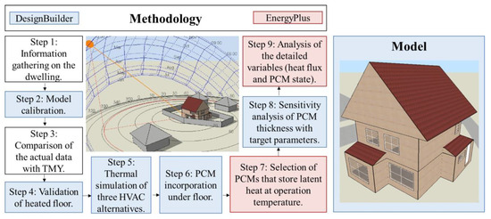
Figure 1.
Workflow steps of the proposed methodology, indicating the simulation software used (DesignBuilder and EnergyPlus), and the 3D model of the case study.
The first step includes collecting the information for the thermal simulation of the existing dwelling (design conditions). When the necessary information was unavailable, we used local standards and norms, as well as international standards [28]. The second step concerns the calibration of the model using the design winter week (critical temperatures). This step allows for the calibration of other design parameters for the simulation, such as set temperatures, air-conditioning, and ventilation schedules. The third step of the proposed workflow is to conduct a comparison of the inner temperatures obtained from the simulation and the actual measured values during a Typical Meteorological Year (TMY). The fourth step is to verify the implementation of the new floor structure and HVAC system “Heated floor v2” using results available in the literature [1,2,3]. The fifth step refers to conducting a thermal simulation of the dwelling with three HVAC alternatives: (i) The actual HVAC system of the existing house (Radiators); (ii) “Heated floor v1” corresponds to incorporating a radiant floor system on the same floor as alternative (i), maintaining the same thermal transmittance (UA); and (iii) “Heated floor v2” corresponds to a radiant floor system with a new structure incorporating a heated floor (wet floor). The sixth step requires incorporating the PCM layer under the radiant floor as a heat source. The analysis involved testing twenty-three PCMs from four manufacturers. These PCMs have melting temperatures between 11 and 44 °C. The seventh step is the selection of PCMs that effectively store latent heat by analyzing whether they undergo phase transitions between the solid and liquid states (PCMs with full operation cycle). The eighth step is the sensitivity analysis of PCM layer thickness, considering three target macroscopic variables: heating gas consumption, carbon emissions, and thermal discomfort hours. Further refinement of the selection of PCM and thickness uses an analysis of detailed variable behavior within the PCM layer. The last step herein is the analysis of the detailed variables. For a representative week of the heating season, detailed variables related to the PCM state were evaluated. Relevant nodes of the PCM layer were analyzed (inner, central, and outer). The analysis of these variables was used to explain the results from the macroscopic variables and propose a selection of PCM and thickness for deployment. Heat flux was analyzed to determine the effect of PCM layer thickness on heat transfer between the PCM layer and the indoors. Also, the evolution of the PCM phase state (solid, liquid, or transition) over time, and the frequency of phase change at representative nodes of the PCM layer, were analyzed.
Description of the Case Study
The case study dwelling is in Chilean Patagonia (Coyhaique), with coordinates 45°35′9.20″ S, 72°2′20.16″ O at 284 m above sea level. Coyhaique has a Cfc climate [29], according to the Koppen classification. This corresponds to a Continental climate, without a dry season and cold summers. Coyhaique has the lowest monthly mean minimum temperature in July (winter) of −3.7 °C and the highest monthly mean maximum temperature in December (summer) of 12.8 °C [30]. The construction information of the two-floor dwelling, with a total built-up area of 102.13 m2, was obtained from the General Ordinance on Urbanism and Construction (OGUC) [28], presented in Table 3.
Table 3.
Construction specifications of the dwelling.
The source of the meteorological data is the SCCY station, classified by the International Civil Aviation Organization and located about 5 km from the house, as presented in Figure 2, from which we obtained the Typical Meteorological Year (TMY) for simulations with DesignBuilder. Additionally, the temperature from the SCCY weather station can be compared with the ReNam information, both in hourly resolution. Indoor housing temperature is available on the National Housing Monitoring Network (ReNaM) [27]. ReNaM is a public database on environmental conditions and energy consumption measurements in housing for research and development. The ReNaM database contains information on 300 dwellings distributed in the Chilean national territory, with 10 located in Coyhaique. The data available from ReNaM includes hourly indoor temperature and relative humidity. This data was measured in hourly resolution (specifically, outdoor temperature) and compared with the same year’s historical data from the SCCY weather station. The cross-checking with both databases revealed 549 missing hourly values, equivalent to 6.27% of the total annual hours. The single house selected from ReNaM corresponded to a detached, wood-based house of 102 [m2] divided into two stories, selected because of the completeness of the measurement dataset, and because its characteristics were deemed as representative of the local building stock.
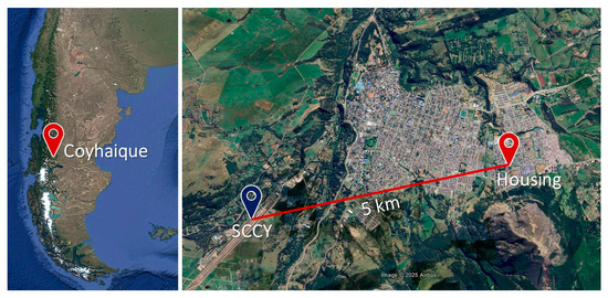
Figure 2.
Location of Coyhaique in Reference to the Southern Tip of South America (left), house location relative to meteorological station SCCY (about 5 km) (right).
The software DesignBuilder v6.1.5.002 and the TMY data from SCCY were used to simulate the dwelling. The national regulations from OGUC provide valuable information about dwelling occupancy and lighting. National and international standards [31,32] provide the required infiltration and ventilation rates. ReNaM contains data about schedules and setpoints for heating. Additionally, these parameters were validated for the critical winter week using data from the dwelling heated by radiators, as in the actual ReNaM house. Based on the temperature data presented in Figure 3, the behavior of the house’s inhabitants was analyzed to adjust the natural ventilation periods, the airflow rate, and the setpoint temperature of the heating system. Two set temperatures were identified for heating, 15 °C (setback) and 25 °C (setpoint), along with their respective operation schedules. In addition, the preferred ventilation schedule and the air change rates resulting from the residents’ daily occupation schedule were also identified. These three ventilation schedules were incorporated as natural ventilation.
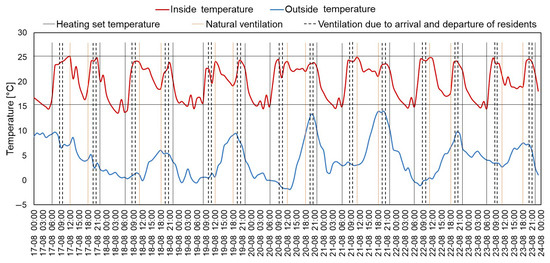
Figure 3.
Calibration of the computational model’s temperature setpoints, ventilation schedule, and air change rates based on the occupants’ behavior during the design winter week.
However, a summary of the daily schedules of occupants, including light, ventilation, infiltration, and heating, is illustrated in Table 4.
Table 4.
Summary of daily schedules of occupants.
The simulations were performed using three different heating systems. The existing dwelling uses radiators for heating, which were modeled using the zone air distribution effectiveness given by ASHRAE Standard 62.1. The second system, “Heated floor v1,” incorporates a heat source (heated floor) under the existing floor to compare both heating systems while maintaining the floor’s constant thermal transmittance (UA). The third, “Heated floor v2,” involves a new floor construction arrangement incorporating the wet heated floor, as illustrated in Figure 4.
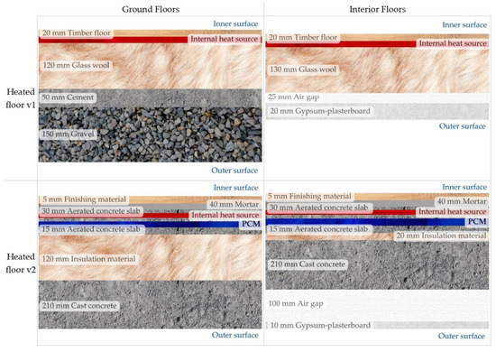
Figure 4.
Soil layering diagram with heat source and PCM. Soil layering of “Radiators” is the same as that of “Heated floor v1”, but without the internal heat source.
Table 5 and Table 6 present the main characteristics of the radiant floor and the floor structure, respectively.
Table 5.
Performances and characteristics of units for hot-water circulation of HVAC heated floor (Made by the authors after [3]).
Table 6.
Construction specifications of the dwelling floor to incorporate a wet heated floor (Heated floor v2).
In all cases, the regularly occupied areas of the dwelling were heated, excluding the unoccupied areas, kitchen, and bathrooms, equivalent to a heated area of 75.52 m2, as presented in Figure 5.
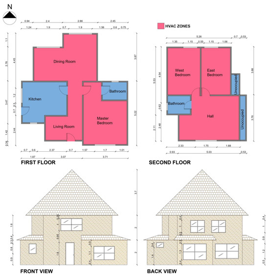
Figure 5.
HVAC zones on the first and second floor (up) and the house’s front and back view (below).
Incorporating the PCM into the floor under the heat source (Heated floor v2) would improve the thermal performance of the heated floor system. The floor structure for this heating system is detailed in Table 7. The effect of PCM incorporation was tested by considering the gas consumption for heating, its associated carbon emissions, and thermal comfort conditions. Twenty-three organic PCMs from four manufacturers with melting temperatures ranging from 11 to 44 °C were considered for analysis. Figure A1, Figure A2 and Figure A3 in Appendix A show the enthalpy–temperature curves for PCMs from the manufacturers RT, BioPCM, and Winco Technologies, while Table A1 in Appendix A describes the thermophysical properties of Infinite R PCM. To the three manufacturers provided in the DesignBuilder database, RT was added [33].
Table 7.
Construction specifications of dwelling floor heating with Heated floor v2 and PCM incorporation.
To incorporate the PCM into the model, an additional layer was included in the floor construction definition in DesignBuilder. The lower images from Figure 4 (Heated floors v2) show the location of the PCM layer (blue section), as seen in the DesignBuilder envelope definition editor. Once incorporated, the material for this layer was selected as one of the PCMs available in the DesignBuilder database. The enthalpy–temperature curves of the different PCMs studied are shown in Appendix A. The simulation updates the specific heat of the PCM layer at each timestep according to its calculated temperature in an iterative process, therefore changing its heat stored or released according to the PCM layer and surrounding surface temperatures. The simulation uses a conduction finite difference model with a space discretization constant of 3, relaxation factor of 1, and inside face surface temperature convergence criteria of 0.002 °C.
The PCMs were analyzed with thicknesses ranging between 5 mm and 60 mm in increments of 5 mm. The phase change behavior of the PCMs was analyzed, and only materials exhibiting phase change during the system’s operation were selected. Finally, for the selected PCMs, the PCM thickness step was reduced between simulation runs, increasing the study’s sensitivity. The temperature–enthalpy charts of the PCMs used are provided in Appendix A.
The analysis of the detailed variables was a computationally intensive process, requiring simulations with minute-by-minute timesteps, to fully capture the changes the material undergoes in front of variable temperatures and operation schedules. Therefore, the detailed analysis was limited to the most promising combinations of PCM and thickness values from the perspective of energy efficiency and thermal comfort. Furthermore, this analysis was limited to representative periods of the heating season, varying between a full week (10 August to 17 August) and two days (10 August to 12 August). The detailed variables were obtained as output variables from the simulation in the EnergyPlus software, enabled with the use of the finite differences algorithm (CondFD) to calculate the heat transfer across the building envelope. These variables were the heat flux and PCM state. The heat flux of relevant nodes within the PCM layer was evaluated between August 10th and August 12th, for different PCM layer-thickness cases. The analysis allowed us to observe the changes in heat flux between the different nodes for two daily working cycles. By comparing different cases, it was possible to understand the effect of PCM and thickness selection on the heat effectively transferred to and from the PCM nodes into the remaining materials of the floor construction. PCM state refers to the phase in which the PCM can be found. This can vary between supercooled solid, solid, transition, liquid, and superheated liquid.
The evolution of this variable between 10 August and 12 August allowed us to determine if a particular PCM was undergoing the full cycle of stages, making use of the heat storage potential, or if it remained in mostly solid or liquid stages. If a PCM remains in a mostly solid condition, it means that its operation temperature tends to remain above the melting temperature, whereas if a PCM remains mostly liquid, it means that the temperatures in the envelope never reach low enough values for the PCM to release the heat stored latently. Both cases signify a misuse of the PCM, which only acts as an additional sensible heat storage medium. A final study based on PCM state analyzed was the phase change frequency. For this variable, the period analyzed comprised a full week between 10 August and 17 August. This analysis measured the number of times in this period when the PCM nodes changed between the 5 stages described earlier. The selected nodes for analysis were the external and internal surfaces of the PCM layer, plus the central node of the layer. This analysis allowed us to determine the adequacy of the PCM operation temperature selection, meaning the onset of temperature swings large enough to generate state changes, and the effect of PCM layer thickness, since by increasing the thickness of the layer its heat transfer resistance also increase, making it more difficult for the nodes further away from the indoors to store or release heat effectively, reducing the number of phase changes.
3. Results and Discussion
3.1. Baseline Validation
To validate the numerical simulation work, the data from the actual house measurements obtained from ReNaM was compared with the simulations in DesignBuilder performed using the Typical Meteorological Year (TMY). To analyze the simulation results, this study began by comparing the representativeness of the temperatures from ReNaM relative to historical data through the cumulative frequency distribution of outdoor temperature and the Earth Mover’s Distance (EMD) metric. The cumulative frequency curves of outdoor temperature (Figure 6, left) showed a strong correlation, reflected in an EMD of 0.014, close to zero, as illustrated in Table 8. The low EMD value indicates that the ReNaM data exhibited typical behavior, validating the comparability of the simulation results using a TMY weather data file with data obtained from the measurements.
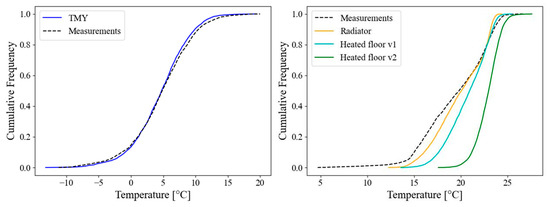
Figure 6.
The cumulative frequency distribution during the heating period for the outdoor temperature (left) and indoor temperature with different HVAC systems (right).
Table 8.
Comparison of cumulative frequency distribution curves using EMD.
Since the actual house is heated with radiators, the “Radiators” simulation was used to compare the indoor temperatures. The simulation resulted in a similar distribution of temperatures (Figure 6, right, yellow vs. black curve) with an EMD of 0.029, as presented in Table 7. The same analysis was conducted for a smaller time window, focusing on eleven representative winter days (July 18–29), as presented in Figure 7 and Figure 8. This analysis was performed to observe divergences that are not appreciable at larger time scales. The EMDs were calculated to be 0.154 for outdoor and 0.049 for indoor temperatures, indicating a more significant divergence in the cumulative frequency curves compared to the annual data, consistent with the reduced time window, although still reasonably low. Figure 8 shows the comparison of the cumulative frequency distributions of outdoor and indoor temperatures for the shorter timeframe, where, despite the differences shown in the time series in Figure 7, the overall range and distribution of temperatures between measurements and simulation are relatable. Therefore, the baseline scenario can be considered as validated with the available measurements.
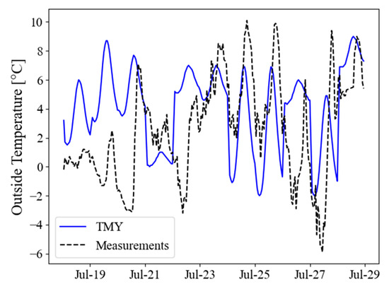
Figure 7.
Hourly outdoor temperature for TMY and year 2018, during a smaller time window (July 18–29).
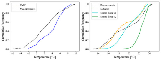
Figure 8.
Cumulative frequency distribution during a smaller time window (July 18–29) for the outdoor temperature (left) and indoor temperature (right).
Verifying the computational implementation of the radiant floor followed the study by Baek and Kim [3] of a house in South Korea. This study obtained a 9.8% difference in the annual energy consumption; however, the thermal transmittance applied in this study was 7.2% higher than that reported by Baek and Kim, as presented in Table 9. This difference was considered acceptable to continue the analysis.
Table 9.
Validation of Heated floor v2.
Replacing radiators with a heated floor enhances comfort conditions inside the house, achieving higher temperatures closer to the target temperature. Including a heat source in the original house floor (“Heated floor v1”) significantly improved indoor temperatures. Subsequently, replacing the house floor with a wet radiant floor (“Heated floor v2”) further enhanced these improvements. The right side of Figure 6 and Figure 8 illustrates the increase in indoor house temperature due to changes of HVAC systems, as shown by a shift in the cumulative frequency curves toward higher temperatures (cyan and green curves). This, in turn, results in an increase in EMD values, as presented in Table 8. The results were analyzed from the perspective of heating gas consumption—and associated carbon emissions—as well as from that of the well-being of the house’s inhabitants, measured as the hours of thermal discomfort for the heated zones. The discomfort hours were calculated directly in DesignBuilder based on ANSI/ASHRAE Standard 55-2017. The results of the heating energy use, emissions, and discomfort hours are presented in Table 10. The baseline case using radiators presents the lowest gas consumption and, consequently, the lowest carbon emissions. However, the heated floor significantly improves the habitability of the dwelling by reducing the hours of thermal discomfort by 94%.
Table 10.
Gas consumption for heating, CO2 equivalent emissions, and discomfort hours for base simulations without PCM inclusion.
3.2. Analysis of Heated Floors with PCM
Next, a grid independence analysis for a PCM-enhanced case is shown. This analysis was performed to determine if the level of discretization used in the baseline case was suitable for the cases enhanced with PCMs, given the higher heat storage capacity of the floor construction. This allows the use of a level of discretization adequate for the task, but no higher, therefore reducing the overall computational cost of the complete study. Zone temperature was selected, since it was the variable used for the calibration with measurements from ReNaM in earlier sections.
The parameter modified in EnergyPlus is the Space Discretization Constant, within the HeatBalanceSettings:ConductionFiniteDifference object, whose values ranged from 3 (baseline case) down to 0.25. The values of the discretization parameter and the associated number of nodes for the complete heated floor construction are shown in Table 11.
Table 11.
Discretization Analysis.
The zone temperature results for the conditioned living area on the first floor of the house are illustrated in Figure 9. The simulation for the three levels of discretization ran between August 10 and August 17.
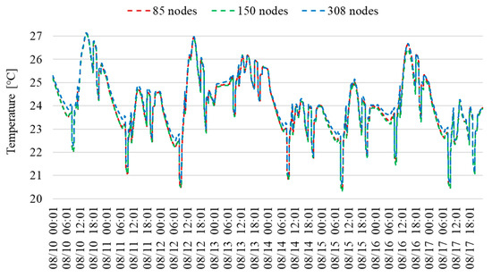
Figure 9.
Indoor temperature with several discretizations.
Figure 9 shows that all cases present a similar behavior, and no significant differences in the maximum and minimum temperature values between different levels of discretization exist; therefore, the use of a Space Discretization Constant value of 3 remains suitable for the cases that include PCM in the floor construction. The maximum absolute differences from the baseline for the cases with 150 and 308 nodes are 0.85% and 0.84%, respectively, while the average absolute differences are 0.18% and 0.21%, respectively.
Considering the melting–solidification cycle analysis, only materials RT38, RT42, and RT44 present full operation cycles for some thicknesses. The main differentiating property of these materials is their nominal phase change temperature corresponding to 38 °C, 42 °C, and 44 °C for RT38, RT42, and RT44, respectively. For the following discussion, the term “full operation cycle” has been defined as a certain PCM undergoing a phase change between solid and liquid phases, not necessarily reaching the superheated or supercooled condition. Therefore, other materials and thickness cases have been excluded from further analysis. The selected cases are shown in Figure 10. It is worth mentioning that none of the PCMs in the DesignBuilder database showed full melting–solidification cycles for heated floor applications, making it necessary to incorporate other PCMs (RT), whose thermophysical properties are presented in Appendix A.
The best-performing material in terms of energy savings is RT42, with a thickness value of 50 mm, reaching up to 2.8% energy savings. However, an inverse relationship between energy savings and reduction in discomfort hours can be observed, with these thicker cases presenting the lowest reduction in thermally comfortable hours for RT42, although still relatively high, between 13.7% and 21%. RT38 shows a behavior less dependent on thickness, with energy savings between 0.5% and 0.7% and a reduction in discomfort between 14.7% and 18.9%. For thickness values below 25 mm, a trend of increasing thermally comfortable hours can be observed as the thickness value increases. RT44 shows the most particular behavior of the selected materials, with drastically different results between 5 mm thickness and values above 10 mm. For a 5 mm thickness, it shows energy savings of around 1.8% and a reduction in discomfort hours close to 27%. However, for 10 mm thickness onwards, RT44 generates increased energy use, ranging between 4.3% and 1.2% above the reference case, with a light trend toward decreasing energy use as thickness increases. Discomfort hours show diminishing improvements over the reference case as the thickness increases over 10 mm, reaching the lowest value of 0.69% reduction for a thickness of 50 mm.

Figure 10.
Absolute values of energy by heating and discomfort hours for selected PCM and thickness values (left) and the variation with respect to the base case, Heated floor v2 (right). A refined parametric analysis was performed for the cases with thickness values below 10 mm, considering thickness increments of 1 mm. The results of this analysis can be seen in Figure 11. RT44 shows a local maximum value of energy savings for the 5 mm thickness, coincident with a local maximum for discomfort hours reduction of 27%. RT38, with a thickness of 1 mm, shows a maximum energy savings of 2% and a discomfort hour reduction of 12.2%. The different tendencies of the energy savings and discomfort hours reduction curves indicate that incorporating PCM into a building envelope is not a simple concern, since it requires careful consideration of the PCM melting and solidification temperatures and the expected operation temperature of the heating system. Additionally, increasing the amount of PCM, aiming to increase the amount of energy that can be stored in it, can reach a situation in which the excess PCM inhibits the fusion and solidification cycles of the material and increases the energy use of the house. The data of Figure 10 and Figure 11 is presented in Table A2 of Appendix A.


Figure 11.
Energy savings and reduction in discomfort hours for thickness values between 1 mm and 10 mm.
Figure 11.
Energy savings and reduction in discomfort hours for thickness values between 1 mm and 10 mm.

To understand the particular behavior of RT44 between the 1 mm and 10 mm thickness values, a deep dive into the heat flux conditions for the PCM layer nodes is required. Figure 12 (left) shows the heat flux values between August 10th and August 12th of node 70 for the cases of 3 mm, 5 mm, and 10 mm thickness. Node 70 represents the center of the PCM layer in all three cases. For the 10 mm case, the values of the heat flux during the heat release periods reach about 50% of the values reached by the 3 mm and 5 mm cases. In these figures, a positive value of heat flux represents heat moving into the node, and negative values represent heat leaving the node. The reduction in heat flux found in the thicker PCM cases can be attributed to the additional thermal resistance of the floor construction, due to the increased thickness of the PCM layer. This reduction in heat transfer to and from the PCM layer limits the amount of heat that actually reaches and is stored in the PCM, thus limiting the heat flux from the PCM nodes during charge and discharge. In contrast, Node 74 in Figure 12 (right) shows a more interior node, further away from the PCM layer. The heat flux values are similar for all cases, which indicates that the effect described can be attributed mostly to the increased thickness of the PCM layer. On the other hand, the differences between the 5 mm case and lower thickness value cases, regarding energy savings, can be attributed to the amount of PCM included. Despite reaching similar values of heat flux, the amount of PCM limits the amount of heat absorbed or released by the PCM layer in the thinner cases. Therefore, the 5 mm case represents a local optimum, given the effects of heat transfer dampening and PCM mass due to the PCM layer thickness described.
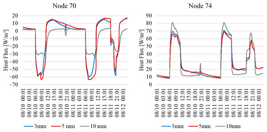
Figure 12.
Heat flux analysis for the central node (node 70, left) and the interior-side node (node 74, right) of the PCM layer.
To analyze the influence of PCM layer thickness on the PCM performance, we obtained minute-by-minute results for the winter week of analysis. Specifically, we focused on two variables, PCM state and heat flux. PCM state indicates the condition of the PCM node at a given instant. As obtained from EnergyPlus v9.5.0, this variable is represented by values that can range between 2 and −2, which represent supercooled solid (solid cooled below the solidification temperature) (2), solid (1), transition (0), liquid (−1), and superheated liquid (liquid heated above the fusion temperature) (−2). This parameter is highly relevant since the ideal operation of a PCM involves undergoing stages of melting, during which the PCM absorbs heat that is released later during the solidification stage. If a PCM does not undergo these cycles, it is not operating as such. This can happen because the PCM may have a melting temperature far from the temperature ranges of the construction elements during the day. This means that the PCM may remain molten or solid throughout the daily temperature cycle of the building. The phase change of the materials cannot be directly observed from the overall energy simulation results of heating energy use and discomfort hours. However, if the amount of heat absorbed or released is not enough to generate a change of state of the PCM at a given temperature condition, only observing the state parameter will reveal no information about the operation of the material. Even considering a partial process not enough to generate a change of state, a PCM can absorb or release a significant amount of heat in the transition between states. Therefore, the complementary variable of heat flux has been considered. This variable represents the amount of heat going through the node, including any internal heat release or absorption.
As an illustration, a comparison of the values of state and heat flux for the PCM layer nodes of the RT 44 case considering PCM layer thickness values of 10 mm and 60 mm is presented. Figure 13 shows the results for the state and heat flux for the external surface node of the PCM layer for both cases over a period between August 10th and August 12th. For example, for the 10 mm thickness case, between 12:01 AM and 06:01 AM on August 12th, the PCM remained in the transition state (0); however, the heat flux indicates active thermal behavior, with oscillations that reveal the material was functioning effectively. The 60 mm case node presents lower absolute values of heat flux and less change in state, remaining between the supercooled solid and solid states. On the other hand, the 10 mm case node shows higher absolute values of heat flux and state cycles ranging between supercooled solid and liquid. The differences in heat flux show that the thicker PCM layer limits the amount of heat that reaches the external node and, therefore, limits heat absorption and release, in comparison to the external node in the 10 mm case, which shows swings of larger magnitude between the charging and discharging stages. This observation coincides with that which can be observed in the state curves, with the additional heat flux that reaches the external node in the 10 mm case leading to more frequent and complete cycles of phase change.
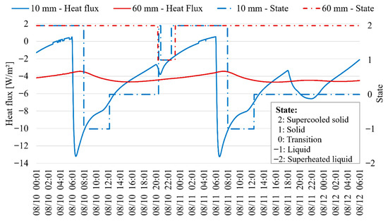
Figure 13.
Comparison of PCM state and heat flux at an external node in the RT 44 case, with layer thicknesses of 10 mm and 60 mm, during the period from 10 August to 12 August.
Considering the analysis period between August 10th and August 17th, Figure 14 shows the frequency of time that each of the nodes remains in each state. The biggest difference can be seen for the external surface node, which, in the case of 10 mm, remains in transition between solid and melted states approximately 60% of the time, whereas in the 60 mm case, it remains in the supercooled liquid state 59% of the time. Also, Table 12 shows the number of state changes over the same period. It can be seen that the 60 mm case presents lower values of state changes than the 10 mm case for all nodes, which indicates that not only does the external node of the 60 mm case spend more time as a supercooled solid, but also that the overall frequency of state change is lower, which negates the benefits of using a PCM. These results indicate that the 60 mm case presents underutilized PCM mass, which, considering its costs, may lead to the existence of a point of diminishing returns regarding the amount of PCM included, and the amount of heat stored and released during the fusion–solidification cycles of the material.
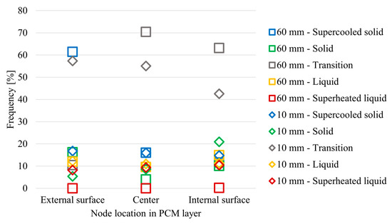
Figure 14.
Frequency of time that each node (external, central, and internal) remains in each state for PCM layer thicknesses of 10 mm and 60 mm during the period from 10 August to 17 August.
Table 12.
Comparison of the number of state changes of PCM RT44 for layer thicknesses of 10 mm and 60 mm during the period from 10 August to 17 August.
The inverse relationship between energy savings and reduction in discomfort hours can be seen in Figure 10 for RT 42 and RT 44, although in the case of RT 44, cases between 10 mm and 50 mm thickness do not reach positive energy savings. As discussed in the analysis of RT 44 with thickness values between 1 mm and 10 mm, the thickness of the PCM layer appears to impact the heat transfer conditions in the material. Specifically, at higher thickness values, the heat released by the PCM decreases. This reduction is not seen in nodes of layers closer to the indoors. This indicates that the thickness of the PCM layer thermally insulates the PCM from the indoors.
Figure 13 and Figure 14 reinforce this takeaway, showing that for higher PCM thickness, the PCM shows lower values of heat flux, dampened by the relatively low thermal conductivity of the thicker PCM layer, and thus experiences fewer, if any, cycles of melting and solidification. However, despite not operating as intended, the thicker PCM layer increases the overall thermal inertia of the construction, effectively increasing the amount of energy it can store. Therefore, the thinner cases can present the opportunity for the stabilization of temperatures during the more frequent phase change stages, at the cost of lower total energy stored. This explains the divergence in behavior between the curves of energy savings and reduction in discomfort hours as functions of PCM thickness. Given the relatively high level of thermal insulation and the location of the PCM closer to the indoors, the effects of outdoor temperatures can be considered unlikely to be the drivers of this behavior, along with the operation conditions of the HVAC system, this being the same for all cases.
4. Conclusions
This study evaluated the feasibility of using a radiant floor heating system enhanced by a PCM integrated in the floor structure, studying detailed variables related to PCM state to provide additional information beyond that of commonly used macroscopic variables. This methodology allowed the identification of combinations of PCM selection and thickness that maximize the use of PCM heat storage potential, and also the identification of cases where the macroscopic variables showed desirable results, but the PCM heat storage capabilities were not being fully utilized, therefore leading to a misuse of expensive PCM. The three final PCMs selected achieved comparable maximum energy saving values, though at different thicknesses. The most significant heating reduction (and, consequently, carbon emission reduction) was achieved for melting temperatures of 42 °C (RT42). Among the scenarios simulated, a 50 mm layer of RT42 reached the highest energy savings (2.8%) and highest carbon emission reduction (2.4%) with a reduction in discomfort hours of 19%. In comparison, the highest discomfort hours reduction (27%) was reached with a layer of 4 mm of RT44, with energy saving and carbon emission reduction of 1.3% and 1.1%, respectively. Considering simultaneously the amount of PCM, heating energy savings, and reduction in thermal discomfort, the use of a layer of 5 mm of RT44 emerges as a particularly effective alternative. It achieves energy savings, carbon emission reductions, and discomfort hours reductions of 1.8%, 1.5%, and 27%, respectively—matching the greatest reduction in discomfort hours among all the cases studied.
The study demonstrated that the proposed methodology, combining detailed variables such as PCM state, heat flux, and temperature with macroscopic indicators like heating energy use and indoor comfort, effectively explains the behavior of PCM-enhanced heated floors. Validation of the baseline house model against on-site ReNaM measurements yielded an EMD as low as 0.048 for the full heating season, confirming the reliability of subsequent simulations. Results showed that while PCMs can reduce thermal discomfort hours by up to 27% and achieve notable energy savings and carbon-emission reductions, their performance depends strongly on melting temperature and layer thickness. Some PCM–thickness combinations failed to complete melting–solidification cycles, underscoring the need for detailed state analysis to reveal latent heat storage limitations that macroscopic variables alone cannot detect.
Among the materials studied, RT42 achieved the greatest energy savings (2.8%) at 50 mm, whereas RT44 provided the largest comfort improvement, reducing discomfort hours most effectively at 4–5 mm. RT38 reached a 2% energy saving peak at only 1 mm. Overall, thinner PCM layers tended to produce higher comfort gains, but no single material or thickness simultaneously maximized both comfort and efficiency, revealing an inverse relationship between these outcomes. Consequently, the optimal selection of PCM type and thickness requires a case-specific trade-off analysis that balances energy efficiency, thermal comfort, and material cost.
Despite the favorable results from the validation of the baseline scenario with the measured data from ReNaM, and the comparison of the heated floor with data from the literature, the results of the PCM cases shown herein remain to be validated with experimental data. Such work would require generating a laboratory setup containing the heated floor enhanced with PCMs, and replicating the operation of the actual house. This validation could be used to calibrate the models and strengthen the takeaways from the study.
The success of the energy efficiency and thermal comfort measures described herein may enable further improvements at the energy community level. For example, a residential community using heated floors enhanced with PCMs could satisfy its heating needs using hot water provided by a heat pump-based thermal plant. Heat pumps can operate at higher energy efficiency than fuel-based boilers. In addition, they do not generate local particulate matter emissions, which addresses the environmental needs of Coyhaique. Therefore, the energy savings from individual homes can amount to significant values of heating power when considering a complete district heating system, making the interventions economically feasible. Furthermore, the relatively small thermal comfort improvement due to the PCM enhancement can act as a side benefit to the energy savings at the system level, to facilitate the final user acceptance of the retrofit and district heating plans.
Author Contributions
Conceptualization, N.O., T.V. and D.A.V.; methodology, N.O., A.C.-B., T.V. and D.A.V.; software, N.O., A.C.-B. and T.V.; validation, N.O. and T.V.; formal analysis, N.O., A.C.-B., T.V., B.B.F.d.C., M.K.N., A.N.H. and D.A.V.; investigation, N.O., T.V. and D.A.V.; resources, B.B.F.d.C., M.K.N., A.N.H. and D.A.V.; data curation, N.O. and T.V.; writing—original draft preparation, N.O., T.V. and D.A.V.; writing—review and editing, N.O., A.C.-B., T.V., B.B.F.d.C., M.K.N., A.N.H. and D.A.V.; visualization, N.O., A.C.-B. and T.V.; supervision, A.N.H. and D.A.V.; project administration, D.A.V.; funding acquisition, D.A.V. All authors have read and agreed to the published version of the manuscript.
Funding
This research was funded by Agencia Nacional de Investigación y Desarrollo, ANID Chile, Proyecto FONDECYT N° 1201520, Proyecto FONDECYT N° 1251661, and Proyecto ANILLO N° ACT240015. Tomás Venegas received funding from Vicerrectoría de Investigación, Innovación y Creación, Universidad de Santiago de Chile, Postdoctoral Research Project POSTDOC_DICYT, Código 092416VC_Postdoc.
Data Availability Statement
The original contributions presented in this study are included in the article. Further inquiries can be directed to the corresponding author.
Acknowledgments
Natalia Osorio extends her gratitude to Johanna Ulloa for her guidance on construction-related matters and her assistance with the architectural plans. Mohammad Najjar and Assed Haddad would like to acknowledge the support of Conselho Nacional de Desenvolvimento Científico e Tecnológico (CNPq 304726/2021-4), and Fundação Carlos Chagas Filho de Amparo à Pesquisa do Estado do Rio de Janeiro (FAPERJ E-26400.205.206/2022 (284891)) and (FAPERJ E-26/210.569/2025 (305234)), which helped in the development of this research.
Conflicts of Interest
The authors declare no conflict of interest.
Appendix A

Figure A1.
Partial enthalpy–Temperature of RT-PCMs. Thermal conductivity = 0.2 W/m K, specific heat = 2000 J/kg K, density = [750–825] kg/m3.
Figure A1.
Partial enthalpy–Temperature of RT-PCMs. Thermal conductivity = 0.2 W/m K, specific heat = 2000 J/kg K, density = [750–825] kg/m3.

Table A1.
Phase Change Properties of Infinite R PCM.
Table A1.
Phase Change Properties of Infinite R PCM.
| Latent heat during the entire phase change [kJ/kg] | 200 | |||||
| Density [kg/m3] | 1540 | |||||
| Specific heat [J/kg K] | 3140 | |||||
| Thermal conductivity [W/m K] | Liquid state | Solid state | ||||
| 0.54 | 1.09 | |||||
| Melting and freezing curve | I18 | I21 | I23 | |||
| Melting | Freezing | Melting | Freezing | Melting | Freezing | |
| Peak temperature [°C] | 19 | 17 | 22 | 20 | 24 | 22 |
| High temperature difference [°C] | 1 | 1 | 1 | |||
| Low temperature difference [°C] | 1 | 1 | 1 | |||

Figure A2.
Enthalpy–Temperature of BioPCMs. Thermal conductivity = 0.2 W/m K, specific heat = 1970 J/kg K, density = 235 kg/m3.
Figure A2.
Enthalpy–Temperature of BioPCMs. Thermal conductivity = 0.2 W/m K, specific heat = 1970 J/kg K, density = 235 kg/m3.


Figure A3.
Enthalpy–temperature of Winco Technologies Enerciel-PCMs. Thermal conductivity = 0.148 W/m K, specific heat = 2500 J/kg K, density = 832 kg/m3.
Figure A3.
Enthalpy–temperature of Winco Technologies Enerciel-PCMs. Thermal conductivity = 0.148 W/m K, specific heat = 2500 J/kg K, density = 832 kg/m3.

Table A2.
Gas consumption for heating, CO2 equivalent emissions, and discomfort hours for base simulations with PCMs inclusion. Case base without PCM corresponds to PCM thickness = 0.
Table A2.
Gas consumption for heating, CO2 equivalent emissions, and discomfort hours for base simulations with PCMs inclusion. Case base without PCM corresponds to PCM thickness = 0.
| RT 38 | RT 42 | RT 44 | |||||||
|---|---|---|---|---|---|---|---|---|---|
| Gas for Heating | CO2 Emissions | Discomfort | Gas for Heating | CO2 Emissions | Discomfort | Gas for Heating | CO2 Emissions | Discomfort | |
| PCM Thickness | kWh | kg | Hours | kWh | kg | Hours | kWh | kg | Hours |
| 0 | 12,961 | 2913 | 117 | 12,961 | 2913 | 117 | 12,961 | 2913 | 117 |
| 1 | 12,704 | 2864 | 108 | 12,741 | 2871 | 103 | 12,838 | 2890 | 101 |
| 2 | 12,780 | 2879 | 105 | 12,825 | 2887 | 100 | 12,966 | 2914 | 95 |
| 3 | 12,823 | 2887 | 103 | 12,862 | 2894 | 96 | 12,931 | 2907 | 90 |
| 4 | 12,849 | 2892 | 101 | 12,869 | 2895 | 93 | 12,794 | 2881 | 85 |
| 5 | 12,866 | 2895 | 100 | 12,862 | 2894 | 92 | 12,730 | 2869 | 85 |
| 6 | 12,879 | 2897 | 99 | 12,848 | 2891 | 91 | 12,796 | 2882 | 90 |
| 7 | 12,887 | 2899 | 98 | 12,835 | 2889 | 91 | 12,958 | 2912 | 98 |
| 8 | 12,893 | 2900 | 98 | 12,824 | 2887 | 92 | 13,267 | 2971 | 102 |
| 9 | 12,897 | 2901 | 97 | 12,813 | 2885 | 93 | 13,568 | 3028 | 112 |
| 10 | 12,893 | 2900 | 97 | 12,797 | 2882 | 93 | 13,514 | 3017 | 112 |
| 12 | 12,892 | 2900 | 97 | 12,777 | 2878 | 94 | 13,471 | 3009 | 113 |
| 14 | 12,888 | 2899 | 97 | 12,757 | 2874 | 95 | 13,436 | 3002 | 113 |
| 15 | 12,883 | 2898 | 96 | 12,746 | 2872 | 95 | 13,400 | 2996 | 113 |
| 16 | 12,882 | 2898 | 96 | 12,737 | 2870 | 96 | 13,384 | 2993 | 113 |
| 18 | 12,879 | 2897 | 96 | 12,721 | 2867 | 96 | 13,355 | 2987 | 113 |
| 20 | 12,876 | 2897 | 95 | 12,705 | 2864 | 97 | 13,319 | 2980 | 114 |
| 25 | 12,871 | 2896 | 95 | 12,673 | 2858 | 98 | 13,262 | 2969 | 114 |
| 30 | 12,868 | 2895 | 95 | 12,647 | 2853 | 99 | 13,220 | 2962 | 114 |
| 35 | 12,866 | 2895 | 95 | 12,626 | 2849 | 100 | 13,187 | 2955 | 115 |
| 40 | 12,863 | 2894 | 95 | 12,613 | 2847 | 101 | 13,160 | 2950 | 115 |
| 45 | 12,861 | 2894 | 95 | 12,602 | 2845 | 101 | 13,137 | 2946 | 116 |
| 50 | 12,859 | 2893 | 95 | 12,594 | 2843 | 101 | 13,117 | 2942 | 116 |
References
- Baek, S.; Park, J.C. Proposal of a PCM Underfloor Heating System Using a Web Construction Method. Int. J. Polym. Sci. 2017, 2017, 2693526. [Google Scholar] [CrossRef]
- Baek, S.; Kim, S. Determination of optimum hot-water temperatures for PCM radiant floor-heating systems based on thewet construction method. Sustainability 2018, 10, 4004. [Google Scholar] [CrossRef]
- Baek, S.; Kim, S. Analysis of thermal performance and energy saving potential by PCM radiant floor heating system based on wet construction method and hot water. Energies 2019, 12, 828. [Google Scholar] [CrossRef]
- Sun, W.; Zhang, Y.; Ling, Z.; Fang, X.; Zhang, Z. Experimental investigation on the thermal performance of double-layer PCM radiant floor system containing two types of inorganic composite PCMs. Energy Build. 2020, 211, 109806. [Google Scholar] [CrossRef]
- Rebelo, F.; Figueiredo, A.; Vicente, R.; Almeida, R.; Paiva, H.; Ferreira, V. Development of innovative mortars incorporating phase change materials and by-products for high performance radiant floor systems. Constr. Build. Mater. 2024, 420, 135488. [Google Scholar] [CrossRef]
- Liu, Z.; Wei, Z.; Teng, R.; Sun, H.; Qie, Z. Research on performance of radiant floor heating system based on heat storage. Appl. Therm. Eng. 2023, 231, 120812. [Google Scholar] [CrossRef]
- Larwa, B.; Cesari, S.; Bottarelli, M. Study on thermal performance of a PCM enhanced hydronic radiant floor heating system. Energy 2021, 225, 120245. [Google Scholar] [CrossRef]
- Plytaria, M.T.; Tzivanidis, C.; Bellos, E.; Antonopoulos, K.A. Antonopoulos, Energetic investigation of solar assisted heat pump underfloor heating systems with and without phase change materials. Energy Convers. Manag. 2018, 173, 626–639. [Google Scholar] [CrossRef]
- Babaharra, O.; Choukairy, K.; Hamdaoui, S.; Khallaki, K.; Mounir, S.H. Thermal behavior evaluation of a radiant floor heating system incorporates a microencapsulated phase change material. Constr. Build. Mater. 2022, 330, 127293. [Google Scholar] [CrossRef]
- Belete, M.B.; Murimi, E.; Muiruri, P.I.; Munyalo, J. A comprehensive experimental characterization of cement mortar containing sodium sulfate dehydrate/calcium chloride hexahydrate/graphite shape-stable PCM for enhanced thermal regulation in buildings. Results Eng. 2024, 22, 102028. [Google Scholar] [CrossRef]
- Bohórquez-Órdenes, J.; Tapia-Calderón, A.; Vasco, D.A.; Estuardo-Flores, O.; Haddad, A.N. Methodology to reduce cooling energy consumption by incorporating PCM envelopes: A case study of a dwelling in Chile. Build. Environ. 2021, 206, 108373. [Google Scholar] [CrossRef]
- Comisión Nacional de Energía de Chile. Balance Energético 2022. 2022. Available online: http://energiaabierta.cl/categorias-estadistica/balance-energetico/ (accessed on 16 July 2024).
- Porras-Salazar, J.; Contreras-Espinoza, S.; Cartes, I.; Piggot-Navarrete, J.; Pérez-Fargallo, A. Energy poverty analyzed considering the adaptive comfort of people living in social housing in the central-south of Chile. Energy Build. 2020, 223, 110081. [Google Scholar] [CrossRef]
- Cortés, A.; Amigo, C. Energy culture and the dynamics of energy poverty in south Chile: A blind spot for decontamination energy efficiency policies. People Place Policy Online 2022, 16, 73–97. [Google Scholar] [CrossRef]
- Pérez-Fargallo, A.; Bienvenido-Huertas, D.; Rubio-Bellido, C.; Trebilcock, M. Energy poverty risk mapping methodology considering the user’s thermal adaptability: The case of Chile. Energy Sustain. Dev. 2020, 58, 63–77. [Google Scholar] [CrossRef]
- Pérez-Fargallo, A.; Marín-Restrepo, L.; Contreras-Espinoza, S.; Bienvenido-Huertas, D. Do we need complex and multidimensional indicators to assess energy poverty? The case of the Chilean indicator. Energy Build. 2023, 295, 113314. [Google Scholar] [CrossRef]
- Urquiza, A.; Amigo, C.; Billi, M.; Calvo, R.; Labraña, J.; Oyarzún, T.; Valencia, F. Quality as a hidden dimension of energy poverty in middle-development countries. Literature review and case study from Chile. Energy Build. 2019, 204, 109463. [Google Scholar] [CrossRef]
- Ministerio del Medio Ambiente. Plan de Descontaminación Atmosférica para la Ciudad de Coyhaique y su Zona Circundante; Ministerio del Medio Ambiente: Santiago, Chile, 2019; pp. 1–27. Available online: https://www.diarioficial.cl (accessed on 1 November 2025).
- Tian, C.; Ahmad, N.A.; Rased, A.N.N.W.A.; Wang, S.; Tian, H. Establishing energy-efficient retrofitting strategies in rural housing in China: A systematic review. Results Eng. 2024, 24, 103653. [Google Scholar] [CrossRef]
- ANSI/ASHRAE Standard 55-2017; American Society of Heating, Refrigerating, and Air Conditioning Engineers: Peachtree Corners, GA, USA, 2017. Available online: https://www.ashrae.org/technology (accessed on 1 November 2025).
- Oravec, J.; Šikula, O.; Krajčík, M.; Arıcı, M.; Mohapl, M. A comparative study on the applicability of six radiant floor, wall, and ceiling heating systems based on thermal performance analysis. J. Build. Eng. 2021, 36, 102133. [Google Scholar] [CrossRef]
- Zhang, D.; Cai, N.; Wang, Z. Experimental and numerical analysis of lightweight radiant floor heating system. Energy Build. 2013, 61, 260–266. [Google Scholar] [CrossRef]
- Werner-Juszczuk, A.J.; Siuta-Olcha, A. Assessment of the impact of setting the heating curve on reducing gas consumption in a residential building while ensuring thermal comfort. J. Build. Eng. 2024, 94, 110032. [Google Scholar] [CrossRef]
- Wang, Q.; Ploskić, A.; Holmberg, S. Retrofitting with low-temperature heating to achieve energy-demand savings and thermal comfort. Energy Build. 2015, 109, 217–229. [Google Scholar] [CrossRef]
- Yang, X.; Pan, L.; Guan, W.; Tian, Z.; Wang, J.; Zhang, C. Optimization of the configuration and flexible operation of the pipe-embedded floor heating with low-temperature district heating. Energy Build. 2022, 269, 112245. [Google Scholar] [CrossRef]
- Karakoyun, Y.; Acikgoz, O.; Kucukyildirim, B.O.; Yumurtaci, Z.; Dalkilic, A.S. An experimental investigation on the effect of use of nanofluids in radiant floor heating systems. Energy Build. 2021, 252, 111406. [Google Scholar] [CrossRef]
- Fundación Chile-Minvu. Red Nacional de Monitoreo de Viviendas–ReNaM. 2018. Available online: https://csustentable.minvu.gob.cl/item/red-de-monitoreo/ (accessed on 21 August 2021).
- Ministerio de Vivienda y Urbanismo. Ordenanza General de Urbanismo y Construcciones (OGUC). 2006. Available online: https://www.minvu.cl/elementos-tecnicos/decretos/d-s-n47-1992-ordenanza-general-de-urbanismo-y-construcciones-actualizada-a-22-febrero-2018/ (accessed on 16 August 2021).
- Beck, H.E.; Zimmermann, N.E.; McVicar, T.R.; Vergopolan, N.; Berg, A.; Wood, E.F. Present and future köppen-geiger climate classification maps at 1-km resolution. Sci. Data 2018, 5, 180214. [Google Scholar] [CrossRef]
- Castillo Fontannaz, C. Estadística Climatología. Tomo III; Dirección Meteorológica de Chile: Santiago, Chile, 2001. [Google Scholar]
- ANSI/ASHRAE 62.1; Ventilation for Acceptable Indoor Air Quality. American Society of Heating, Refrigerating and Air-Conditioning Engineers, Inc.: Peachtree Corners, GA, USA, 2007. Available online: https://www.ashrae.org (accessed on 16 August 2021).
- NCh 3309; Ventilacion—Calidad de aire interior aceptable en edificios residenciales de baja altura. Instituto Chileno de Normalizacion: Santiago, Chile, 2014. Available online: https://www.inn.cl (accessed on 29 June 2024).
- Rubitherm Technologies GmbH, PCM RT-Line, Product Table. 2025. Available online: https://www.rubitherm.eu/en/productcategory/organische-pcm-rt (accessed on 21 January 2025).


Disclaimer/Publisher’s Note: The statements, opinions and data contained in all publications are solely those of the individual author(s) and contributor(s) and not of MDPI and/or the editor(s). MDPI and/or the editor(s) disclaim responsibility for any injury to people or property resulting from any ideas, methods, instructions or products referred to in the content. |
© 2025 by the authors. Licensee MDPI, Basel, Switzerland. This article is an open access article distributed under the terms and conditions of the Creative Commons Attribution (CC BY) license (https://creativecommons.org/licenses/by/4.0/).