Predicting the Strength of Heavy Concrete Exposed to Aggressive Environmental Influences by Machine Learning Methods

Abstract

Currently, intelligent algorithms are becoming a reliable alternative source of data analysis in many areas of human activity. In materials science, the integration of machine learning methods is effectively applied to predictive modeling of building materials properties. This is particularly interesting and relevant for predicting the strength properties of building materials under aggressive environmental conditions. In this study, machine learning methods (Linear Regression, K-Neighbors, Decision Tree, Random Forest, CatBoost, Support Vector Regression, and Multilayer Perceptron) were used to analyze the relationship between the strength properties of heavy concrete depending on the freeze–thaw cycle, the average area of damaged areas during this cycle, and the number of damaged areas. The Random Forest and CatBoost methods demonstrate the smallest errors: deviations from actual values are 0.27 MPa and 0.25 MPa, respectively, with an average absolute percentage error of less than 1%. The determination coefficient R² for both models is greater than 0.99. High values of this statistical measure indicate that the implemented models adequately describe changes in the observed data. The theoretical and practical development of intelligent algorithms in materials science opens up vast opportunities for the development and production of materials that are more resistant to aggressive influences.

1. Introduction

Artificial intelligence (AI) is currently a vital tool for automating processes in various areas of human activity [1,2,3,4]. The construction industry, which is characterized by the predominant use of traditional methods, is also gradually seeing an increase in intelligent solutions [5,6,7]. Acting as complementary tools, new smart solutions are often equal in quality and accuracy and significantly outperform existing classical algorithms in speed [8,9].

AI methods, particularly machine learning, have found application in ensuring safety during construction work [10]. The implementation of novel technologies to improve construction safety and promote health has been particularly accelerated during the pandemic [11,12]. However, even after the end of the pandemic and the return of construction regulations to previous standards, intelligent technologies have firmly established themselves in the construction industry as a means of control [13,14,15,16]. A multi-tasking approach based on computer vision technologies for improved construction safety monitoring was considered. Systems were developed to identify unsafe work practices on construction sites proactively [17,18,19]. Risks arise at various stages of the construction process, the analysis of which is now often entrusted to intelligent systems [20,21]. Timely analysis helps minimize losses and improve the quality of construction processes. AI methods offer promising solutions for improving risk management by identifying their frequency and consequences and comparing them with different risk categories in previous projects [22,23].

Computer vision systems have become widespread in the construction industry [24,25,26,27,28]. Binary crack detection in concrete infrastructure was the subject of a comparative analysis of three deep learning architectures. Carefully selected lightweight convolutional neural network architectures demonstrated 95% accuracy, providing reliable crack detection in real time [29]. Deep neural network architectures are used to analyze 3D data, improving a variety of construction processes, from determining the flakiness of crushed stone to the restoration and reconstruction of buildings [30,31]. Structural health monitoring (SHM), which allows for the recording of damage to buildings and structures and the identification of negative factors that can lead to destruction, is currently being implemented, among other things, using AI methods. Machine learning (ML) and deep learning (DL) can be used to detect anomalies and identify damage, optimize maintenance schedules, and prevent failures [32,33,34,35].

In the field of predicting physical and mechanical properties, AI methods can reveal hidden patterns in data sets, providing a high-quality basis for further decision-making [36,37,38,39,40,41]. High efficiency (coefficient of determination (R²) was equal 0.99 for predicted and actual values) has been achieved in predicting the self-compacting concrete compressive strength using artificial neural networks [42]. The compressive strength of concrete was predicted using machine learning algorithms based on CatBoost gradient boosting, k-nearest neighbors, and support vector regression. The best model demonstrated the following values of quality metrics: MAE = 1.97, MSE = 6.85, RMSE = 2.62, MAPE = 6.15, determination coefficient R² = 0.99 [43]. Prediction of the strength properties of concrete with different additives is also possible using AI [44,45,46]. For example, the strength of fly ash-based concrete was determined using a fully connected ANN, a convolutional neural network and a hybrid model, as well as several transform models. The determination coefficient for the best models ranged from 0.95 to 0.97 [47]. Several machine learning algorithms were used to ascertain the strength of concrete with waste glass powder: linear regression (LR), K-nearest neighbors regressor (KNN), ElasticNet regression (ENR), decision tree regressor (DT), random forest regressor (RF) and support vector regressor (SVR). With an R² of 0.95 and an RMSE of 3.40 MPa [48], SVR displayed superior accuracy and predictive performance compared to the other algorithms examined.

Solving regression problems in the field of predictive modeling of the properties of building materials is also possible taking into account the aggressive impact of the environment. The compressive strength prediction in concrete facilities with powdered waste exposed to high temperatures using machine learning has already been studied [49]. The XGB model achieved the highest R² value of 0.9989, in addition to the lowest prediction errors: MAE = 0.1351 MPa, RMSE = 0.1842 MPa, and MAPE = 0.48%.

Predicting the strength of concrete exposed to various types of aggressive impacts is essential for understanding the application, potential service life of the material, and the dynamics of deterioration of its mechanical properties. This requires investigating the behavior of concrete not only at high temperatures but also under freeze–thaw cycles [50,51] and other impacts [52]. Previous studies have addressed the prediction of concrete strength under freeze–thaw cycles, the comparison of several machine learning methods, and the identification of the most effective ones rather succinctly. Such studies are few and far between, which is undoubtedly a gap that is addressed in this study and represents its novelty. This study fills the gap in the research on methods for predicting the strength of heavy concrete under aggressive environments using intelligent methods (predictive models and computer vision).

The objective of the study is to develop machine learning models for predicting the strength of heavy concrete under aggressive environmental conditions. Freeze–thaw cycles are considered as an aggressive impact. The average area of damaged areas and their number, determined using computer vision, are considered as factors influencing strength.

Research objectives:

-

Conduct laboratory studies and tests;

-

Generate a dataset based on test results;

-

Select, implement, and train machine learning models;

-

Evaluate quality metrics;

-

Develop practical recommendations for using the developed models.

The study includes the following sections:

• Introduction, which provides an overview of the subject area, intelligent solutions in the construction industry, and existing gaps.
• The Materials and Methods (Section 2) describes the study process (described by the pipeline), the data used, and the intelligent algorithms.
• The “Results and discussion” (Section 3) details the implementation of machine learning algorithms, analyzes the resulting quality metrics, and compares them with existing work by other researchers in this field.
• Conclusions contains the main findings of the study and outlines plans for further development of this research.

2. Materials and Methods

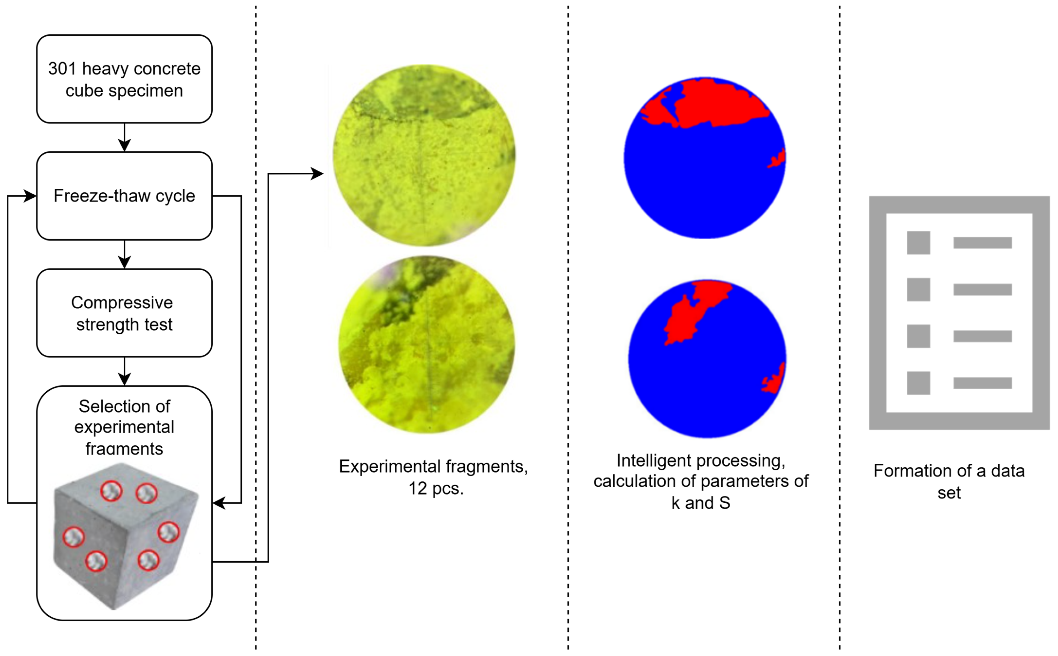
Figure 1 shows the research pipeline, which includes six steps:

• Conducting laboratory tests.
• Dataset formation.
• Exploratory data analysis (EDA).
• Selection and creation of AI models.
• Evaluation of quality metrics.
• Practical recommendations.

Figure 1. Research Pipeline.

2.1. Conducting Laboratory Tests

For the study, 301 cube specimens were manufactured from heavy-weight concrete.

The concrete mix proportions for 1 m³ are as follows: PC—340 kg/m³; water—190 L/m³; KS—690 kg/m³; CrS—1090 kg/m³; PA—3.5 kg/m³, water–cement ratio—0.56, curing conditions: air temperature 20 ± 2 °C, relative air humidity—95 ± 5 °C.

The preparation of laboratory samples was conducted in compliance with current regulatory and technical documentation. Following a 28-day curing period under typical conditions, the specimens underwent freeze–thaw cycles in compliance with GOST 10060 [53]. A special feature of the research methodology was the compressive strength test of one cube daily, with the exception of the control specimen, which was subjected to the strength test immediately, without freeze–thaw cycles.

After each freeze–thaw cycle, 12 test concrete fragments were collected from the broken cube. A photographic record of the specimens was made using an MBS-10 microscope (Izmeritelnaya Tekhnika, St. Petersburg, Russia). In a number of samples, structural damage was observed due to the expansion of freezing water within the pores and cracks of the material, leading to internal stresses in the concrete. This damage was observed as microcracks, material delamination, or structural rupture (fracture). At magnification up to 100×, microcracks and material delamination were visible, as well as the first signs of future structural failure of the concrete.

2.2. Formation of Dataset

Each test fragment was run through a computer vision-based algorithm to determine the number of damaged areas and their average area. The computer vision algorithm runs the image through a U-Net convolutional neural network, accompanied by a “cellular automaton algorithm” (Precision = 0.910, Recall = 0.91, F1 = 0.915, IoU = 0.85, and Accuracy = 0.906).

The detected number is recorded in the values of the k parameter in the resulting dataset, and $S_{Ci}$—the average damage area in the i-th cycle—is calculated using the formula:

$$S_{Ci}={\displaystyle \sum _{j=1}^{12}\frac{S_j}{12}}$$

(1)

where i = 0, …, 300; and Sj is the damage area in fragment j.

Figure 2 shows a visualization of the calculation process for parameters S and k.

Figure 2. Steps for obtaining a dataset.

It is worth noting that the U-Net convolutional neural network was trained, validated, and tested using 500 images. The images fully correspond to the results obtained in laboratory tests. The images reflect disruptions in the integrity and compactness of the particle packing filling the cement matrix of heavy-duty concrete exposed to aggressive environmental conditions.

Before feeding the data into the computer vision models, an experienced technologist annotated the images. These factors indicate a high degree of confidence in the results obtained from data processing using the proposed approach.

Particular attention should be paid to the methodological approach to conducting the experiment and collecting data for use in intelligent algorithms. To this end, the laboratory experiment was methodologically broken down into finite elements, each comprising a single cycle. Each cycle was assessed as a factor influencing the final characteristics of the material.

After conducting physical experiments on 301 cube specimens, we obtained a relationship between the number of freeze–thaw cycles and concrete parameters.

The resulting relationships are sufficient and detailed, allowing us to extrapolate and use literature data to determine parameter values for 300–600 cycles.

This ensured the highest possible accuracy of the experiment and the experimental data for constructing algorithms. The resulting dataset is the first iteration in a series of studies devoted to the influence of aggressive environments on strength characteristics. Subsequent addition of new properties and refinement of existing dependencies will allow for the best possible approximation of real-world conditions.

The resulting dataset of 600 specimens served as a database for further intelligent analysis. The resulting dataset is a table consisting of the following columns:

-

F, freeze–thaw cycle;

-

S, average area of damaged areas;

-

k, number of damaged areas;

-

R_b, specimen strength.

Thus, this study analyzed the dependances between the strength properties of heavy-weight concrete and the freeze–thaw cycle, the average of damaged areas during this cycle, and the number of damaged areas.

2.3. Exploratory Data Analysis (EDA)

After collecting the dataset, it must be thoroughly analyzed (Exploratory Data Analysis) to check for missing, invalid, and null values, as well as for noise and outliers. Table 1 presents a statistical summary for each column of the analyzed dataset.

Table 1. Descriptive Statistics of the Data.

Statistical Parameter	Rb, МПа	F, Cycle	Average Damage Area (S), mm2	Number of Areas (k)
count	351	351	351	351
mean	37.52	193.16	6.26	7.39
std	7.45	137.15	4.23	6.41
min	13.1	0	2	2
25%	36.95	87.5	4	3
50%	39.9	175	5	5
75%	42.2	262.5	7	8
max	43.5	600	25	34

The number of samples in each column is the same—351. The “mean” row shows the mean values: the average strength of the building material samples under consideration was 37.52 MPa, the average strength of the detected damage was 6.26 mm², and the average number of areas was 7.39. The table also shows that the minimum strength was 13.1 MPa, the maximum 43.5 MPa, and the area ranged from 2 to 25 mm². Under aggressive conditions, the number of damaged areas ranged from 2 to 34.

The data presented in Table 1 are consistent with the actual behavior of concrete in aggressive environments. Increasing the number of freeze–thaw cycles leads to an increase in the damaged area and the number of damaged areas, necessitating the creation of heavy-duty concrete with increased strength properties and reserve porosity [54].

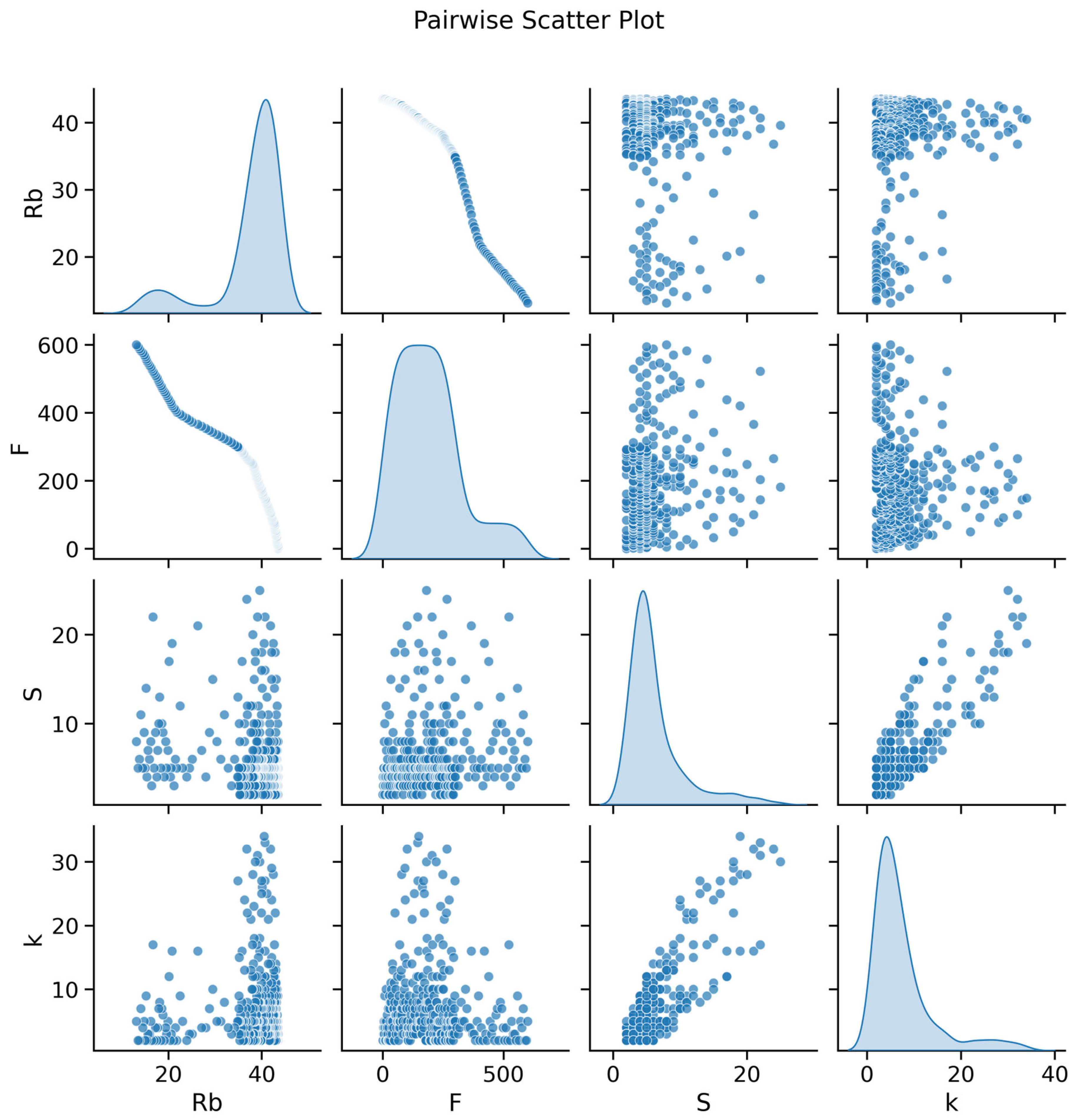
Figure 3 shows a plot created using the Pairplot method from the Seaborn library [55]. The X and Y axes of each diagram represent the values of two different variables, allowing for a visual assessment of the relationships between all pairs of features. The main diagonal is constructed differently. The main diagonal (where the variable intersects with itself) displays univariate distributions, showing the marginal distribution of the data in each column.

Figure 3. Scatterplots.

Figure 3 presents the scatterplots. The visualizations of the numerical data located on the main diagonal allow for an analysis of data bias. For the strength column, the data are skewed toward the range of 35 to 45 MPa, for the “Average Damage Area” column, the greatest number of data points are observed in the range of 2 to 7 mm², and the most frequently occurring value for the number of detected damaged areas is distributed between 2 and 7. When analyzing the scatterplot, it is worth noting that no obvious clusters were detected. A linear relationship is observed between R_b and F. Another valuable insight is the upward trend from left to right for the S and k columns, indicating a positive correlation (which is true, as the average area increases with increasing damage count).

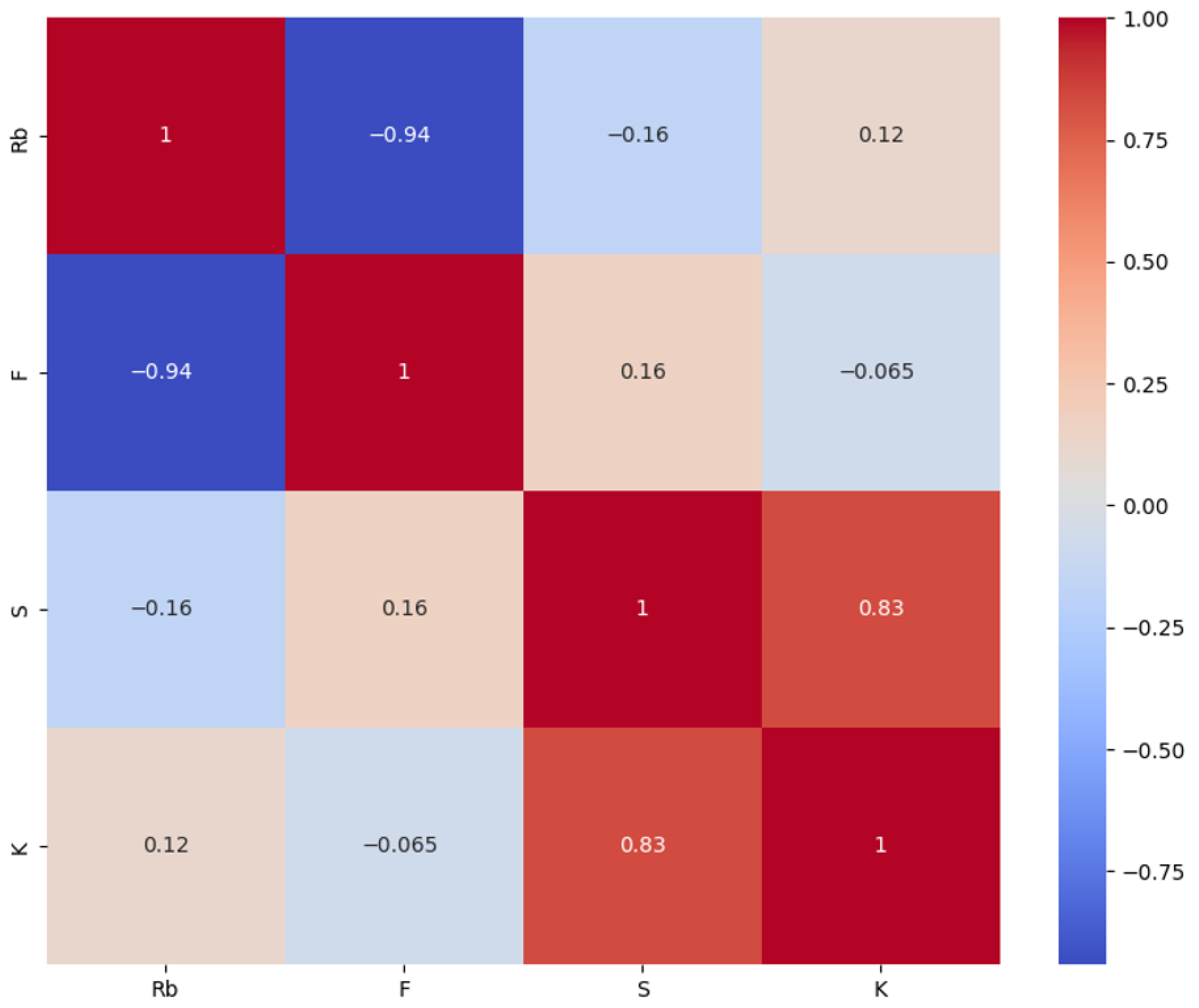
Figure 4 shows a correlation matrix that allows us to accurately determine the strength of the relationship between columns in the dataset. The target column R_b is most strongly influenced by the number of freezes (F), with a strength of 0.94.

Figure 4. Correlation Matrix.

2.4. Selection and Creation of AI Models

In this study, the following models are proposed for implementation:

• Linear Regression, a parametric linear method.
• K-Neighbors (KNN), a metric method.
• Decision Tree, a tree-structured method.
• Random Forest, a tree-structured method.
• CatBoost, a tree-structured method.
• Support Vector Regression (SVR), a nonparametric kernel-based method.
• Multilayer Perceptron (MLP), an artificial neural network.

These machine learning models are based on various underlying approaches for modeling complex linear and nonlinear dependence that exists between input features and the target variable. Various solutions will facilitate identifying the most effective method for forecasting concrete and component strength in harsh environments.

Finding optimal values for the model’s key parameters is a key step in achieving the best generalization. This research employed a grid search with three-box cross-validation to examine all potential parameter combinations for each model. The parameter grid was formed taking into account the small size of the dataset. For example, for the k-nearest neighbors method, this imposes limitations on the choice of the number of neighbors. A large value for this parameter may prevent the model from capturing subtle patterns in the data. For tree-based methods, a small dataset size influences the choice of tree depth (they should not be too deep), as well as the minimum number of samples required to split an internal node of each tree. In this study, the search for the best parameters was carried out on a fixed grid of possible values. In further development of the study, it is planned to apply bisection search and fine-tuning (FT), which will improve the forecasting quality [56]. During the implementation of the algorithm, reproducibility of results across all model series was ensured, ensuring identical fold partitions. This approach enables subsequent comparison of models using key metrics.

The model’s execution process, which incorporates cross-validation and a parameter grid, is presented in Figure 5. The training and test sets were split 80/20.

Figure 5. Model evaluation and parameter selection utilizing a parameter grid and three-way cross-validation.

2.4.1. Linear Regression

Linear regression was the first technique utilized in this investigation. This is a fundamental and extensively utilized technique for resolving regression problems.

In the context of solving a regression problem, it is essential to arrange the actual response Y from the input vector $X^{\mathrm{T}}=\left(X_1,X_2,\dots ,X_p\right)$.

The linear regression model has the following form:

$$f\left(X\right)={\beta }_0+{\displaystyle \sum _{j=1}^p{X}_j{\beta }_j}$$

(2)

where ${\beta }_j$ are the model coefficients (weights); and ${\beta }_0$ is the bias.

To determine the regression model’s weights and bias, the loss function must be minimized.

$$L_{MSE}={\displaystyle \frac{1}{N}}{\displaystyle \sum _{i=1}^N{\left(y_i-f\left(x_i\right)\right)}^2}$$

(3)

As a result of fitting the linear model, the following equation was obtained:

$$y=37.6482-6.3775F-1.4837S+1.6092k$$

(4)

2.4.2. K-Neighbors

Regression problems are solved using the supervised machine learning algorithm known as k-nearest neighbors (KNN). Its efficacy is notable when handling small datasets, an attribute of considerable significance for our purposes.

In practical applications, the KNN method is more frequently employed for classification tasks, although the regression version of the k-neighbors algorithm is also extensively utilized. This constitutes a solid, preliminary algorithm, appropriate for initial experimentation before the implementation of more complex methodologies.

The algorithm determines the distances between a query and every example in the data, selects the k-nearest neighbors to the query, and then computes the average of the labels for regression problems.

To obtain accurate strength prediction results when implementing the k-neighbors method, it is necessary to determine the optimal value of the n_neighbors parameter. If the value is too small, overfitting occurs. If the value for this parameter is too large, too many objects from different freezing cycles will be included in the prediction. Such a forecast may yield overly coarse values and poorly reflect local characteristics during the transition from one freezing cycle to the next. Therefore, the choice of the n_neighbors parameter is a compromise between accuracy and the generalizability of the model.

The parameter in this research was chosen from the following variations: n_neighbors: [3,5,7]. The optimal value during cross-validation was n_neighbors = 3.

2.4.3. Decision Tree

A nonparametric supervised learning method called decision trees is used to solve regression problems. The DT decision tree architecture estimates the value of a dependent variable using straightforward decision rules extracted from data features [57]. Trees can be considered piecewise constant approximations. Commercial and industrial data mining applications have a high demand for this predictive analysis method [58].

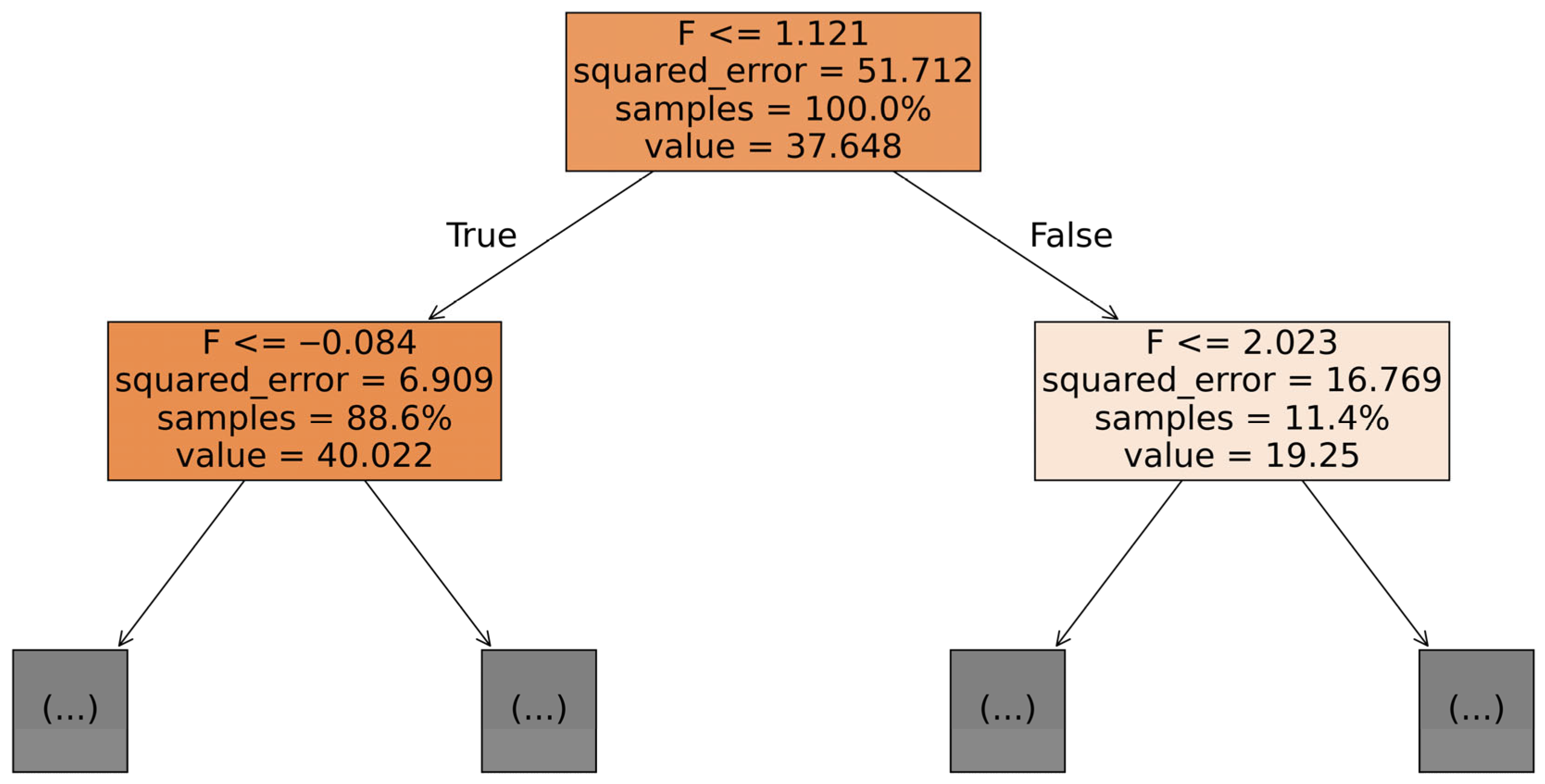
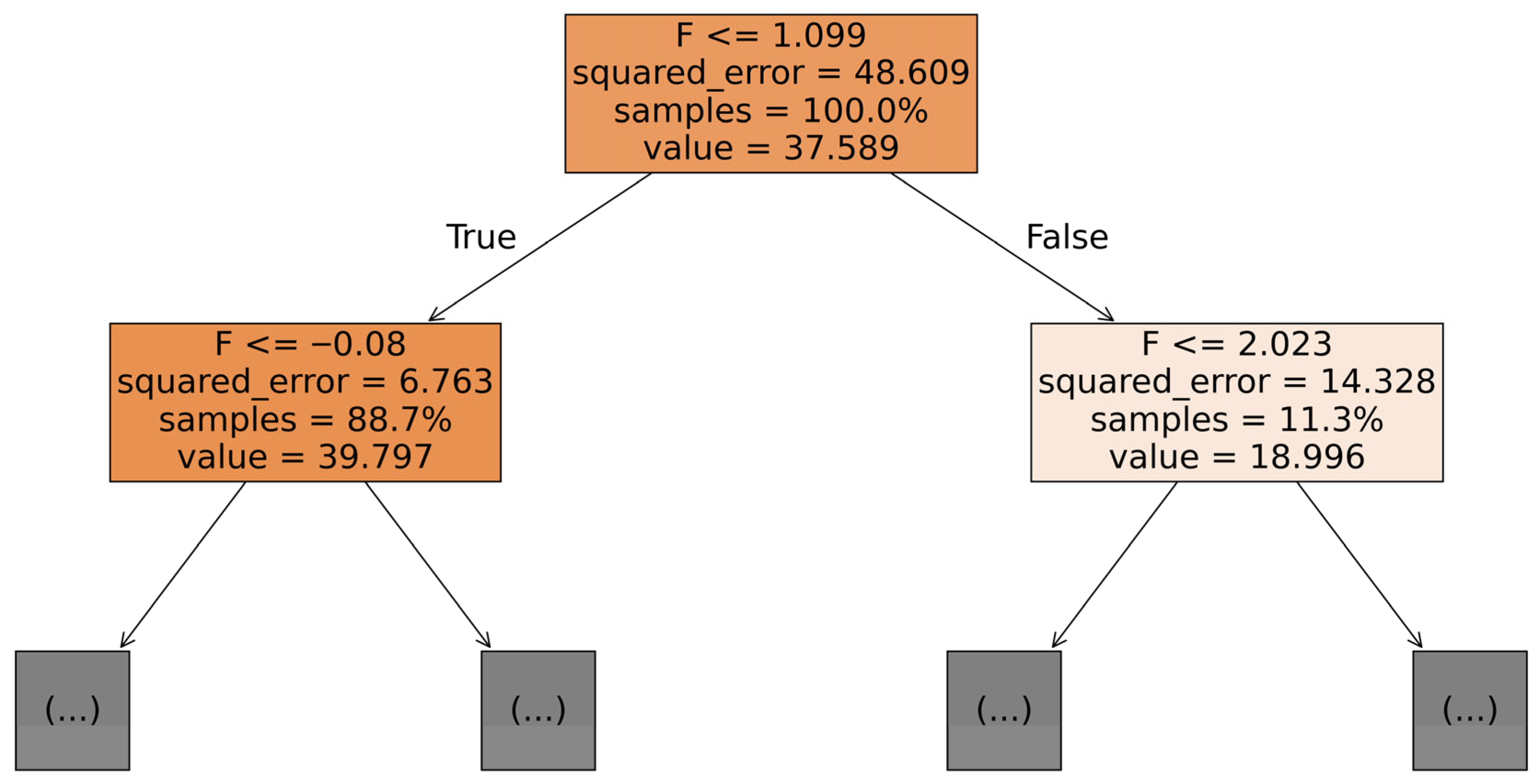
One of the primary advantages of Decision Tree method is its understandability and logical interpretation. A researcher can visualize trees. Figure 6 presents a visual representation of the tree developed for this research. A drawback is that the algorithm may create overly complex, overfitted trees during execution. Hyperparameter optimization is essential to reduce overfitting in a tree susceptible to this issue.

Figure 6. Decision Tree.

During the selection of optimal parameters, the following were varied:

“maximum tree depth” ‘max_depth’: [3,5,7] and “minimum number of samples required to split an internal node of each tree” ‘min_samples_split’: [2,5,10]. The following combination demonstrated the best prediction quality: {‘max_depth’: 7, ‘min_samples_split’: 2}.

2.4.4. Random Forest

A decision tree combination makes up a predictive model, which is known as a regression tree ensemble. Each of these trees, on its own, produces a low-quality regression, but their large number produces a satisfactory result. Therefore, integrating regression trees improves predictive capabilities.

The research employed an ensemble regression tree model, and it adjusted various parameters to identify the most optimal configurations.

Predictive accuracy in an ensemble typically depends on the use of several hundred to several thousand “weak learners”. For small samples, it is best to start with a several trees, then evaluate the ensemble’s effectiveness, and increase their number if necessary. In this study, the number of trees spanned four ‘n_estimators’ values: [20,50,100,200]. Figure 7 shows one of the decision trees.

Figure 7. Random Forest Decision Tree.

Another important hyperparameter to tune is the depth of the decision trees. The study evaluated the depth effectiveness for the following ‘max_depth’ values: [3,5,7].

The best combination for Random Forest is: {‘n_estimators’: 100,’ max_depth’: 7}.

The trees are deep, but achieving good results did not require increasing their number to the maximum suggested by the parameter grid (up to 200).

2.4.5. CatBoost

CatBoost is a machine-learning technique created by Yandex (Moscow, Russia) for gradient boosting using decision trees. Compared to ordinary layer-by-layer tree construction, this methodology, which utilizes symmetric trees, offers substantial performance advantages in most instances.

This approach was selected for this study because of its ability to provide good results with a relatively small dataset, unlike other machine learning algorithms, which require a large training set to perform effectively. Model parameters require adjustment to mitigate overfitting. As with the two previous tree structures, the tree depth ‘depth’ was adjusted to [3,5,7] and the “learning rate” ‘learning_rate’ to [0.01, 0.1]. The best combination for CatBoost was {‘depth’: 3, ‘learning_rate’: 0.1}.

It should be noted that the tree depth was reduced to 3, while the learning rate was set to the highest possible value.

2.4.6. Support Vector Regression

Support Vector Regression (SVR) represents an evolution of Support Vector Machines (SVM), tailored for regression applications. Support Vector Regression necessitates labeled training data within the supervised learning framework. In this case, the “R_b, MPa” response column allows us to train the model in a supervised manner. SVR incorporates an additional, user-defined parameter, epsilon (ε). The epsilon parameter defines the margin around the estimated function (hyperplane). Correct predictions are considered to be those points that fall within this “tube.” The support vectors consist of those data points that are positioned outside the tube. The magnitude of the slack variable (ξ) provides a measure of the extent of separation from the tube, which is controllable by altering the regularization parameter C.

However, the basic idea is always the same: minimize error by customizing the hyperplane.

In this study, the following parameters were used to construct the SVR model: {‘C’: 10, ‘kernel’: ‘rbf’}. The quadratic exponential kernel ‘rbf’ is highly flexible and adaptable and is preferred for most regression problems.

2.4.7. Multilayer Perceptron

A multilayer perceptron (MLP) is a supervised learning algorithm. Given a set of features $X=\left\{x_1,x_2,\dots ,x_m\right\}$ and a target variable y, a nonlinear function approximator is trained to solve a regression problem. In our case:

$x_1$ is the number of freezing cycles;

$x_2$ is the average area of damaged areas;

$x_3$ is the number of detected areas;

y is the compressive strength.

The architecture of the selected artificial neural network (ANN) consists of an input layer, one hidden layer, and an output layer of interconnected neurons. The number of neurons in the inner layer was selected from the following options: ‘hidden_layer_sizes’: [(50,), (100,)], and the activation function was represented by the set ‘activation’: [‘relu’, ‘tanh’]. The MSE is used as the loss function. The MLP is trained using stochastic gradient descent. The best parameter combinations during optimization were the following: {‘activation’: ‘tanh’, ‘hidden_layer_sizes’: (100,)}.

2.5. Evaluation of Quality Metrics

To evaluate the accuracy of trained models and select a machine learning algorithm for further recommendations, quality metrics should be used. In this study, the following metrics were evaluated.

MAE (Mean Absolute Error) is a metric that measures the average size of forecast errors, regardless of their direction. It is calculated as the arithmetic mean of the absolute differences between the actual (real) and predicted values.

$$MAE={\displaystyle \frac{1}{n}}{\displaystyle \sum _{i=1}^n\left|y_i-{\widehat{y}}_i\right|}$$

(5)

MSE (Mean Squared Error) is a metric in machine learning that evaluates the quality of regression models by measuring the average of the squared differences between actual and predicted values.

$$MSE={\displaystyle \frac{1}{n}}{\displaystyle \sum _{i=1}^n{(y_i-{\widehat{y}}_i)}^2}$$

(6)

RMSE (Root Mean Squared Error) is a metric in machine learning used to evaluate the accuracy of regression models, measuring the average deviation of actual values from predicted ones by squaring the difference, averaging these squares, and extracting the square root.

$$RMSE=\sqrt{{\displaystyle \frac{1}{n}}{\displaystyle \sum _{i=1}^n{(y_i-{\widehat{y}}_i)}^2}}$$

(7)

MAPE is a Mean Absolute Percentage Error metric used to evaluate the accuracy of forecasts by measuring the average percentage deviation of the forecast from the actual value.

$$MAPE={\displaystyle \frac{1}{n}}{\displaystyle \sum _{i=1}^n\left|\frac{y_i-{\widehat{y}}_i}{{\widehat{y}}_i}\right|}\times 100$$

(8)

The R² metric, or coefficient of determination, is a measure of the variability in the dependent variable that can be explained by the independent variables in a regression model.

$$R^2=1-{\displaystyle \frac{{\displaystyle \sum _{i=1}^n{\left(y_i-{\widehat{y}}_i\right)}^2}}{{\displaystyle \sum _{i=1}^n{\left(y_i-\overline{y}\right)}^2}}}$$

(9)

3. Results and Discussion

The development of machine learning-based algorithms was executed using the high-level Python 3.14.0 programming language within the Jupyter Notebook Version: 5.9.1 interactive web computing platform for this study. The underlying libraries used for the study were Pandas 2.2.2, Numpy 2.0.2, Seaborn 0.13.2, Matplotlib 3.9.0, and Sklearn 1.6.1.

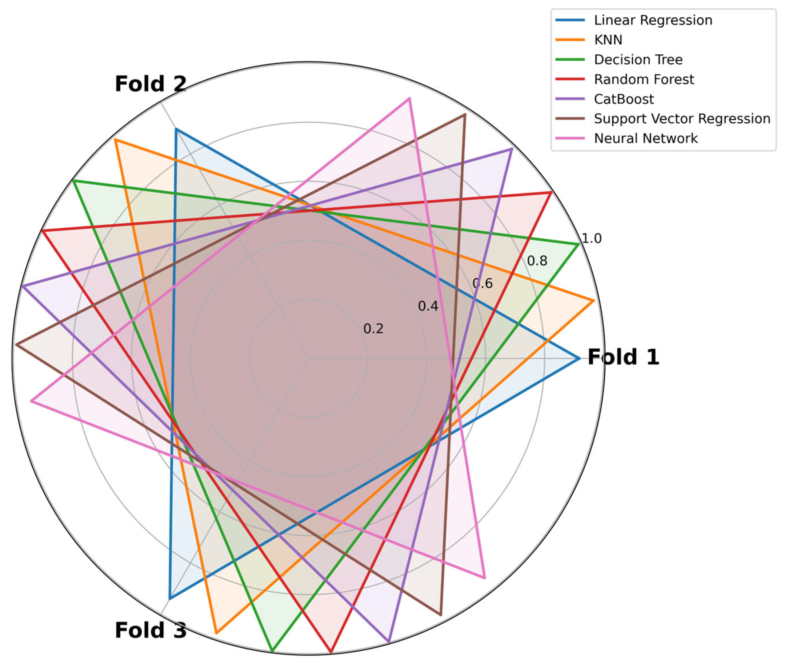
Figure 8 shows the coefficient of determination values of the models for each fold, indicating that the model performs well in different parts of the data.

Figure 8. R² by folds.

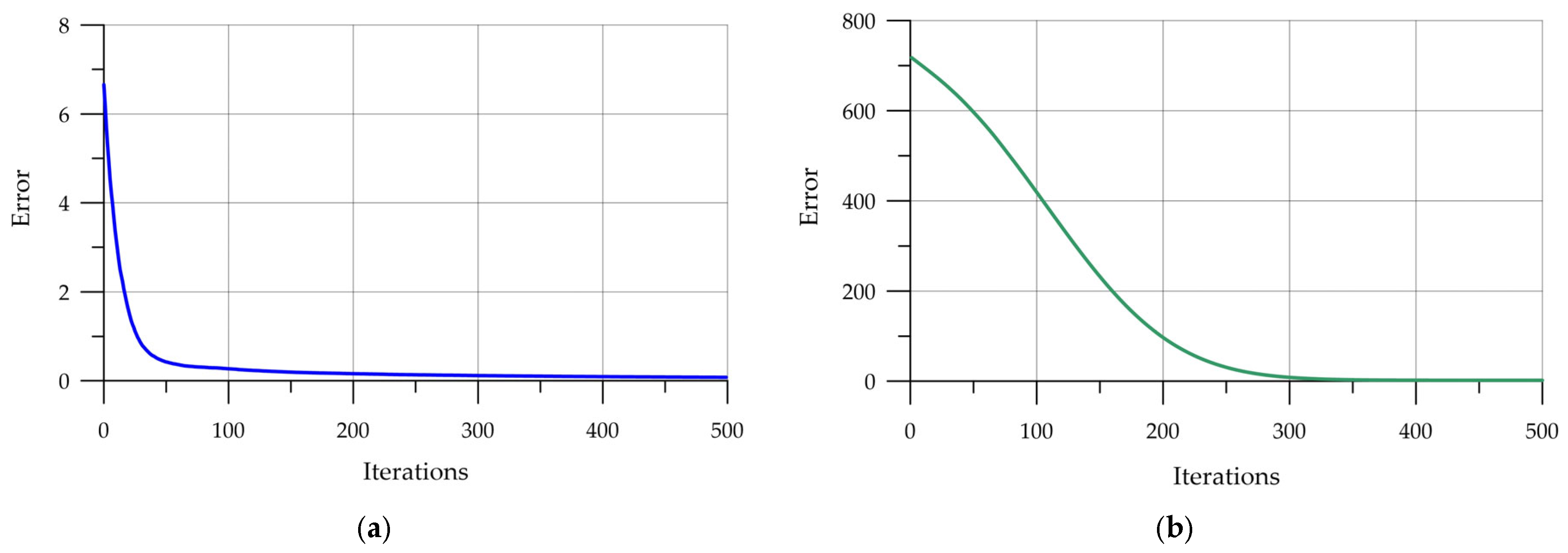
For the CatBoost (CB) and Multilayer Perceptron (MLP) models, the training process can be visualized. Analysis of the CB training graph (Figure 9a) shows that training is stable, with the RMSE metric chosen as the loss function steadily decreasing. No overfitting is observed in the graph. To monitor for overfitting, an early stopping method was used, which terminates training if no significant drop in error is observed within 10 iterations. MLP training also proceeds stably, with the MSE error significantly decreasing after 200 iterations (Figure 9b).

Figure 9. Training: (a) CB (b) MLP.

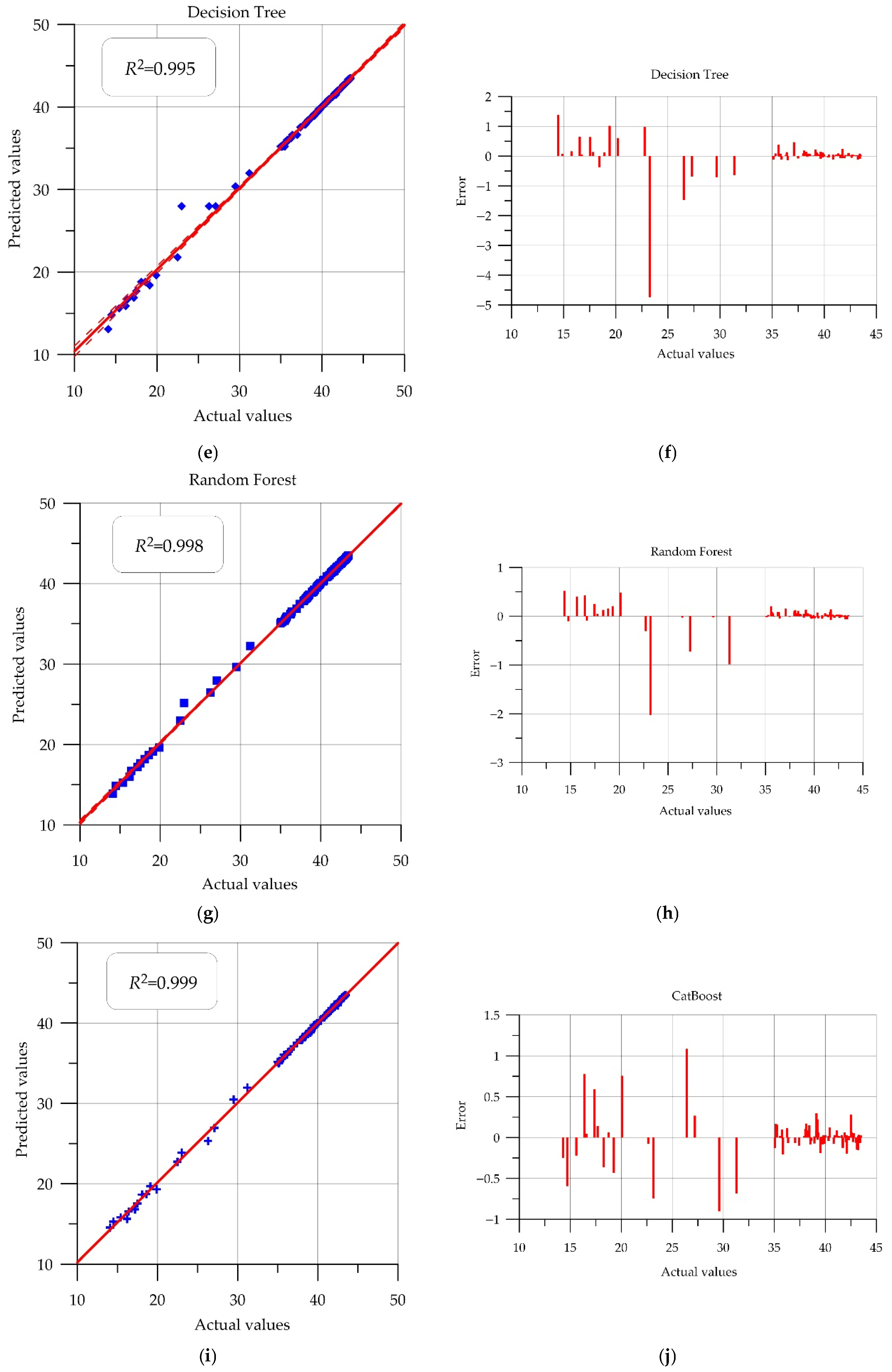
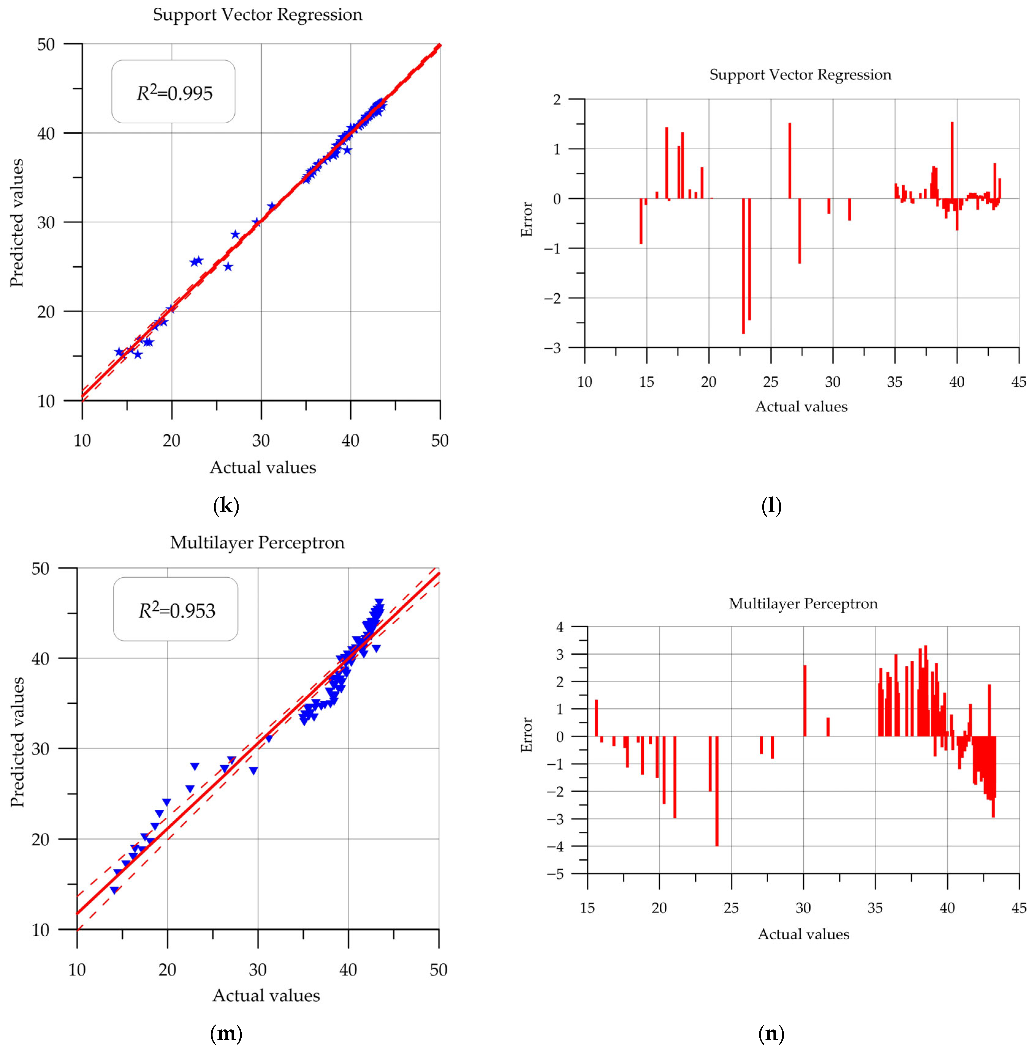
To evaluate the forecasting quality, a visual component was used—a scatterplot of predicted and actual values (Figure 10). In this plot, the x-axis represents the actual strength values from the test sample, and the y-axis represents the values predicted by the model. A line drawn from the center at a 45° angle allows for a visual assessment of the distribution of points: the closer they are to the line, the more accurate the forecast. If the points were above the line, the network predicted higher strength than the actual values, and if the points were below the line, the predicted values were lower than the actual values.

Figure 10. Actual vs. Predicted and error residuals: (a,b) Linear Regression; (c,d) K-Neighbors; (e,f) Decision Tree; (g,h) Random Forest; (i,j) CatBoost; (k,l) Support Vector Regression; (m,n) Multilayer Perceptron.

For the linear regression model in Figure 10a, we see that the model predicts higher values in the strength ranges of 15–25 MPa and 42–45 MPa, while the opposite is true for the 35–42 MPa range.

When analyzing the scatterplot for the k-nearest neighbors method, it is worth noting the improved location of the points relative to the drawn control line, indicating improved prediction quality.

When analyzing the decision tree plot, it is worth noting that this tree structure most accurately predicts strengths above 35 MPa.

The results for the random forest tree structure demonstrate good accuracy across the entire range of strengths considered. The points are clustered close to the straight line, indicating high model quality. The results of the CatBoost model are comparable to those of the decision tree: an improvement in prediction is also observed from 35 MPa.

The support vector regression method, based on constructing a hyperplane that optimally separates the sample objects, is successful in predicting concrete strength, with no obvious outliers observed.

When examining the prediction results for the multilayer perceptron, it is worth noting the relatively large scatter of points around the control line. This distribution yields the lowest prediction quality compared to previous models.

Table 2 presents the final quality metrics for the test set obtained by the machine learning models under consideration.

Table 2. Final Quality Metrics.

Num	Model	MAE	MSE	RMSE	MAPE, %	R2
1	LR	1.95	5.31	2.31	6.55	0.92
2	KNN	0.42	0.43	0.65	1.38	0.99
3	DT	0.19	0.32	0.57	0.8	0.99
4	RF	0.09	0.07	0.27	0.4	1.00
5	CB	0.14	0.06	0.25	0.5	1.00
6	SVR	0.29	0.31	0.55	1.09	1.00
7	MLP	1.46	2.99	1.73	4.59	0.95

It is worth noting that when solving this problem, the priority metrics to consider when selecting the best method are RMSE, MAPE, and R².

The RMSE error value is shown in the same physical units as the forecast column, that is, in MPa. The RF and CB methods demonstrate the smallest errors: deviations from the actual values are 0.27 MPa and 0.25 MPa, respectively. A similar result is observed when analyzing the MAPE column: the RF and CB methods demonstrate an error of less than 1%. These machine learning algorithms are less sensitive to dataset size when properly configured, while still being able to capture nonlinearities in the data. They are ensemble-based and tree-based, a structure that makes them robust to noise. Their basic architecture, which also incorporates internal principles of regularization and randomness in feature selection, enables them to demonstrate good forecasting results.

The R² coefficient of determination for both models is above 0.99. High values for this statistical measure indicate that the implemented models describe changes in the observed data well.

The linear regression and artificial neural network models performed poorly in terms of forecasting. It is believed that linear regression demonstrated low accuracy due to its simplicity. The ANN model showed good results during training, but an error of 4.59% was obtained on the test set. It is believed that fine-tuning of the hyperparameters would allow the neural network to better adapt to identifying hidden dependencies in the data.

Comparing the obtained results with models already available in the scientific field, it is worth noting that good quality metrics were achieved in the present study. In the study [47], the coefficient of determination for the best hybrid models was 0.95–0.97. In the present study, the R² metric also starts at 0.95 and reaches 1.00. In [48], the SVR algorithm demonstrates high accuracy and predictive power with an R² value of 0.95 and an RMSE of 3.40 MPa. This method also demonstrated positive results in the present study, achieving an R² value of 1.00 and an RMSE of 0.55 MPa. The decision tree gradient boosting algorithm in [49] demonstrated the following forecast errors: MAE 0.1351 MPa, RMSE 0.1842 MPa, and MAPE 0.48%. The CB gradient boosting algorithm in the present work demonstrated comparable results: MAE 0.14 MPa, RMSE 0.25 MPa, and MAPE 0.5%.

The proposed model for predicting the properties of heavy-duty concrete, using machine learning methods, will reduce the development time for new concretes by eliminating the need for laboratory experiments. The model enables targeted searches for new building materials with specified characteristics. Subsequently, test samples must be produced and their properties confirmed through testing.

Implementation of this approach will allow the construction industry to respond more flexibly and quickly to new challenges. For example, it will enable the rapid development of heavy-duty concrete with specified characteristics for the design and construction of unique buildings and structures. Concretes developed using machine learning methods will have superior properties compared to materials obtained using traditional approaches, as machine learning methods enable the solution of multifactorial problems and evaluate a combination of factors during the life of the building material.

Economically, the reduction in labor costs and human resources needed to create a building material results in lower production expenses, enhancing the manufacturer’s competitive standing in the construction sector. For the population, the introduction of heavy-duty concrete produced using machine learning methods will lead to lower housing prices and make housing more affordable.

Compared to classical mathematical modeling, improving a machine learning algorithm is significantly simpler than refining a mathematical model when studying physical processes, which is especially important with the rapid introduction of new building materials with fundamentally different properties.

The findings from implementing seven machine learning methods with diverse underlying frameworks confirm the general trend in domestic and international practice toward using a variety of machine learning methods to predict the strength properties of concrete.

It is important to highlight the practical recommendations for using the developed algorithms. All models are adaptive and scalable, and can be deployed locally or as part of an online system. There is a widespread trend toward integrating AI systems into real-world projects. For example, the Canadian government is investing in Giatec Scientific Inc. and its AI-driven concrete demonstration plant [59]. This will enable the use of sensor and software technologies to monitor concrete throughout its entire lifecycle.

The intelligent methods proposed in this study have several limitations. First, it is worth noting that this specific example only examined the effects of freeze–thaw cycles, but in reality, many other factors can influence a material. Therefore, when adapting these methods to specific conditions, it is necessary to conduct a thorough analysis of the subject area and identify all significant quantitative and qualitative factors that can positively or negatively influence strength properties.

It is worth noting a number of computational limitations associated with the implementation of intelligent models in real-world production. At an industrial scale, high speed is required to generate forecasts. This study involves processing data using CV and then running the forecast model. With large data volumes, this can introduce delays. However, using GPU-equipped servers and parallel processing methods will minimize the time it takes to receive results.

4. Conclusions

This paper implements machine learning methods (Linear Regression, K-Neighbors, Decision Tree, Random Forest, CatBoost, Support Vector Regression, and Multilayer Perceptron) to predict the properties of heavy concrete, specifically compressive strength. Parameter selection and model evaluation were performed using a parameter grid and three-part cross-validation. After laboratory studies and testing, a database was compiled containing 351 rows and the following input parameters: F, freeze–thaw cycle; S, average area of damaged areas; k, number of damaged areas; Rb, specimen strength. The performance of the developed models was evaluated using various quality metrics, such as MAE, MSE, RMSE, MAPE, and R².

The tree-based Random Forest and CatBoost methods demonstrated the lowest errors: deviations from actual values were 0.27 MPa and 0.25 MPa, respectively, with an average absolute percentage error of less than 1%. The R² determination coefficient for both models is greater than 0.99.

The results of the study represent a contribution to the study of the behavior of heavy concrete under aggressive environmental conditions.

The following actions can be taken to improve the model:

-

expanding the training set through additional laboratory tests;

-

expanding the training set from open sources;

-

accounting for the impact of other types of aggressive environmental influences (e.g., wetting and drying);

-

developing other ML methods for solving predictive problems;

-

adapting the proposed methods to other types of concrete, taking into account the specifics of their formulation.

Furthermore, this machine learning model can be improved by expanding the number of predicted parameters for the building material being developed. For example, it is possible to include characteristics such as thermal conductivity, durability, porosity, vapor permeability, or static moisture conductivity of the material in the analysis to obtain a sample with the desired properties. The implementation of hybrid systems like ensemble ML model is planned for further research after expanding the dataset with other features.